Variational equivalence between Ginzburg-Landau, XY spin systems and screw dislocations energies

Roberto Alicandro Marco Cicalese  and  Marcello Ponsiglione DAEIMI, Università di Cassino via Di Biasio 43, 03043 Cassino (FR), Italy alicandr@unicas.it Dipartimento di Matematica e Applicazioni “R. Caccioppoli”, Università di Napoli “Federico II” via Cintia, 80126 Napoli, Italy cicalese@unina.it Dipartimento di Matematica “G. Castelnuovo”, Universitá di Roma “La Sapienza”, Piazzale A. Moro 2, 00185 Roma, Italy ponsigli@mat.uniroma1.it Roberto Alicandro
DAEIMI, Università di Cassino
via Di Biasio 43, 03043 Cassino (FR), Italy
e-mail: alicandr@unicas.it Marco Cicalese
Dipartimento di Matematica e Applicazioni “R. Caccioppoli”
Università di Napoli “Federico II”
via Cintia, 80126 Napoli, Italy
e-mail: cicalese@unina.it Marcello Ponsiglione
Dipartimento di Matematica “G. Castelnuovo”
Universitá di Roma “La Sapienza”
Piazzale A. Moro 2, 00185 Roma, Italy
e-mail: ponsigli@mat.uniroma1.it
Abstract.

We introduce and discuss discrete two-dimensional models for $XY$ spin systems and screw dislocations in crystals. We prove that, as the lattice spacing $\varepsilon$ tends to zero, the relevant energies in these models behave like a free energy in the complex Ginzburg-Landau theory of superconductivity, justifying in a rigorous mathematical language the analogies between screw dislocations in crystals and vortices in superconductors. To this purpose, we introduce a notion of asymptotic variational equivalence between families of functionals in the framework of $\Gamma$-convergence. We then prove that, in several scaling regimes, the complex Ginzburg-Landau, the $XY$ spin system and the screw dislocation energy functionals are variationally equivalent. Exploiting such an equivalence between dislocations and vortices, we can show new results concerning the asymptotic behavior of screw dislocations in the $|\log\varepsilon|^{2}$ energetic regime.

Keywords: Crystals, Discrete-to-continuum limits, Analysis of microstructure, Topological singularities, Calculus of Variations. 2000 Mathematics Subject Classification: 49J45, 74N05, 74N15, 74G70, 74G65, 74C15, 74B15, 74B10.

1. Introduction

Since the pioneering papers of Berezinskii [6], Kosterlitz [25] and Kosterlitz and Thouless [26], there has been a great effort in studying physical systems exploiting BKT-phase transitions; i.e., phase transitions mediated by the formation of topological singularities of the order parameter. This type of phase transitions characterizes several physical phenomena such as superfluidity, superconductivity and plasticity (see [24], [27], [28], [29], [34]), while vortices in superconductivity and $XY$ spin systems, as well as screw dislocations in crystals, provide three paradigmatic examples of singularities.

The phenomenological analogies shown by these apparently far physical systems have been pointed out many times in the physical community. In the language of statistical mechanics it has also been rigorously proven that these systems belong to the same universality class all of them sharing a BKT-type phase transition. Roughly speaking it is known that above some temperature threshold, these systems undergo a phase transition to a disordered state in which the topological singularities are unbound. Under that threshold the correlation length exponentially decays and the singularities bind together and interact through complex and mostly unknown phenomena involving many interacting scales. Such a complex behavior is the main reason why a detailed analysis of the ground states of these systems turns out to be a non trivial task. Moreover, the above description explains, to some extent, why a qualitative approach to the study of the thermodynamic limit of these systems, such as the celebrated Ginzburg-Landau theory, has been so successfully exploited.

In this paper we are concerned with the problem of describing some relevant properties of the ground states of these systems in the thermodynamic limit. We aim to provide a unifying mathematical point of view, based on a variational equivalence argument, to study the asymptotic behavior of the ground states of different models that share the same geometrical and topological qualitative features. More specifically our purpose is two-fold. On one hand, we want to reinterpret several known results about the asymptotic behavior of the ground states of such models, proving that the corresponding free energies are indeed equivalent from a variational point of view. On the other hand, taking advantage of this equivalence, we want to exploit some of the results currently proved only through a phenomenological Ginzburg-Landau analysis, to obtain new results in different contexts.

As in [26], among the physical systems exploiting topological type phase transitions we focus on two-dimensional systems and we choose two paradigmatic examples: screw dislocations ($SD$) and $XY$ spin systems. We will introduce two basic discrete models, both constructed on $\varepsilon{\mathbb{Z}}^{2}\cap\Omega$, where $\Omega\subset{\mathbb{R}}^{2}$ is a bounded open set. Their order parameters are a unit vectorial spin field for the $XY$ model: $i\in\varepsilon{\mathbb{Z}}^{2}\cap\Omega\mapsto v(i)\in{\mathbb{R}}^{2}$ such that $|v(i)|=1$, and a scalar displacement field for the $SD$ model: $i\in\varepsilon{\mathbb{Z}}^{2}\cap\Omega\mapsto u(i)\in{\mathbb{R}}$. For a given configuration of spins or displacements, the energies of these systems are given by

$$XY_{\varepsilon}(v):=\frac{1}{2}\sum_{i,j\in\varepsilon{\mathbb{Z}}^{2}\cap\,\Omega:\ |i-j|=\varepsilon}|{v(i)-v(j)}|^{2}$$

and

$$SD_{\varepsilon}(u):=\frac{1}{2}\sum_{i,j\in\varepsilon{\mathbb{Z}}^{2}\cap\,\Omega:\ |i-j|=\varepsilon}\text{dist}^{2}(u(i)-u(j),{\mathbb{Z}}).$$

With the energies written in this form, the coarse-graining analysis now amounts to study the limit, as $\varepsilon\to 0$, of (some scaled version of) $XY_{\varepsilon}$ and $SD_{\varepsilon}$. To this purpose, in the physical literature, it is customary to perform a so-called Ginzburg-Landau (GL) analysis (see [24] and [34] for an introduction to the subject and some applications). The main ansatz of this approach (based on heuristic scaling and symmetry type arguments) is to assume that some of the interesting features of the thermodynamic limit of the original functionals can be obtained by studying the limit, as $\varepsilon\to 0$, of a family of so-called complex Ginzburg-Landau energies. These energies have as order parameter a vectorial field $x\in\Omega\mapsto w(x)\in{\mathbb{R}}^{2}$ and are defined as

(1) $$GL_{\varepsilon}(w):=\int_{\Omega}\frac{1}{2}|\nabla w|^{2}+\frac{1}{\varepsilon^{2}}(1-|w|^{2})^{2}.$$

This kind of functionals has been originally introduced as a phenomenological phase-field type free-energy of a superconductor, near the superconducting transition, in absence of an external magnetic field. Here the order parameter $w$ describes how deep the system is into the superconducting phase and the scale $\varepsilon$ is proportional to the coherence length of the superconductor.

The Ginzburg-Landau functionals have deserved a great attention by the physical community. The first rigorous mathematical approach to the limit as $\varepsilon\to 0$ of the solutions to the Euler-Lagrange equation of (1) has been made by Bethuel, Brezis and Hélein in [7]. Since their paper a great effort has been done to study the asymptotic behaviour of minimizers of the Ginzburg-Landau energy both from the PDEs and the Calculus of Variations points of view. In particular in dimension two Jerrard and Soner in [22] (see also Alberti, Baldo and Orlandi [1] for the generalization to any dimension) have proved a $\Gamma$-convergence result for $\frac{GL_{\varepsilon}(w)}{|\log\varepsilon|}$. In their analysis the relevant tool to track energy concentration is the asymptotic behavior of the Jacobians $J(w_{\varepsilon})$ of sequences $(w_{\varepsilon})$ equi-bounded in energy. In particular they prove that, up to subsequences, $J(w_{\varepsilon})$ converges to a finite sum of Dirac deltas whose support represents the vortex-like singularities of the limit field and that the $\Gamma$-limit is proportional to the number of such singularities.

Only recently a similar analysis in the context of spin systems and dislocations has attracted much attention in the mathematical community and it has been carried on both in a continuous framework (see [13], [14], [19], [20]) and in a discrete setting (see [2], [3], [4], [30]). As a further remark we underline that the asymptotic analysis of spin systems and discrete dislocations energy functionals is itself part of a wider interest in the discrete-to-continuum limits for more general models (see for example [8], [9] and [11] (Chapter $11$) for a review on this subject).

In [3] and in [30] a $\Gamma$-convergence result for $XY$-spin systems and for the $SD$ model is given in the $|\log\varepsilon|$ scaling regime. Here the $\Gamma$-convergence analysis is performed with respect to the convergence of the Jacobians of a suitable affine interpolation of the spin variable $v$ for the $XY$ model, and with respect to the convergence of a suitable discrete notion of the ${\it curl}$ of the strain field $u$ for the $SD$ model. Roughly speaking, gathering together the main results of these two papers, the following relations hold:

$$\Gamma\hbox{-}\lim_{\varepsilon\to 0}\frac{GL_{\varepsilon}(w)}{|\log\varepsilon|}=\Gamma\hbox{-}\lim_{\varepsilon\to 0}\frac{XY_{\varepsilon}(v)}{|\log\varepsilon|}=\Gamma\hbox{-}\lim_{\varepsilon\to 0}\frac{4\pi^{2}SD_{\varepsilon}(u)}{|\log\varepsilon|}.$$

Motivated by this chain of equalities, we were led to ask whether one could provide, in the framework of $\Gamma$-convergence, a unifying mathematical point of view to rigorously relate the asymptotic behavior of these models. Our purpose is to prove that the asymptotic equivalence of these models, in terms of $\Gamma$-convergence, can be push forward to any $|\log\varepsilon|^{h}$ scaling regime with $h\geq 1$. More precisely, we show that

(2) $$\Gamma\hbox{-}\lim_{\varepsilon\to 0}\frac{GL_{\varepsilon}(w)}{|\log\varepsilon|^{h}}=\Gamma\hbox{-}\lim_{\varepsilon\to 0}\frac{XY_{\varepsilon}(v)}{|\log\varepsilon|^{h}}=\Gamma\hbox{-}\lim_{\varepsilon\to 0}\frac{4\pi^{2}SD_{\varepsilon}(u)}{|\log\varepsilon|^{h}}.$$

In this way we rigorously obtain the equivalence of some mean field models for vortices, spin systems and dislocations, according with experimental evidence (see [31] for a recent overview of the analogies between the mean fields in these models). In particular, we obtain a rigorous justification to the $GL$ analysis of the thermodynamic limits of the $XY$ and $SD$ models in the $|\log\varepsilon|^{h}$ energetic regimes.

To prove (2), we look for a relation between the order parameters of the different models, at proper mesoscopic scales, which allow us to compare the three families of energy functionals in the $|\log\varepsilon|^{h}$ scaling regime for every $h\geq 1$. This has led us to introduce a notion of variational equivalence between families of functionals (see Definition 7). To explain the meaning of such a notion, let us suppose that we are given two families of energies $(F_{\varepsilon})$ and $(G_{\varepsilon})$ depending on a small parameter $\varepsilon$ standing for an interaction scale. Then we say that $(F_{\varepsilon})$ and $(G_{\varepsilon})$ are variationally equivalent if there holds that $G_{\varepsilon}\preceq F_{\varepsilon}$ and $F_{\varepsilon}\preceq G_{\varepsilon}$. By $G_{\varepsilon}\preceq F_{\varepsilon}$ we mean that, for any given family of order parameters $(p_{\varepsilon})$ such that $F_{\varepsilon}(p_{\varepsilon})\leq C$, there exists another scale $\delta_{\varepsilon}$ and a family of order parameters $q_{\varepsilon}$ such that $q_{\varepsilon}$ is closer and closer to $p_{\varepsilon}$ and $G_{\delta_{\varepsilon}}(q_{\varepsilon})\leq F_{\varepsilon}(p_{\varepsilon})+O(1)$. Roughly speaking, we are saying that the two variational models whose energies are given by $F_{\varepsilon}$ and $G_{\varepsilon}$ describe the same phenomena if looked at proper interaction scales and by suitably choosing the order parameters on these scales. The main feature of this notion, is that variational equivalent families of functionals share the same $\Gamma$-limit and share the so called equi-coercivity property (see Theorems 8 and 10).

We remark that our notion departs from the concept of asymptotically equivalent functionals (at a certain order) introduced by Braides and Truskinovsky in [12]. Roughly speaking, according to their definition, given $\alpha\geq 0$ the functionals $F_{\varepsilon}$ and $G_{\varepsilon}$ are said to be equivalent at order $\alpha$ if $\frac{F_{\varepsilon}}{\varepsilon^{\alpha}}$ and $\frac{G_{\varepsilon}}{\varepsilon^{\alpha}}$ have the same $\Gamma$-limit. In particular our definition turns out to agree with the latter at order zero provided $(F_{\varepsilon})$ and $(G_{\varepsilon})$ are equi-coercive. On the other hand, to simplify matter, the purpose of the authors in [12] is to introduce a formalism to build up variational models that share the same $\Gamma$-limit up to a certain given scaling order, and then to study the properties that such a convergence enjoys with respect to a given family of parameters specific of the considered theory. Our aim is instead to deduce $\Gamma$-convergence and compactness results for the family $G_{\varepsilon}$ from the same results for the equivalent family $F_{\varepsilon}$.

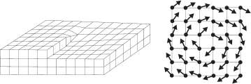
In Theorem 15 we prove the equivalence between the families of functionals $(\frac{GL_{\varepsilon}}{|\log\varepsilon|^{h}})$, $(\frac{XY_{\varepsilon}}{|\log\varepsilon|^{h}})$ and $(\frac{4\pi^{2}SD_{\varepsilon}}{|\log\varepsilon|^{h}})$ (see also Theorem 23 for $h=2$). The way our variational equivalence is proved provides an interesting identification between the order parameters and the corresponding singularities of the different models. For instance, the identification underlying the equivalence between $\frac{GL_{\varepsilon}}{|\log\varepsilon|^{h}}$ and $\frac{XY_{\varepsilon}}{|\log\varepsilon|^{h}}$ relies on suitable interpolation procedures which allow us to pass from the discrete order parameter of the $XY$ model to the continuous one of the $GL$ model. Analogously the displacement field in the $SD$ model is identified with the phase function of the $XY$ order parameter (see also Remark 2). These identifications of the order parameters clearly induce an identification of the corresponding singularities (see picture 1).

Refer to caption
Figure 1. A screw dislocation “corresponds” to a vortex of spins.

In the proof of Theorem 15, we have to make sure that the identification of the order parameters in the different models produces small perturbations in the corresponding free energy densities. This is easily checked far from the singularities, while to control the error near the singularities we need to introduce suitable reparametrizations ${\delta_{\varepsilon}}$ of the correlation length, i.e., we have to look at the models at suitable meso-scales ${\delta_{\varepsilon}}$. Finally, during these identifications, we have also to control the distance, measured in a suitable topology, of the corresponding singularities. This analysis involves notions of geometric measure theory, and the arguments used in the proofs are close to those used to prove density of polyhedral boundaries in the space of integer currents in [17] and also exploited in [1].

Taking advantage of this equivalence principle, we are able to export many of the known results in the theory of $GL$ vortices to the framework of $SD$ models. Indeed the $\Gamma$-convergence results in [23] in the $|\log\varepsilon|^{2}$ energetic regime, together with (2) for $h=2$, leads to new asymptotic results in the context of dislocations and spin systems when the number of defects grows logarithmically as $\varepsilon$ goes to zero (see Theorem 24).

The $|\log\varepsilon|^{2}$ energetic regime has been already considered in the vectorial context of homogenizing edge dislocations in [19], within a core radius approach, under the assumption that the dislocations have a minimal distance of the order of a suitable meso-scale. The $\Gamma$-convergence analysis done in [19] provides a macroscopic model for plasticity, in agreement with the phenomenological strain gradient theory for plasticity introduced in [18]. Moreover, the limit energy is compatible with the experimental evidence of the concentration of dislocations on lines, usually referred to as dislocation walls (we refer to [15] for a variational model describing dislocation patterns in crystals). In view of (2), we extend the $\Gamma$-convergence analysis done in [19] to our completely discrete setting, without any kinematic assumption on the mutual distance of the screw dislocations. In this way, we derive a strain gradient model for plasticity in the scalar setting of anti-planar elasticity, starting from a completely discrete and basic model of screw dislocations.

Finally, let us mention that, as a byproduct of our equivalence result (2), taking into account the $\Gamma$-convergence result proved in [30], we obtain (see Remark 18) a new proof of compactness and $\Gamma$-convergence for two-dimensional $GL$ functionals, independent of the proof given in [22] and in [32].

Our method can be clearly exploited in many interesting directions: first, one can investigate the equivalence of lower order terms for the models we have discussed so far, comparing the so called renormalized energy for vortices and dislocations within a $\Gamma$-convergence analysis, in the spirit of the theory of development by $\Gamma$-convergence introduced by Braides and Truvskinovsky in [12]. Moreover, one can consider the case of edge dislocations, or, more in general, the case of three dimensional models. Indeed, the results of this paper provide a first step in the effort of making a link between material dependent models for dislocations and phenomenological Ginzburg-Landau approaches. We believe that our arguments could give efficient hints to build up material dependent Ginzburg-Landau energies, taking into account kinematic constraints and elasticity constants specific of the crystal. Moreover, exploiting our variational equivalence arguments in the three dimensional problem (e.g., in a cubic crystal) would bring new light on interesting mathematical questions regarding compactness properties and asymptotic behaviour of generalized Ginzburg-Landau functionals, the target space being a three-dimensional torus, and the singularities being rectifiable currents with multiplicity in the group ${\mathbb{Z}}^{3}$ (see Section 7).

The paper is organized as follows. In Section 2 we introduce the discrete models for spin systems and screw dislocations, while in Section 3 we introduce the corresponding topological singularities. In Section 4 we describe our variational argument, that will be used in Section 5 to prove the variational equivalence between $GL_{\varepsilon}$, $XY_{\varepsilon}$ and $SD_{\varepsilon}$ models. Such an equivalence will be specialized in Section 6 in order to present new results in the asymptotic analysis of screw dislocations. In Section 7, we will comment the results achieved in this paper suggesting further extensions, concerning, for instance, the core radius approach to the singularities. Finally we will propose, in the case of three dimensional elasticity, a material dependent Ginzburg-Landau type model for dislocations in a cubic lattice.

2. Overview of the models

In this Section we briefly describe the models of Ginzburg-Landau vortices, of $XY$-spin systems and of screw dislocations. We will provide a detailed description of the latter in order to define the physical quantities involved in the model and needed to correctly describe the new results in the framework of screw dislocations contained in Section 6.

For the time being $\Omega\subset{\mathbb{R}}^{2}$ is a bounded open set with Lipschitz boundary, representing the domain of definition of the relevant fields in these models. For the sake of simplicity, we will also assume that $\Omega$ is star-shaped with respect to the origin. We stress that with some minor technical effort in our proofs, such assumption can be removed.

2.1. Ginzburg Landau functionals

Let us introduce the family of the so-called complex Ginzburg-Landau functionals $GL_{\varepsilon}:W^{1,2}(\Omega;{\mathbb{R}}^{2})\to[0,+\infty)$, defined as

(3) $$GL_{\varepsilon}(w):=\left(\int_{\Omega}\frac{1}{2}|\nabla w|^{2}+\frac{1}{\varepsilon^{2}}W(w)\right),$$

where $W(x):=(1-|x|)^{2}$. Here $w$ represents the order parameter of the model, describing how deep the material is in the superconductive phase, $\varepsilon$ is a length-scale parameter, usually referred to as the coherence length while $GL_{\varepsilon}$ is the corresponding free energy of the system.

Remark 1.

We make this explicit choice for $W=(1-|x|)^{2}$ because it simplifies some computation. The following standard hypotheses would suffice to perform our analysis: $W\in C({\mathbb{R}}^{2})$ such that $W(x)\geq 0$, $W^{-1}\{0\}=S^{1}$ and

$$\liminf\limits_{|x|\to 1}\frac{W(x)}{(1-|x|)^{2}}>0,\quad\liminf\limits_{|x|\to\infty}\frac{W(x)}{|x|^{2}}>0.$$

2.2. The discrete lattice

Here we introduce the discrete objects and notations we will use in the sequel.

For every positive $\varepsilon>0$, we set $\Omega_{\varepsilon}^{0}:=\varepsilon{\mathbb{Z}}^{2}\cap\Omega$, representing the reference lattice. We will denote by $\Omega_{\varepsilon}^{1}:=\{(i,j)\in\Omega_{\varepsilon}^{0}\times\Omega_{\varepsilon}^{0}:\,|i-j|=\varepsilon,\,i\leq j\}$ the class of nearest neighbors in $\Omega_{\varepsilon}^{0}$ (where $i\leq j$ means that $i_{l}\leq j_{l}$ for $l\in\{1,2\}$). The class of cells contained in $\Omega$ is labelled by the set $\Omega_{\varepsilon}^{2}:=\{i\in\Omega_{\varepsilon}^{0}:\,i+[0,\varepsilon]^{2}\subset\Omega\}$. Finally, we set

$$\Omega_{\varepsilon}:=\left\{\bigcup_{i\in\Omega_{\varepsilon}^{2}}i+[0,\varepsilon]^{2}\right\}.$$

In the following, we will extend the use of these notations to any given open subset $A$ of ${\mathbb{R}}^{2}$.

2.3. XY spin systems

Here we recall the model of $XY$ spin system following the approach in [3] (see also [34] for a general introduction to the model). First we introduce the class of admissible fields,

(4) $${\mathcal{AXY}_{\varepsilon}}:=\{v:\Omega_{\varepsilon}^{0}\to{\mathcal{S}}^{1}\},$$

where ${\mathcal{S}}^{1}$ denotes the set of unit vectors in ${\mathbb{R}}^{2}$. The family of functionals $XY_{\varepsilon}:{\mathcal{AXY}_{\varepsilon}}\to{\mathbb{R}}$ are defined by

(5) $$XY_{\varepsilon}(v):=\frac{1}{2}\sum_{(i,j)\in\Omega_{\varepsilon}^{1}}|{v(i)-v(j)}|^{2}.$$

We refer the interested reader to [3] for the derivation of these energies by proper scaling of the $XY$ energies written in the usual form

$$-\sum_{(i,j)\in\Omega_{\varepsilon}^{1}}\varepsilon^{2}\langle v(i),v(j)\rangle,$$

where $\langle a,b\rangle$ denotes the scalar product between the vectors $a$ and $b$.

2.4. Screw dislocations

Here we introduce a basic discrete model for screw dislocations, inspired by the approach introduced in [5] and revisited in [30]. The displacement, in this discrete anti-planar setting, is a function $u:\ \Omega_{\varepsilon}^{0}\to{\mathbb{R}}$. We denote the class of all admissible displacements by

(6) $${\mathcal{ASD}_{\varepsilon}}:=\{u:\Omega_{\varepsilon}^{0}\to{\mathbb{R}}\}.$$

We focus here on linearized elasticity, and we consider the model case of nearest neighbors interactions, so that the discrete elastic energy corresponding to any displacement $u$, in absence of dislocations, is given by (we fix the shear modulus $\mu=\frac{1}{2}$)

(7) $$E^{el}_{\varepsilon}(u):=\frac{1}{2}\sum_{(i,j)\in\Omega_{\varepsilon}^{1}}|u(i)-u(j)|^{2}.$$

It is convenient to introduce also the notion of discrete gradient ${\bf{d}}u$, defined on the nearest neighbors (namely, the bonds of the lattice), by ${\bf{d}}u_{i,j}=u(j)-u(i)$, for every $(i,j)\in\Omega_{\varepsilon}^{1}$. With respect to the discrete gradient ${\bf{d}}u$, the energy (7) reads like

(8) $$E^{el}_{\varepsilon}(u):=\frac{1}{2}\sum_{(i,j)\in\Omega_{\varepsilon}^{1}}|{\bf{d}}u_{i,j}|^{2}.$$

To introduce the dislocations in this framework, we adopt the point of view of the additive decomposition of the gradient of the displacement in an elastic part, the strain, and a plastic part, following the formalism of the discrete pre-existing strains as in [5] and [30]. More precisely, a pre-existing strain is a function $\beta^{p}$ representing the plastic part of the strain defined on pairs of nearest neighbors and valued in ${\mathbb{Z}}|b|$. Here $b$ represents the so called Burgers vector which is characteristic of the crystal. In principle $|b|$ should be of order $\varepsilon$, but up to a further re-scaling in the energy functionals, we can fix from now on $|b|=1$.

Here the idea is that the plastic strain $\beta^{p}$ does not store elastic energy and hence it has to be subtracted to the gradient of the displacement in order to obtain the so called elastic strain. In view of this additive decomposition $\nabla u=\beta^{p}+\beta^{e}$, we have that the elastic strain $\beta^{e}$ is not curl-free (in a suitable discrete sense). In Section 3 we will introduce the quantity $\mu:=\text{curl }\beta^{e}=-\text{curl }\beta^{p}$, that measures the degree of incompatibility of the elastic strain $\beta^{e}$ from being a discrete gradient, and represents the discrete screw dislocations in the crystal lattice.

Summarizing, the elastic energy corresponding to the decomposition $\nabla u=\beta^{p}+\beta^{e}$ is given by

$$E^{el}_{\varepsilon}(u):=\frac{1}{2}\sum_{(i,j)\in\Omega_{\varepsilon}^{1}}|\beta^{e}_{i,j}|^{2}=\frac{1}{2}\sum_{(i,j)\in\Omega_{\varepsilon}^{1}}|{\bf{d}}u_{i,j}-\beta^{p}_{i,j}|^{2},$$

and whenever the dislocation density $\text{curl }\beta^{e}=-\text{curl }\beta^{p}$ is non zero, then the corresponding elastic energy is also non zero.

Given a displacement $u$, we can minimize the corresponding elastic energy with respect to the plastic strain. Since by our kinematic assumption the plastic strain takes values in ${\mathbb{Z}}$, it is clear that the optimal $\beta_{u}^{p}$ is obtained projecting ${\bf d}u$ on ${\mathbb{Z}}$. More precisely, let $P:{\mathbb{R}}\to{\mathbb{Z}}$ be the projection operator defined by

(9) $$P(t)=\text{argmin}\{|t-s|,s\in{\mathbb{Z}}\},$$

with the convention that, if the argmin is not unique, then we choose that with minimal modulus. Then we have $\beta_{u}^{p}=P{\bf{d}}u$, in the sense that, for all $(i,j)\in\Omega_{\varepsilon}^{1}$, $(\beta_{u}^{p})_{i,j}=P({\bf{d}}u_{i,j})$. In this way, we obtain the elastic energy functionals $SD_{\varepsilon}:{\mathcal{ASD}_{\varepsilon}}\to{\mathbb{R}}$ defined by

(10) $$SD_{\varepsilon}(u):=\frac{1}{2}\sum_{(i,j)\in\Omega_{\varepsilon}^{1}}|(\beta_{u}^{e})_{i,j}|^{2}=\frac{1}{2}\sum_{(i,j)\in\Omega_{\varepsilon}^{1}}\text{dist}^{2}\big{(}u(i)-u(j),{\mathbb{Z}}\big{)}.$$

We notice that, defining $\tilde{u}:=\varepsilon u$ as the physical displacement, we have

$${\varepsilon^{2}SD_{\varepsilon}(u)}=\frac{1}{2}\sum_{(i,j)\in\Omega_{\varepsilon}^{1}}\text{dist}^{2}\big{(}\tilde{u}(i)-\tilde{u}(j),\varepsilon{\mathbb{Z}}\big{)},$$

where the r.h.s. now reads as a term penalizing a misfit slip in the crystal, according with Pierls-Nabarro theories.

Indeed, another way of understanding (10) is the following. In our anti-planar setting, the crystal can displace only in the vertical direction, and each vertical line of atoms has to displace rigidly. The discrete gradient ${\bf{d}}\tilde{u}$ measures the difference of the displacement of two near lines of atoms. If ${\bf{d}}\tilde{u}$ is of order $\varepsilon$, the periodic structure of the crystal is unperturbed, and therefore the corresponding stored energy has to vanish. In other words, the nearest neighbors interactions have to be labeled in the deformed configuration, and not in the reference one. The rigorous way of formalizing this idea is given exactly by the projection procedure introduced by the operator $P$ in (10).

Remark 2.

Here we describe the heuristic argument to identify the $XY$ and $SD$ models just introduced. The correspondence between the displacement functions $u_{\varepsilon}\in{\mathcal{ASD}_{\varepsilon}}$ and the $XY$ fields $v_{\varepsilon}\in{\mathcal{AXY}_{\varepsilon}}$ is given by identifying $u_{\varepsilon}$ with the phase function of $v_{\varepsilon}$. More precisely, given a displacement $u_{\varepsilon}\in{\mathcal{ASD}_{\varepsilon}}$, the corresponding field $v(u_{\varepsilon})$ for the $XY$ model is given by

(11) $$v(u_{\varepsilon})(l):=e^{2\pi iu_{\varepsilon}(l)}\qquad\text{ for every }l\in\Omega_{\varepsilon}^{0}.$$

Viceversa, given $v_{\varepsilon}\in{\mathcal{AXY}_{\varepsilon}}$, the corresponding displacement is $u(v_{\varepsilon}):=\tfrac{1}{2\pi}\theta_{v_{\varepsilon}}$, where $\theta_{v_{\varepsilon}}\in[0,2\pi)$ is defined by the identity $v_{\varepsilon}=e^{i\theta_{v_{\varepsilon}}}$. Note that the (arbitrary) choice of a precise representative of the phase $\theta_{v_{\varepsilon}}$ of $v_{\varepsilon}$ does not affect the elastic energy corresponding to $u(v_{\varepsilon})$. Indeed, we have

$$2\pi\,\text{dist}(u_{\varepsilon}(i)-u_{\varepsilon}(j),{\mathbb{Z}})=d_{S^{1}}(v(u_{\varepsilon})(i)-v(u_{\varepsilon})(j)),$$

where $d_{S^{1}}$ denotes the geodesic distance on $S^{1}$.

Finally, we notice that by Taylor expansion we have $2\pi(u_{\varepsilon}(i)-u_{\varepsilon}(j))\approx v(u_{\varepsilon})(i)-v(u_{\varepsilon})(j)$, whenever $u_{\varepsilon}(i)-u_{\varepsilon}(j)$ is small. Therefore, we expect the identification between the fields to produces small perturbations in the corresponding energy densities (up to a pre-factor $4\pi^{2}$) far from the singularities, and this will be formalized in the sequel.

3. The topological singularities and energy functionals

As discovered by Jerrard in [21] (see also [22]), the Jacobian of the order parameter is the relevant geometric object carrying energetic informations for the Ginzburg-Landau functionals. In the same spirit, in this paper we introduce suitable discrete notions for the topological singularities of the models we have introduced, and we consider them as the meaningful variables of the corresponding discrete energy functionals.

For the $SD$ model, the topological singularity is given by the discrete dislocation, defined through a discrete version of the curl of the elastic strain, while for $XY$ spin systems, the natural notion of topological singularity is that of discrete vortex, that we will introduce in the sequel.

We will follow the formalism introduced in [5] (see also [30]) representing the singularities by a discrete function $\alpha$ whose values on the cells of the lattice represent the topological degree of the singularity. Moreover, we will identify this function $\alpha$ with a measure concentrated on the center of the cells of the lattice.

As we will see in the sequel, we can always pass from a discrete representation of the singularities to a continuous one (and viceversa) by mean of interpolations procedures (and projection on finite elements space respectively). This will also be consistent with the topology we are going to use to perform the $\Gamma$-convergence analysis: the distance, measured in such a topology, between the continuous representation of the singularities and its discrete counterpart will turn out to be vanishing for sequences of order parameters with bounded energy (see Proposition 16).

3.1. The Jacobian

Given $w\in H^{1}(\Omega;{\mathbb{R}}^{2})$, the Jacobian of $w$ is the $L^{1}$ function defined by

$$Jw:=\text{det}\nabla v.$$

Let us denote by $C^{0,1}_{c}(\Omega)$ the space of Lipschitz continuous functions on $\Omega$ with compact support, and by $X$ its dual. The dual norm of $X$ will be denoted by $\|\cdot\|$.

For every $w\in H^{1}(\Omega;{\mathbb{R}}^{2})$, we can consider $Jw$ as an element of $X$ by setting

$$<Jw,\varphi>:=\int_{\Omega}Jw\,\varphi\,dx\qquad\text{ for every }\varphi\in C^{0,1}_{c}({\Omega}).$$

Note that $Jw$ can be written (in the sense of distributions) in a divergence form as

(12) $$Jw=\text{div }(w_{1}(w_{2})_{x_{2}},-w_{1}(w_{2})_{x_{1}}),$$

or equivalently, in the form $Jw=\text{curl }(w_{1}\nabla w_{2})$. By a density argument, we deduce that for every $\varphi\in C^{0,1}_{c}(\Omega)$,

(13) $$<Jw,\varphi>=-\int_{{\mathbb{R}}^{2}}w_{1}(w_{2})_{x_{2}}\varphi_{x_{1}}-w_{1}(w_{2})_{x_{1}}\varphi_{x_{2}}\,dx.$$

Note that the right hand side of (13) is well defined also when

$$w\in W^{1,1}(\Omega;{\mathbb{R}}^{2})\cap L^{\infty}(\Omega;{\mathbb{R}}^{2}),$$

and for such a function, we will take (13) as the definition of $Jw$ as an element of $X$.

Finally, for later use we notice that for every $v:=(v_{1},v_{2}),\,w:=(w_{1},w_{2})$ belonging to $H^{1}(\Omega;{\mathbb{R}}^{2})$ (or, as well, to $W^{1,1}(\Omega;{\mathbb{R}}^{2})\cap L^{\infty}(\Omega;{\mathbb{R}}^{2})$), we have

(14) $$Jv-Jw=\frac{1}{2}\big{(}J(v_{1}-w_{1},v_{2}+w_{2})-J(v_{2}-w_{2},v_{1}+w_{1})\big{)}.$$

By (13) and (14) we immediately deduce the following lemma.

Lemma 3.

Let $v_{n}$ and $w_{n}$ be two sequences in $H^{1}(\Omega;{\mathbb{R}}^{2})$ such that

$$\|v_{n}-w_{n}\|_{2}(\|\nabla v_{n}\|_{2}+\|\nabla w_{n}\|_{2})\to 0.$$

Then $\|Jv_{n}-Jw_{n}\|\to 0$ in $X$.

3.2. Discrete dislocations

Following the formalism introduced in [5] (see also [30]), given a function $\xi:\Omega_{\varepsilon}^{1}\to{\mathbb{R}}$ (playing the role of a pre-existing strain), we introduce its discrete curl ${\bf{d}}\xi:\Omega_{\varepsilon}^{2}\to{\mathbb{R}}$, defined for every $i\in\Omega_{\varepsilon}^{2}$ by

(15) $${\bf{d}}\xi(i):=\xi_{i,i+(0,\varepsilon)}+\xi_{i+(0,\varepsilon),i+(\varepsilon,\varepsilon)}-\\ \xi_{i+(\varepsilon,0),i+(\varepsilon,\varepsilon)}-\xi_{i,i+(\varepsilon,0)}.$$

Given an admissible displacement $u:\Omega_{\varepsilon}^{0}\to{\mathbb{R}}$, we recall that we can decompose ${\bf{d}}u$ in its elastic and plastic part (that is optimal in energy), by setting $\beta_{u}^{p}=P{\bf{d}}u$, $\beta_{u}^{e}={\bf{d}}u-\beta^{p}_{u}$, where $P$ is defined in (9).

We are now in a position to introduce the discrete dislocation function $\alpha_{u}:\Omega_{\varepsilon}^{2}\to\{-1,\,0,\,1\}$, defined by

$$\alpha_{u}(i):={\bf{d}}\beta_{u}^{e}(i)\qquad\text{ for every }i\in\Omega_{\varepsilon}^{2}.$$

It will be convenient also to represent $\alpha_{u}$ as a sum of Dirac masses with weights in $\{-1,\,0,\,1\}$ and supported on the centers of the squares where $\alpha\neq 0$, setting

(16) $$\mu_{u}:=\sum_{i\in\Omega_{\varepsilon}^{2}}\alpha_{u}(i)\delta_{i+\frac{1}{2}(\varepsilon,\varepsilon)}.$$
Remark 4.

Notice that, in view of the very definition of $P$, we have that $\beta_{u}^{e}\in(-1/2,\,1/2]$, therefore by definition (15) the discrete dislocation $\alpha_{u}$ takes values in $\{-1,\,0,\,1\}$. We deduce that, in our model, only singular dislocations can be present in a cell.

3.3. Discrete vortices

Given an admissible field $v\in{\mathcal{AXY}_{\varepsilon}}$, the associated discrete vorticity $\gamma_{v}:\Omega_{\varepsilon}^{2}\to{\mathbb{Z}}$ is defined by

(17) $$\gamma_{v}:=\alpha_{\tfrac{1}{2\pi}\theta(v)},$$

where $\theta(v)\in[0,2\pi)$ is the phase of $v$ defined by the relation $v=e^{i\theta(v)}$. Moreover, we introduce the measure $\mu_{v}$ defined by

(18) $$\mu_{v}:=\sum_{i\in\Omega_{\varepsilon}^{2}}\gamma_{v}(i)\delta_{i+\frac{1}{2}(\varepsilon,\varepsilon)}.$$

Notice that, as for the screw dislocations, in a cell we can have only singular vortices.

Remark 5.

Given $v\in{\mathcal{AXY}_{\varepsilon}}$, we can introduce a function $\tilde{v}:\Omega_{\varepsilon}\to{\mathbb{R}}^{2}$ that coincides with $v$ on $\Omega_{\varepsilon}^{0}\cap\Omega_{\varepsilon}$ and such that $J\tilde{v}=\pi\mu_{v}$. Indeed, consider the function $\tilde{\theta}(v)$ defined on each segment $[i,j]$ with $(i,j)\in\Omega_{\varepsilon}^{1}$ by

$$\tilde{\theta}(v)(i+s(j-i))=\theta(v)(i)+2\pi s\,(\beta^{e}_{u(v)})_{i,j}\qquad\text{ for every }s\in[0,1],$$

where $u(v):=\tfrac{1}{2\pi}\theta(v)$. Now, extend $\tilde{\theta}(v)$ in each cell $i+[0,\varepsilon]^{2}$ (with $i\in\Omega_{\varepsilon}^{2}$), making it zero-homogeneous with respect to the center of the cell. Finally, on each cell we set $\tilde{v}:=e^{i\tilde{\theta}(v)}$.

A straightforward computation leads to the equality $J\tilde{v}=\pi\mu_{v}$. This argument shows that the vorticity function $\alpha_{v}$ represents a discrete version of the Jacobian, and seems a very natural object in this context.

Finally, for latter use, we notice that it can be easily proved (for instance by the identity $J\tilde{v}=\text{curl }(\tilde{v}_{1}\nabla\tilde{v}_{2})$) that for each $\varepsilon$-square $Q_{i}$ with $i\in\Omega_{\varepsilon}^{2}$ we have

(19) $$\mu_{v}(Q_{i})=\frac{1}{\pi}\int_{\partial Q_{i}}\tilde{v}_{1}\frac{\partial}{\partial s}\tilde{v}_{2}\,ds.$$
Remark 6.

We notice here that a very easy estimate leads to the following bound for the total variation of the topological singularities

$$|Jw_{\varepsilon}|(\Omega)\leq C\,GL_{\varepsilon}(w_{\varepsilon}),\quad|\mu_{v_{\varepsilon}}|(\Omega)\leq C\,XY_{\varepsilon}(v_{\varepsilon}),\quad|\mu_{u_{\varepsilon}}|(\Omega)\leq C\,SD_{\varepsilon}(u_{\varepsilon}).$$

3.4. The energy functionals

In this paragraph we will formally introduce the (rescaled) energy functionals corresponding to the $XY$ spin system, the screw dislocations and the Ginzburg-Landau models written in terms of the corresponding singularities.

In order to rewrite the energy functionals in these new variables, we minimize the free energies among all field quantities compatible with the prescribed singularity. For instance, in the $SD$ model, we will fix $\mu:=\text{curl }\beta^{e}$, and minimize the elastic energy among all $u$ compatible with $\mu$, i.e., with $\mu_{u}=\mu$. The corresponding energy functional can be thought of as the energy stored in the crystal, for a certain given dislocation density.

We will consider the energetic regimes of order $|\log\varepsilon|^{h}$, where $h$ is any fixed positive real number. Following the convention according to which the infimum of the empty set is $+\infty$, we define the Ginzburg-Landau energy functional $\mathcal{GL}_{\varepsilon}:X\to[0,+\infty]$, where $X=(C^{0,1}_{c}(\Omega))^{*}$, as

(20) $$\mathcal{GL}_{\varepsilon}(\mu):=\frac{1}{|\log\varepsilon|^{h}}\inf\left\{GL_{\varepsilon}(w),w\in H^{1}({\Omega};{\mathbb{R}}^{2}):\frac{J(w)}{\pi|\log\varepsilon|^{h-1}}=\mu\right\}.$$

Let us pass to the energy functionals corresponding to $XY$ spin systems. Using the notations introduced in the Section 3, the energy functionals $\mathcal{XY}_{\varepsilon}:X\to[0,+\infty]$ are defined by

(21) $$\mathcal{XY}_{\varepsilon}(\mu):=\frac{1}{|\log\varepsilon|^{h}}\inf\left\{XY_{\varepsilon}(v),\,v\in{\mathcal{AXY}_{\varepsilon}}:\frac{\mu_{v}}{|\log\varepsilon|^{h-1}}=\mu\right\}.$$

Finally the energy functionals corresponding to the screw dislocations model $\mathcal{SD}_{\varepsilon}:X\to[0,+\infty]$ are defined by

(22) $$\mathcal{SD}_{\varepsilon}(\mu):=\frac{4\pi^{2}}{|\log\varepsilon|^{h}}\inf\left\{SD_{\varepsilon}(u),\,u\in{\mathcal{ASD}_{\varepsilon}}:\frac{\mu_{u}}{|\log\varepsilon|^{h-1}}=\mu\right\},$$

where the prefactor $4\pi^{2}$ is just a normalization factor which guarantees that the family $(\mathcal{SD}_{\varepsilon})$ asymptotically behaves as $\mathcal{XY}_{\varepsilon}$ and $\mathcal{GL}_{\varepsilon}$.

4. The variational equivalence argument

In this section we will introduce a notion of equivalence between families of functionals defined on a metric space $(X,d)$, depending on a small parameter $\varepsilon$. Such a notion turns out to be efficient to compare different variational models which share the same asymptotic behavior as $\varepsilon$ goes to zero.

4.1. The notion of variational equivalence

Let $(F_{\varepsilon})$ and $(G_{\varepsilon})$ be two families of functionals from $X$ to ${\mathbb{R}}\cup\{\infty\}$ depending on the parameter $\varepsilon\in{\mathbb{R}}^{+}\cup\{0\}$.

Definition 7.

We set $(G_{\varepsilon})\preceq(F_{\varepsilon})$ if there exists a continuous increasing function $\varepsilon\mapsto\delta_{\varepsilon}$, with $\delta_{0}=0$, such that the following holds.

For every $\varepsilon_{n}\to 0$, and $(p_{n})\subset X$ such that $F_{{\varepsilon_{n}}}(p_{n})\leq C$, there exists a family $(q_{n})\subset X$ such that

  • i)

    $\limsup_{n}(G_{\delta_{{\varepsilon_{n}}}}(q_{n})-F_{{\varepsilon_{n}}}(p_{n}))\leq 0$;

  • ii)

    Either $(p_{n})$ and $(q_{n})$ are unbounded or $d(p_{n},q_{n})\to 0$ as $n\to+\infty$.

We set $(F_{\varepsilon})\simeq(G_{\varepsilon})$, and we say that $(F_{\varepsilon})$ and $(G_{\varepsilon})$ are variationally equivalent (for $\varepsilon\to 0$) if $(F_{\varepsilon})\preceq(G_{\varepsilon})$ and $(G_{\varepsilon})\preceq(F_{\varepsilon})$.

Note that the relation $\preceq$ just introduced is transitive, i.e., if $F^{1}_{\varepsilon}\preceq F^{2}_{\varepsilon}$ and $F^{2}_{\varepsilon}\preceq F^{3}_{\varepsilon}$ then $F^{1}_{\varepsilon}\preceq F^{3}_{\varepsilon}$. Moreover the relation $\simeq$ is an equivalence relation between families of functionals $\{(F_{\varepsilon}),F_{\varepsilon}:X\to{\mathbb{R}}\}$, i.e., the following properties hold

Reflexivity: $\displaystyle(F_{\varepsilon})\simeq(F_{\varepsilon});$
Symmetry: $\displaystyle(F_{\varepsilon})\simeq(G_{\varepsilon})\text{ implies }(G_{\varepsilon})\simeq(F_{\varepsilon});$
Transitivity: $\displaystyle(F_{\varepsilon})\simeq(G_{\varepsilon})\text{ and }(G_{\varepsilon})\simeq(H_{\varepsilon})\text{ imply }(G_{\varepsilon})\simeq(H_{\varepsilon}).$

4.2. Some consequences of the variational equivalence

Let us consider now a first important relation between the notion of variational equivalence and that of $\Gamma$-convergence (for the definition and the main properties of $\Gamma$-convergence we refer the reader to [10] and [16]). To this purpose we recall the following definition of equi-coercivity: a family of functionals $(F_{\varepsilon})$ is said to be equi-coercive if, given ${\varepsilon_{n}}\to 0$ and $(p_{n})$ such that $F_{{\varepsilon_{n}}}(p_{n})<C$, then $(p_{n})$ is relatively compact in $X$.

Theorem 8.

Let $(F_{\varepsilon})$ be a family of equi-coercive functionals $\Gamma$-converging to some functional $H$ in $X$. Then $(F_{\varepsilon})$ is variationally equivalent to the constant sequence $H_{\varepsilon}\equiv H$.

Proof.

We begin proving $F_{\varepsilon}\preceq H$ by a contradiction argument. Assume by contradiction that the relation $F_{\varepsilon}\preceq H$ does not hold; then there exist sequences ${\varepsilon_{n}}\to 0$, $(p_{n})\subset X$ with $H(p_{n})\leq C$, and $r>0$ such that

(23) $$\inf_{x\in B_{r}(p_{n})}F_{\varepsilon_{n}}(x)\geq H(p_{n})+r.$$

On the other hand, by the equi-coercivity of $F_{\varepsilon}$ we easily deduce the coercivity of $H$, so that we can assume without loss of generality that $p_{n}$ converges to some $p\in X$. By the $\Gamma$-limsup inequality there exists a sequence $(z_{n})\subset X$ such that

(24) $$z_{n}\to p,\qquad F_{\varepsilon_{n}}(z_{n})\to H(p)\leq\liminf H(p_{n}).$$

Equation (23) together with (24) provides a contradiction.

Let us pass to the proof of the opposite inequality $H\preceq F_{\varepsilon}$. Assume by contradiction that there exist sequences ${\varepsilon_{n}}\to 0$, $(p_{n})\subset X$ with $F_{{\varepsilon_{n}}}(p_{n})\leq C$ and $r>0$ such that

(25) $$\inf_{x\in B_{r}(p_{n})}H(x)\geq F_{{\varepsilon_{n}}}(p_{n})+r.$$

By the equi-coercivity property of $F_{\varepsilon}$ we may assume that $p_{n}\to p$ in X, and by the $\Gamma$-liminf inequality we have that, for n big enough

$$\inf_{x\in B_{r}(p_{n})}H(x)\leq H(p)\leq\liminf F_{{\varepsilon_{n}}}(p_{n}),$$

which, together with (25) provides a contradiction. ∎

Remark 9.

Note that in Theorem 8 the equicoercivity assumption plays a fundamental role. Indeed consider the space $l_{2}$ of sequences $\{a_{i}\}$ with $\sum_{i}a_{i}^{2}$ finite, and consider the functionals $F_{\varepsilon}:{\mathbb{R}}\to{\mathbb{R}}$ defined by

$$F_{\varepsilon}(\{a_{i}\}):=\sum_{i\neq[1/\varepsilon]}a_{i}^{2},$$

where $[1/\varepsilon]$ denotes the integer part of $1/\varepsilon$. Clearly $F_{\varepsilon}$ $\Gamma$-converge to the functional $H(\{a_{i}\}):=\|\{a_{i}\}\|_{2}^{2}$, but $F_{\varepsilon}$ is not variationally equivalent to $H$.

The next theorem, together with Theorem 8, clarifies the relation between the notion of $\Gamma$-convergence and the notion of variational equivalence.

Theorem 10.

Let $(F_{\varepsilon})$ and $(G_{\varepsilon})$ be variationally equivalent. Then the following properties hold.

  • 1)

    $F_{\varepsilon}$ are equi-coercive if and only if $G_{\varepsilon}$ are equi-coercive;

  • 2)

    $F_{\varepsilon}$ $\Gamma$-converge to some functional $H$ in $X$ if and only if $G_{\varepsilon}$ $\Gamma$-converge to $H$.

Proof.

To prove property $1)$ assume for instance that $G_{\varepsilon}$ are equi-coercive and let us prove that so are also $F_{\varepsilon}$. To this aim let $\varepsilon\mapsto\delta_{\varepsilon}$ be the map given in the definition of $G_{\varepsilon}\preceq F_{\varepsilon}$. Let ${\varepsilon_{n}}\to 0$ and $(p_{n})\subset X$ be such that $F_{{\varepsilon_{n}}}(p_{n})\leq C$. By Definition 7 there exists a sequence $(q_{n})\subset X$ such that $\limsup_{n}G_{\delta_{{\varepsilon_{n}}}}(q_{n})\leq C$. By the equi-coercivity property of $G_{\varepsilon}$ we deduce that (up to a subsequence) $q_{n}\to x$ for some $x\in X$. By property $ii)$ of Definition 7 we deduce that $d(p_{n},q_{n})\to 0$ and therefore that $p_{n}\to x$.

Let us pass to property 2). Assume for instance that $F_{\varepsilon}$ $\Gamma$-converge to $H$ and let us prove that also $G_{\varepsilon}$ $\Gamma$-converge to $H$. To this purpose, let ${\varepsilon_{n}}\to 0$ and let $\rho_{n}$ be such that ${\varepsilon_{n}}=\delta_{\rho_{n}}$. In order to prove the $\Gamma$-limsup inequality let $p\in X$, and let $(p_{n})$ be a recovery sequence for $F_{\rho_{n}}$; i.e., $p_{n}\to p$ and $F_{\rho_{n}}(p_{n})\to F(p)$. Consider the sequences $(q_{n})\subset X$ given by Definition 7. By property ii) of Definition 7 we have that $q_{n}\to p$, and by property i) we have that

$$\limsup G_{{\varepsilon_{n}}}(q_{n})\leq\lim_{n}F_{\rho_{n}}(p_{n})=H(p).$$

In order to prove the $\Gamma$-liminf inequality, let now $\varepsilon\to{\delta_{\varepsilon}}$ be the map given in the definition of $F_{\varepsilon}\preceq G_{\varepsilon}$ and let $p_{n}\to p$. By Definition 7 there exists a sequence $q_{n}\to p$ such that

$$H(p)\leq\liminf_{n}F_{\delta_{{\varepsilon_{n}}}}(q_{n})\leq\liminf_{n}G_{{\varepsilon_{n}}}(p_{n}),$$

that proves the $\Gamma$-liminf inequality. ∎

Remark 11.

Note that if $F_{\varepsilon}$ and $G_{\varepsilon}$ are variationally equivalent, by Theorem 10 we deduce that they share the same $\Gamma$-limits even when they are not equi-coercive.

We also notice that in the class of equi-coercive functionals admitting a $\Gamma$-limit, our definition of equivalence coincides with that given (at order zero) in [12].

Remark 12.

Even if Definition 7 is given in a metric context, it can be generalized to vectorial topological spaces. We chose the metric framework because it is usually general enough for practical applications, the metric $d$ being either the metric inducing the weak topology of a ball in a Banach space, or (in view of a compact embedding) the distance induced by the norm of a Banach space.

4.3. A first example of equivalent families

For all positive $s>0$ consider the Ginzburg-Landau functionals $GL^{s}_{\varepsilon}:W^{1,2}(\Omega;{\mathbb{R}}^{2})\to[0,+\infty)$, defined as

(26) $$GL^{s}_{\varepsilon}(w):=\frac{1}{2}\int_{{{\mathbb{R}}^{2}}}|\nabla w|^{2}+\frac{s}{\varepsilon^{2}}W(w).$$

Note that for $s=1$ the functionals $GL^{s}_{\varepsilon}$ coincides with the functional $GL_{\varepsilon}$ defined in (3). Consider also the functional $\mathcal{GL}_{\varepsilon}^{s}:X\to[0,+\infty]$ defined as in (20) with $GL_{\varepsilon}$ replaced by $GL^{s}_{\varepsilon}$.

Proposition 13.

For every $0<s_{1}<s_{2}$, the families of functionals $\mathcal{GL}_{\varepsilon}^{s_{1}}$ and $\mathcal{GL}_{\varepsilon}^{s_{2}}$ are variationally equivalent, according to Definition 7.

Proof.

Let $s_{1}<s_{2}$. Since $\mathcal{GL}_{\varepsilon}^{s_{1}}\leq\mathcal{GL}_{\varepsilon}^{s_{2}}$, we immediately deduce $\mathcal{GL}_{\varepsilon}^{s_{1}}\preceq\mathcal{GL}_{\varepsilon}^{s_{2}}$. In order to prove the opposite relation, consider the following change of variables

$$\varepsilon{\mapsto}{\delta_{\varepsilon}}:=\varepsilon\left(\frac{s_{2}}{s_{1}}\right)^{\frac{1}{2}}.$$

Following Definition 7, let $\varepsilon_{n}\to 0$ as $n\to+\infty$ and let $(p_{n})\subset X$ be such that $\mathcal{GL}_{\varepsilon_{n}}^{s_{1}}(p_{n})\leq C$. Moreover, set

$$t_{n}:=\tfrac{|\log{\delta_{\varepsilon_{n}}}|^{h-1}}{|\log\varepsilon_{n}|^{h-1}},\qquad q_{n}:=\frac{p_{n}}{t_{n}}.$$

By the fact that $t_{n}\to 1$ as $n\to+\infty$ it immediately follows that either $p_{n}$ and $q_{n}$ are both unbounded or $d(p_{n},q_{n})\to 0$.

Let $(w_{n})\subset H^{1}({{\mathbb{R}}^{2}};{\mathbb{R}}^{2})$ be such that

$$\frac{1}{|\log\varepsilon_{n}|^{h-1}}Jw_{n}=p_{n},\qquad\tfrac{1}{|\log\varepsilon_{n}|^{h}}GL^{s_{1}}_{\varepsilon_{n}}(w_{n})-\mathcal{GL}^{s_{1}}_{\varepsilon_{n}}(p_{n})\to 0\text{ as }n\to+\infty.$$

Then, since by construction $\tfrac{1}{|\log{\delta_{\varepsilon_{n}}}|^{h-1}}Jw_{n}=q_{n}$, we have

$$\limsup_{n}(\mathcal{GL}_{\delta_{\varepsilon_{n}}}^{s_{2}}(q_{n})-\mathcal{GL}_{\varepsilon_{n}}^{s_{1}}(p_{n}))\\ \leq\limsup_{n}\left(\frac{1}{|\log{\delta_{\varepsilon_{n}}}|^{h}}GL_{\delta_{\varepsilon_{n}}}^{s_{2}}(w_{n})-\frac{1}{|\log{\varepsilon_{n}}|^{h}}GL_{\varepsilon_{n}}^{s_{1}}(w_{n})\right)\\ =\limsup_{n}\Big{(}\frac{1}{|\log\left(\varepsilon_{n}\frac{s_{2}}{s_{1}}\right)^{\frac{1}{2}}|^{h}}-\frac{1}{|\log\varepsilon_{n}|^{h}}\Big{)}\left(\frac{1}{2}\int_{{{\mathbb{R}}^{2}}}|\nabla w_{n}|^{2}+\frac{s_{1}}{\varepsilon_{n}^{2}}W(w_{n})\right)=0.$$

In the following we will need a slight variant of Proposition 13, where the pre-factor $s$ in front of the potential term $W$ is a suitable function of $\varepsilon$.

Proposition 14.

Let $\varepsilon\mapsto s_{\varepsilon}$ be an increasing functions from ${\mathbb{R}}^{+}$ to ${\mathbb{R}}^{+}$ such that $\tfrac{|\log s_{\varepsilon}|}{|\log\varepsilon|}\to 0$ as $\varepsilon\to 0$. Then the functionals $\mathcal{GL}_{\varepsilon}$ are variationally equivalent to $\mathcal{GL}^{s_{\varepsilon}}_{\varepsilon}$, according to Definition 7.

Proof.

The proof follows the lines of the proof of Proposition 13, setting now ${\delta_{\varepsilon}}:=\tfrac{\varepsilon}{\sqrt{s_{\varepsilon}}}$. ∎

5. Variational equivalence between $\mathcal{GL}_{\varepsilon}$, $\mathcal{XY}_{\varepsilon}$ and $\mathcal{SD}_{\varepsilon}$

In this Section we prove the main result of the paper: the energies corresponding to $XY$ spin systems, to screw dislocations and to the Ginzburg-Landau model are variationally equivalent in the sense of Definition 7. We prove this result for any scaling of the energies of order $|\log\varepsilon|^{h}$ with $h\geq 1$, the most relevant cases being $h=1$ and $h=2$.

In order to define all the energy functionals in the same space, we consider the Banach space $(X,\|\cdot\|)$ defined as the dual of Lipschitz functions with compact support in $\Omega$, endowed with the dual norm. This space is the natural space for the topological singularities, that are the relevant quantities in all the investigated models. The functionals $\mathcal{GL}_{\varepsilon}$, $\mathcal{XY}_{\varepsilon}$ and $\mathcal{SD}_{\varepsilon}$ from $X$ to $[0,+\infty]$ are defined rigorously in (20), (21) and (22) respectively.

Theorem 15.

The functionals $\mathcal{XY}_{\varepsilon}$, $\mathcal{SD}_{\varepsilon}$ and $\mathcal{GL}_{\varepsilon}$ are variationally equivalent according to Definition 7.

We will prove in three steps that $\mathcal{XY}_{\varepsilon}\preceq\mathcal{GL}_{\varepsilon}\preceq\mathcal{SD}_{\varepsilon}\preceq\mathcal{XY}_{\varepsilon}$. This relations imply the equivalence of all the functionals by the transitivity property of the order relation $F\preceq G$. Before the proof of Theorem 15 we state and prove a proposition that will be used to identify the discrete description of the singularities (i.e., the discrete measures $\mu_{u}$ and $\mu_{v}$ defined in (16) and (18), respectively) with the diffuse Jacobians of some suitable interpolation of the corresponding fields. To this purpose, for every positive $\varepsilon>0$, consider the triangulation ${\mathcal{T}}_{\varepsilon}:=\{T^{\pm}(i),\,i\in\varepsilon{\mathbb{Z}}^{2}\}$ whose triangles are of the type

(27) $\displaystyle T^{-}(i):=\{(x_{1},x_{2}):i_{1}\leq x_{1}\leq i_{1}+\varepsilon,\,i_{2}\leq x_{2}\leq i_{2}+x_{1}\};$
(28) $\displaystyle T^{+}(i):=\overline{(i_{1},i_{1}+\varepsilon)\times(i_{2},i_{2}+\varepsilon)\setminus T^{-}_{\varepsilon}(i)}.$

To any $v_{\varepsilon}$ in ${\mathcal{AXY}_{\varepsilon}}$, we can associate the continuous field $w(v_{\varepsilon})$ in $H^{1}(\Omega_{\varepsilon};{\mathbb{R}}^{2})$ given by the piece-wise linear interpolation of $v_{\varepsilon}$ on the triangles of ${\mathcal{T}}_{\varepsilon}$ contained in $\Omega_{\varepsilon}$. Note that the Jacobian of $w(v_{\varepsilon})$ is piecewise constant and that it can be extended by zero to a $L^{1}$ function in $\Omega$. Therefore $J(w(v_{\varepsilon}))$ can be seen as an element of $X$.

Since we will need to localize the energy functionals to subsets of $\Omega$, we introduce the following notation. Given $A\subset\Omega$, we will denote by $GL_{\varepsilon}(\cdot,A)$ the restriction of the $GL_{\varepsilon}$ energy density to $A$, and we denote by $XY_{\varepsilon}(\cdot,A)$ and $SD_{\varepsilon}(\cdot,A)$ the restriction of the corresponding energy densities to the nearest neighbors contained in $A$. Finally, for every given positive $\delta$ we set

(29) $$I_{\delta}(\Omega):=\{x\in\Omega:\min_{y\in\partial\Omega}\min_{i\in\{1,2\}}|x_{i}-y_{i}|>\delta\}.$$
Proposition 16.

Let $v_{\varepsilon}\in{\mathcal{AXY}_{\varepsilon}}$ be a sequence with $XY_{\varepsilon}(v_{\varepsilon})\leq C|\log\varepsilon|^{h}$. Then $\|\frac{Jw(v_{\varepsilon})}{\pi}-\mu_{v_{\varepsilon}}\|\to 0$ as $\varepsilon\to 0$.

Proof.

Let ${\delta_{\varepsilon}}:=\left(\varepsilon|\log\varepsilon|^{h+1}\right)$, denote by $\tilde{\delta_{\varepsilon}}$ the projection of ${\delta_{\varepsilon}}$ on $\varepsilon{\mathbb{Z}}$, and set

$\displaystyle R^{h}_{\tilde{\delta_{\varepsilon}}}:=\{(x,y)\in{\mathbb{R}}^{2}:y\in\tilde{\delta_{\varepsilon}}{\mathbb{Z}}\},$
$\displaystyle R^{v}_{\tilde{\delta_{\varepsilon}}}:=\{(x,y)\in{\mathbb{R}}^{2}:x\in\tilde{\delta_{\varepsilon}}{\mathbb{Z}}\},$
$\displaystyle R_{\tilde{\delta_{\varepsilon}}}:=(R^{h}_{\tilde{\delta_{\varepsilon}}}\cup R^{v}_{\tilde{\delta_{\varepsilon}}})\cap I_{\tilde{\delta_{\varepsilon}}}(\Omega).$

If we denote by $R^{1}_{\tilde{\delta_{\varepsilon}}}(s)$ the class of nearest neighbors in $R_{\tilde{\delta_{\varepsilon}}}+(s,s)$, by the Mean Value Theorem it is easy to prove that there exists $s_{\tilde{\delta_{\varepsilon}}}\in\varepsilon\{0,1,\ldots,\tfrac{\tilde{\delta_{\varepsilon}}}{\varepsilon}\}$ such that

$\displaystyle XY_{\varepsilon}(v_{\varepsilon})\geq$ $\displaystyle\sum\limits_{s\in\varepsilon\{0,1,\ldots,\tfrac{\tilde{\delta_{\varepsilon}}}{\varepsilon}\}}\sum_{l,k\in R_{\tilde{\delta_{\varepsilon}}}^{1}(s)}\frac{1}{2}|v_{\varepsilon}(l)-v_{\varepsilon}(k)|^{2}$
(30) $\displaystyle\geq$ $\displaystyle\frac{\tilde{\delta_{\varepsilon}}}{\varepsilon}\sum_{l,k\in R_{\tilde{\delta_{\varepsilon}}}^{1}(s_{\tilde{\delta_{\varepsilon}}})}\frac{1}{2}|v_{\varepsilon}(l)-v_{\varepsilon}(k)|^{2}.$

By (5) we deduce that

$$\max_{l,k\in R_{\tilde{\delta_{\varepsilon}}}^{1}(s_{\tilde{\delta_{\varepsilon}}})}|v_{\varepsilon}(l)-v_{\varepsilon}(k)|\to 0\qquad\text{ as }\varepsilon\to 0.$$

Let us denote by $Q_{\tilde{\delta_{\varepsilon}}}^{i}$ the cubes contained in $I_{\tilde{\delta_{\varepsilon}}}(\Omega)+(s_{\tilde{\delta_{\varepsilon}}},s_{\tilde{\delta_{\varepsilon}}})$ of the type

$$Q_{\tilde{\delta_{\varepsilon}}}^{i}:=\tilde{\delta_{\varepsilon}}(i+[0,1]^{2})+(s_{\tilde{\delta_{\varepsilon}}},s_{\tilde{\delta_{\varepsilon}}}),\,i\in{\mathbb{Z}}^{2},$$

and by $A_{\tilde{\delta_{\varepsilon}}}$ their union.

Let $\varphi\in C^{0,1}_{c}(\Omega)$ with norm less then one, and denote by $\tilde{\varphi}$ the locally constant function that on each $\tilde{\delta_{\varepsilon}}$-square $Q_{\tilde{\delta_{\varepsilon}}}^{i}$ coincides with $\varphi$ on the center of $Q_{\tilde{\delta_{\varepsilon}}}^{i}$. Then we have

(31) $$|<\frac{Jw(v_{\varepsilon})}{\pi}-\mu_{v_{\varepsilon}},\varphi>|\\ \leq\left(\int_{\Omega_{\varepsilon}\setminus A_{\tilde{\delta_{\varepsilon}}}}|Jw(v_{\varepsilon})|dx+|\mu_{v_{\varepsilon}}|(\Omega_{\varepsilon}\setminus A_{\tilde{\delta_{\varepsilon}}})\right)\max_{\Omega_{\varepsilon}\setminus A_{\tilde{\delta_{\varepsilon}}}}|\varphi|\\ +\sum_{Q_{\tilde{\delta_{\varepsilon}}}^{i}\subseteq A_{\tilde{\delta_{\varepsilon}}}}\left(\int_{Q_{\tilde{\delta_{\varepsilon}}}^{i}}|J(w(v_{\varepsilon}))|dx+|\mu_{v_{\varepsilon}}|(Q_{\tilde{\delta_{\varepsilon}}}^{i})\right)|\varphi-\tilde{\varphi}|\\ +\sum_{Q_{\tilde{\delta_{\varepsilon}}}^{i}\subseteq A_{\tilde{\delta_{\varepsilon}}}}\left(\int_{Q_{\tilde{\delta_{\varepsilon}}}^{i}}\frac{Jw(v_{\varepsilon})}{\pi}dx-\mu_{v_{\varepsilon}}(Q_{\tilde{\delta_{\varepsilon}}}^{i})\right)\tilde{\varphi}.$$

The first two addends of the right hand side of (31) are vanishing (uniformly with respect to $\varphi$ belonging to $C^{0,1}_{c}(\Omega)$ and with norm less then one), since $\max_{\Omega_{\varepsilon}\setminus A_{\tilde{\delta_{\varepsilon}}}}|\varphi|$ and $|\varphi-\tilde{\varphi}|$ are bounded by $C\tilde{\delta_{\varepsilon}}$, and (see Remark 6)

$$\int_{\Omega_{\varepsilon}}|Jw(v_{\varepsilon})|dx+|\mu_{v_{\varepsilon}}|(\Omega_{\varepsilon})\leq C|\log\varepsilon|^{h}.$$

Therefore it remains to prove that also the third addend in (31) is vanishing, uniformly with respect to $\varphi$. To this purpose, let $\tilde{v}_{\varepsilon}$ be defined as in Remark 5 on the boundaries of all $Q_{\tilde{\delta_{\varepsilon}}}^{i}$. Since $J(w(v_{\varepsilon}))=\text{curl }(w(v_{\varepsilon}))_{1}\nabla(w(v_{\varepsilon}))_{2}$ and $J\tilde{v}_{\varepsilon}=\text{curl }(\tilde{v}_{\varepsilon})_{1}\nabla(\tilde{v}_{\varepsilon})_{2}$ (see also of (19)), we have

(32) $$\int_{Q_{\tilde{\delta_{\varepsilon}}}^{i}}\frac{Jw(v_{\varepsilon})}{\pi}dx-\mu_{v_{\varepsilon}}(Q_{\tilde{\delta_{\varepsilon}}}^{i})\\ =\frac{1}{\pi}\int_{\partial Q_{\tilde{\delta_{\varepsilon}}}^{i}}(w(v_{\varepsilon}))_{1}\frac{\partial}{\partial s}(w(v_{\varepsilon}))_{2}-(\tilde{v}_{\varepsilon})_{1}\frac{\partial}{\partial s}(\tilde{v}_{\varepsilon})_{2}\\ =\frac{1}{2\pi}\int_{\partial Q_{\tilde{\delta_{\varepsilon}}}^{i}}\big{(}w(v_{\varepsilon})-\tilde{v}_{\varepsilon}\big{)}_{1}\frac{\partial}{\partial s}\big{(}w(v_{\varepsilon})+\tilde{v}_{\varepsilon}\big{)}_{2}\\ -\big{(}w(v_{\varepsilon})-\tilde{v}_{\varepsilon}\big{)}_{2}\frac{\partial}{\partial s}\big{(}w(v_{\varepsilon})+\tilde{v}_{\varepsilon}\big{)}_{1}.$$

By (5) and (32) we conclude

$\displaystyle\sum_{Q_{\tilde{\delta_{\varepsilon}}}^{i}}\left(\int_{Q_{\tilde{\delta_{\varepsilon}}}^{i}}\frac{Jw(v_{\varepsilon})}{\pi}dx-\mu_{v_{\varepsilon}}(Q_{\tilde{\delta_{\varepsilon}}}^{i})\right)\tilde{\varphi}\leq C\sum_{Q_{\tilde{\delta_{\varepsilon}}}^{i}}\int_{\partial Q_{\tilde{\delta_{\varepsilon}}}^{i}}|w(v_{\varepsilon})-\tilde{v}_{\varepsilon}||w(v_{\varepsilon})^{\prime}|$
$\displaystyle\leq C\left(\sum_{Q_{\tilde{\delta_{\varepsilon}}}^{i}}\int_{\partial Q_{\tilde{\delta_{\varepsilon}}}^{i}}|w(v_{\varepsilon})-\tilde{v}_{\varepsilon}|^{2}\sum_{Q_{\tilde{\delta_{\varepsilon}}}^{i}}\int_{\partial Q_{\tilde{\delta_{\varepsilon}}}^{i}}|w(v_{\varepsilon})^{\prime}|^{2}\right)^{\frac{1}{2}}$
$\displaystyle\leq C\sum_{l,k\in R_{\tilde{\delta_{\varepsilon}}}^{1}(s_{\tilde{\delta_{\varepsilon}}})}|v_{\varepsilon}(l)-v_{\varepsilon}(k)|^{2}\leq C\frac{1}{|\log\varepsilon|}\to 0,$

where in the last but one inequality we have used that $|w(v_{\varepsilon})-\tilde{v}_{\varepsilon}|$ is controlled on the segment $[l,k]$ by $|v_{\varepsilon}(l)-v_{\varepsilon}(k)|$.

Remark 17.

Note that, given $w(v_{\varepsilon})$, we can always extend it to a function $\tilde{w}(v_{\varepsilon})$ defined in the whole $\Omega$ such that

$$\|\nabla\tilde{w}(v_{\varepsilon})\|_{L^{2}(\Omega;{\mathbb{R}}^{2\times 2})}\leq C\|\nabla w(v_{\varepsilon})\|_{L^{2}(\Omega_{\varepsilon};{\mathbb{R}}^{2\times 2})}.$$

As a consequence, if $w(v_{\varepsilon})$ is with finite energy as in Proposition 16, then it is easy to see that $\|Jw(v_{\varepsilon})-J\tilde{w}(v_{\varepsilon})\|\to 0$ as $\varepsilon\to 0$. Therefore, the conclusion of Proposition 16 still holds with $J\tilde{w}(v_{\varepsilon})$ in place of $Jw(v_{\varepsilon})$.

We are now in a position to prove Theorem 15. By simplicity of notation in what follows we will replace $\varepsilon_{n}$ by $\varepsilon$.

5.1. Proof of $\mathcal{XY}_{\varepsilon}\preceq\mathcal{GL}_{\varepsilon}$

In order to follow Definition 7 we have first to define the function $\varepsilon\mapsto{\delta_{\varepsilon}}$. A convenient choice for this purpose is to set $\tilde{\delta_{\varepsilon}}:=\left(\varepsilon|\log\varepsilon|^{h+1}\right)$, and ${\delta_{\varepsilon}}:=\lambda_{\varepsilon}\tilde{\delta_{\varepsilon}}$, where a suitable factor $\lambda_{\varepsilon}\to 1$ will be chosen in the following. Let $(\mu_{\varepsilon})\subset X$ be a sequence such that $\mathcal{GL}_{\varepsilon}(\mu_{\varepsilon})\leq C$. By the very definition of $\mathcal{GL}_{\varepsilon}$ there exists $(w_{\varepsilon})\subset H^{1}(\Omega;{\mathbb{R}}^{2})$ such that

$$\frac{1}{|\log\varepsilon|^{h-1}}\frac{Jw_{\varepsilon}}{\pi}=\mu_{\varepsilon}\quad\text{ and }\quad\frac{1}{|\log\varepsilon|^{h}}GL_{\varepsilon}(w_{\varepsilon})-\mathcal{GL}_{\varepsilon}(\mu_{\varepsilon})\to 0\quad\text{ as }\varepsilon\to 0.$$

let $I_{\tilde{\delta_{\varepsilon}}}(\Omega)$ be defined as in (29) (with $\delta$ replaced by $\tilde{\delta}_{\varepsilon}$), and consider the nets $R^{h}_{\tilde{\delta_{\varepsilon}}}$, $R^{v}_{\tilde{\delta_{\varepsilon}}}$ and $R_{\tilde{\delta_{\varepsilon}}}$ defined by

$\displaystyle R^{h}_{\tilde{\delta_{\varepsilon}}}:=\{(x,y)\in{\mathbb{R}}^{2}:y\in\tilde{\delta_{\varepsilon}}{\mathbb{Z}}\},$
$\displaystyle R^{v}_{\tilde{\delta_{\varepsilon}}}:=\{(x,y)\in{\mathbb{R}}^{2}:x\in\tilde{\delta_{\varepsilon}}{\mathbb{Z}}\},$
$\displaystyle R_{\tilde{\delta_{\varepsilon}}}:=(R^{h}_{\tilde{\delta_{\varepsilon}}}\cup R^{v}_{\tilde{\delta_{\varepsilon}}})\cap I_{\tilde{\delta_{\varepsilon}}}(\Omega).$

By the Mean Value Theorem, it is easy to prove that for every $\tilde{\delta_{\varepsilon}}$ we can find $s_{\tilde{\delta_{\varepsilon}}}\in(0,\tilde{\delta_{\varepsilon}})^{2}$ such that

(33) $${\tilde{\delta_{\varepsilon}}}\int_{R_{\tilde{\delta_{\varepsilon}}}+s_{\tilde{\delta_{\varepsilon}}}}\frac{1}{2}|w^{\prime}_{\varepsilon}|^{2}+\frac{1}{2\varepsilon^{2}}W(w_{\varepsilon})\leq\int_{\Omega}\frac{1}{2}|\nabla w_{\varepsilon}|^{2}+\frac{1}{\varepsilon^{2}}W(w_{\varepsilon}),$$

where $w^{\prime}_{\varepsilon}(x)$ denotes the tangential derivative of $w_{\varepsilon}\mathop{\hbox{\vrule height=7.0pt,width=0.5pt,depth=0.0pt\vrule height=0.5pt,width=6.0pt,depth=0.0pt}}\nolimits(R_{\delta_{\varepsilon}}+s_{\tilde{\delta_{\varepsilon}}})$ in $x$ (that is well defined by standard slicing arguments).

Claim: let $L$ be a segment with length larger than $\varepsilon$ and let $\varphi\in H^{1}(L;{\mathbb{R}}^{2})$, then

(34) $$\int_{L}\frac{1}{2}|\varphi^{\prime}|^{2}+\frac{1}{2\varepsilon^{2}}W(\varphi)\geq C\frac{\max_{t\in L}(|\varphi|-1)^{2}}{\varepsilon}.$$

We now use the Claim, that we will prove later, in order to conclude the proof of $\mathcal{XY}_{\varepsilon}\preceq\mathcal{GL}_{\varepsilon}$.

Set $\tilde{v}_{\varepsilon}$ and $\hat{v}_{\varepsilon}$ from $R_{\tilde{\delta_{\varepsilon}}}$ to ${\mathbb{R}}^{2}$ as follows

$$\tilde{v}_{\varepsilon}(l):=w_{\varepsilon}(l+s_{\tilde{\delta_{\varepsilon}}}),\quad\hat{v}_{\varepsilon}(l):=\frac{\tilde{v}_{\varepsilon}(l)}{|\tilde{v}_{\varepsilon}(l)|}\qquad\text{for every }l\in{\tilde{\delta_{\varepsilon}}}{\mathbb{Z}}^{2}\cap I_{\tilde{\delta_{\varepsilon}}}(\Omega).$$

Note that by the Claim (34) and by the choice of $\tilde{\delta_{\varepsilon}}$ we immediately deduce that

$$|\tilde{v}_{\varepsilon}|-1\to 0\qquad\text{ uniformly }\text{ as }\varepsilon\to 0.$$

Here we use the assumption that $\Omega$ is star-shaped with respect to the origin. Let $d$ be the distance between 00 and $\partial\Omega$. We set

(35) $$\lambda_{\varepsilon}:=\tfrac{d}{d-2\tilde{\delta_{\varepsilon}}},$$

so that $\Omega\subseteq\lambda_{\varepsilon}I_{2\tilde{\delta_{\varepsilon}}}(\Omega)$ and $\Omega_{{\delta_{\varepsilon}}}^{0}\subseteq\lambda_{\varepsilon}\big{(}\tilde{\delta_{\varepsilon}}{\mathbb{Z}}^{2}\cap I_{\tilde{\delta_{\varepsilon}}}(\Omega)\big{)}$ . We are in a position to introduce the function

(36) $$v_{\varepsilon}(l):=\hat{v}_{\varepsilon}(\frac{l}{\lambda_{\varepsilon}})\qquad\text{ for every }l\in\Omega_{{\delta_{\varepsilon}}}^{0}.$$

By Jensen inequality and in view of (33) we have

(37) $\displaystyle XY_{{\delta_{\varepsilon}}}(v_{\varepsilon})$ $\displaystyle=\frac{1}{2}\sum_{(i,j)\in\Omega_{\delta_{\varepsilon}}^{1}}|v_{\varepsilon}(i)-v_{\varepsilon}(j)|^{2}$
$\displaystyle=(1+o(1))\sum_{(i,j)\in(I_{\tilde{\delta_{\varepsilon}}}(\Omega))^{1}_{\tilde{\delta_{\varepsilon}}}}\frac{1}{2}|\tilde{v}_{\varepsilon}(i)-\tilde{v}_{\varepsilon}(j)|^{2}$
$\displaystyle=(1+o(1))\sum_{(i,j)\in(I_{\tilde{\delta_{\varepsilon}}}(\Omega))^{1}_{\tilde{\delta_{\varepsilon}}}}\frac{1}{2}|w_{\varepsilon}(i+s_{\tilde{\delta_{\varepsilon}}})-w_{\varepsilon}(j+s_{\tilde{\delta_{\varepsilon}}})|^{2}$
$\displaystyle\leq{\delta_{\varepsilon}}(1+o(1))\int_{(R_{\delta_{\varepsilon}}+s_{\delta_{\varepsilon}})}\frac{1}{2}|w^{\prime}_{\varepsilon}|^{2}$
$\displaystyle\leq(1+o(1))\int_{\Omega}\frac{1}{2}|\nabla w_{\varepsilon}|^{2}+\frac{1}{\varepsilon^{2}}W(w_{\varepsilon})=(1+o(1))GL_{\varepsilon}(w_{\varepsilon}),$

where we recall that $(I_{\tilde{\delta_{\varepsilon}}}(\Omega))^{1}_{\tilde{\delta_{\varepsilon}}}$ denotes the pairs $(i,j)\in\tilde{\delta_{\varepsilon}}{\mathbb{Z}}^{2}\cap I_{\tilde{\delta_{\varepsilon}}}(\Omega)$ with $i<j$ and $|i-j|=1$.

We are in a position to introduce the sequence of variables $(\eta_{\varepsilon})\subset X$ for the $\mathcal{XY}_{\delta_{\varepsilon}}$ functionals, satisfying properties i) and ii) of Definition 7,

$$\eta_{\varepsilon}:=\frac{1}{|\log{\delta_{\varepsilon}}|^{h-1}}\mu_{v_{\varepsilon}}.$$

By (37), since $\tfrac{|\log\varepsilon|}{|\log{\delta_{\varepsilon}}|}\to 1$, we deduce that property i) of Definition 7 is satisfied.

Now we will prove that $\|\mu_{\varepsilon}-t_{\varepsilon}\eta_{\varepsilon}\|\to 0$ for some $t_{\varepsilon}\to 1$, that will ensure property ii) of Definition 7. To this purpose, set

$$t_{\varepsilon}:=\tfrac{|\log{\delta_{\varepsilon}}|^{h-1}}{|\log\varepsilon|^{h-1}},\quad\text{ so that }\quad\mu_{\varepsilon}-t_{\varepsilon}\eta_{\varepsilon}=\tfrac{1}{|\log\varepsilon|^{h-1}}\left(\frac{Jw_{\varepsilon}}{\pi}-\mu_{v_{\varepsilon}}\right).$$

In view of Proposition 16, to conclude it is enough to show that

(38) $$\tfrac{1}{|\log\varepsilon|^{h-1}}\|Jw_{\varepsilon}-Jw(v_{\varepsilon})\|\to 0\quad\text{ as }\varepsilon\to 0.$$

Note that (see Remark 17), we can always extend $w(v_{\varepsilon})$ to $\Omega$ (and we will still denote this extension by $w(v_{\varepsilon})$) such that $\|\nabla w(v_{\varepsilon})\|^{2}_{2}\leq C|\log\varepsilon|^{h}$. Therefore, by Lemma 3 and Remark 17 (since we also have $\|\nabla w_{\varepsilon}\|^{2}_{2}\leq C|\log\varepsilon|^{h}$), in order to prove (38) it is enough to check that

$$|\log\varepsilon|^{h}\|w(v_{\varepsilon})-w_{\varepsilon}\|^{2}_{2}\to 0\qquad\text{ as }\varepsilon\to 0.$$

Let $I_{2{\delta_{\varepsilon}}}(\Omega)$ be defined as in (29) with ${\delta_{\varepsilon}}$ replaced by $2{\delta_{\varepsilon}}$ (so that all the functions we have just introduced are defined on $I_{2{\delta_{\varepsilon}}}(\Omega)$). Using that $|\Omega\setminus I_{2{\delta_{\varepsilon}}}|\leq C{\delta_{\varepsilon}}$ and that the potential $W$ in the $GL_{\varepsilon}$ functionals controls the $L^{2}$ norm of $w_{\varepsilon}$, it is easy to prove that

$$|\log\varepsilon|^{h}\|w(v_{\varepsilon})-w_{\varepsilon}\|^{2}_{L^{2}(\Omega\setminus I_{2{\delta_{\varepsilon}}}(\Omega);{\mathbb{R}}^{2})}\to 0.$$

Therefore, we will estimate the $L^{2}$ norm only on $I_{2{\delta_{\varepsilon}}}(\Omega)$.

By triangular inequality we have

(39) $$\int_{I_{2{\delta_{\varepsilon}}}(\Omega)}|w(v_{\varepsilon})-w_{\varepsilon}|^{2}\leq C\int_{I_{2{\delta_{\varepsilon}}}(\Omega)}|w(v_{\varepsilon})-w(\hat{v}_{\varepsilon})|^{2}+|w(\hat{v}_{\varepsilon})-w(\tilde{v}_{\varepsilon})|^{2}\\ +C\int_{I_{2{\delta_{\varepsilon}}}(\Omega)}|w(\tilde{v}_{\varepsilon})-w_{\varepsilon}(x+s_{\tilde{\delta_{\varepsilon}}})|^{2}+|w_{\varepsilon}(x+s_{\tilde{\delta_{\varepsilon}}})-w_{\varepsilon}|^{2}.$$

We can easily estimate the first and the last addend in the right-hand side of (39) as follows

$$\int_{I_{2{\delta_{\varepsilon}}}(\Omega)}\Big{(}|w(v_{\varepsilon})-w(\hat{v}_{\varepsilon})|^{2}+|w_{\varepsilon}(x+s_{\tilde{\delta_{\varepsilon}}})-w_{\varepsilon}|^{2}\Big{)}\,dx\\ \leq C{\delta_{\varepsilon}}^{2}\int_{\Omega}|\nabla w_{\varepsilon}|^{2}\,dx\leq C{\delta_{\varepsilon}}^{2}|\log\varepsilon|^{h}.$$

Let us pass to the second addend. For any $(i,j)\in(I_{\tilde{\delta_{\varepsilon}}}(\Omega))^{1}_{\tilde{\delta_{\varepsilon}}}$, set $L_{i,j}:=s_{\tilde{\delta_{\varepsilon}}}+[i,j]$. Moreover set $m_{i,j}:=\max_{t\in L_{i,j}}\big{|}|w_{\varepsilon}(t)|-1\big{|}$. Then by (33) and by the Claim (34) we get

$$\int_{I_{2{\delta_{\varepsilon}}}(\Omega)}|w(\hat{v}_{\varepsilon})-w(\tilde{v}_{\varepsilon})|^{2}\leq C\tilde{\delta_{\varepsilon}}^{2}\sum_{(i,j)\in(I_{\tilde{\delta_{\varepsilon}}}(\Omega))^{1}_{\tilde{\delta_{\varepsilon}}}}m_{i,j}^{2}\cr\leq C{\tilde{\delta_{\varepsilon}}^{2}}\varepsilon\sum_{(i,j)\in(I_{\tilde{\delta_{\varepsilon}}}(\Omega))^{1}_{\tilde{\delta_{\varepsilon}}}}\int_{L_{i,j}}\frac{1}{2}|w^{\prime}_{\varepsilon}|^{2}+\frac{1}{2\varepsilon^{2}}W(w_{\varepsilon})\leq C\tilde{\delta_{\varepsilon}}\varepsilon|\log\varepsilon|^{h}.$$

Let us pass to estimate the third addend in the right hand side of (39). Let $i\in I^{2}_{\tilde{\delta_{\varepsilon}}}(\Omega):=\{i\in\tilde{\delta_{\varepsilon}}{\mathbb{Z}}^{2}:i+[0,\tilde{\delta_{\varepsilon}}]^{2}\subset I_{\tilde{\delta_{\varepsilon}}}(\Omega)\}$ and let $f_{i}:(0,\tilde{\delta_{\varepsilon}})^{2}\to{\mathbb{R}}^{2}$ be defined by

$$f_{i}(x):=w(\tilde{v}_{\varepsilon}(x+i))-w_{\varepsilon}(x+s_{\tilde{\delta_{\varepsilon}}}+i).$$

Therefore $f_{i}(0)=0$, and for every $x=(\bar{x}_{1},\bar{x}_{2})\in(0,\tilde{\delta_{\varepsilon}})^{2}$ we have

$$|f_{i}(x)|^{2}\leq C\tilde{\delta_{\varepsilon}}\left(\int_{0}^{\tilde{\delta_{\varepsilon}}}|\frac{\partial}{\partial x_{1}}f_{i}(t,\bar{x}_{2})|^{2}\,dt+\int_{0}^{\tilde{\delta_{\varepsilon}}}|\frac{\partial}{\partial x_{2}}f_{i}(0,t)|^{2}\,dt\right).$$

Integrating with respect to $x$ in $(0,\tilde{\delta_{\varepsilon}})^{2}$ we have

$$\int_{(0,\tilde{\delta_{\varepsilon}})^{2}}|f_{i}(x)|^{2}\,dx\\ \leq C\tilde{\delta_{\varepsilon}}\left(\tilde{\delta_{\varepsilon}}\int_{(0,\tilde{\delta_{\varepsilon}})^{2}}|\nabla f_{i}(x)|^{2}\,dx+\tilde{\delta_{\varepsilon}}^{2}\int_{0}^{\tilde{\delta_{\varepsilon}}}|\frac{\partial}{\partial x_{2}}f_{i}(0,t)|^{2}\,dt\right),$$

and hence

$$\int_{I_{2{\delta_{\varepsilon}}}(\Omega)}|w(\tilde{v}_{\varepsilon})-w_{\varepsilon}(\cdot+s_{\delta_{\varepsilon}})|^{2}\,dx\leq\sum_{i\in I^{2}_{\tilde{\delta_{\varepsilon}}}(\Omega)}\int_{(0,\tilde{\delta_{\varepsilon}})^{2}}|f_{i}(x)|^{2}\,dx\leq\\ \tilde{\delta_{\varepsilon}}^{2}\Big{(}C\int_{I_{\tilde{\delta_{\varepsilon}}}(\Omega)}|\nabla w(\tilde{v}_{\varepsilon})|^{2}+|\nabla w_{\varepsilon}(\cdot+s_{\tilde{\delta_{\varepsilon}}})|^{2}+\tilde{\delta_{\varepsilon}}\int_{R_{\tilde{\delta_{\varepsilon}}}}|w^{\prime}(\tilde{v}_{\varepsilon})|^{2}\\ +|w^{\prime}_{\varepsilon}(\cdot+s_{\tilde{\delta_{\varepsilon}}})|^{2}\Big{)}\leq\tilde{\delta_{\varepsilon}}^{2}|\log\varepsilon|^{h}.$$

We conclude by proving the Claim (34). Let $t\in L$ be such that

$$m:=\max_{s\in L}||\varphi|-1|=||\varphi(t)|-1|,$$

and let $(a,b)\subset L$ be the maximal interval containing $t$ such that $||\varphi(s)|-1|\geq\frac{m}{2}$ for all $s\in(a,b)$. Then we have

(40) $$\int_{L}\frac{1}{2}|\varphi^{\prime}|^{2}+\frac{1}{2\varepsilon^{2}}W(\varphi)\geq\int_{L}\frac{1}{2\varepsilon^{2}}W(\varphi)\geq C\frac{|b-a|m^{2}}{\varepsilon^{2}}$$

if $|b-a|\geq\varepsilon/2$ we are done; otherwise either we have $||\varphi(a)|-1|=\frac{m}{2}$ or $||\varphi(b)|-1|=\frac{m}{2}$. Then it is very easy to see that

(41) $$\int_{L}\frac{1}{2}|\varphi^{\prime}|^{2}+\frac{1}{2\varepsilon^{2}}W(\varphi)\geq\int_{L}\frac{1}{2}|\varphi^{\prime}|^{2}\geq C\frac{m^{2}}{|b-a|}\geq C\frac{m^{2}}{\varepsilon},$$

and this concludes the proof of the claim. ∎

5.2. Proof of $\mathcal{SD}_{\varepsilon}\preceq\mathcal{XY}_{\varepsilon}$

As in the proof of $\mathcal{XY}_{\varepsilon}\preceq\mathcal{GL}_{\varepsilon}$, we set $\tilde{\delta_{\varepsilon}}:=\varepsilon|\log\varepsilon|^{h+1}$, ${\delta_{\varepsilon}}=\lambda_{\varepsilon}\tilde{\delta_{\varepsilon}}$ with $\lambda_{\varepsilon}:=\tfrac{d}{d-2\tilde{\delta_{\varepsilon}}}$, where $d$ is the distance between 00 and $\partial\Omega$. Moreover, we denote by $\hat{\delta_{\varepsilon}}=\varepsilon[\frac{\tilde{\delta_{\varepsilon}}}{\varepsilon}]$, where $[\cdot]$ denotes the integer part.

Let$(\mu_{\varepsilon})\subset X$ be such that $\mathcal{XY}_{\varepsilon}(\mu_{\varepsilon})\leq C$. By the very definition of $\mathcal{XY}_{\varepsilon}$ there exists $(v_{\varepsilon})\subset{\mathcal{AXY}_{\varepsilon}}$ such that

$$\frac{1}{|\log\varepsilon|^{h-1}}\mu_{v_{\varepsilon}}=\mu_{\varepsilon},\qquad\frac{1}{|\log\varepsilon|^{h}}XY_{\varepsilon}(v_{\varepsilon})-\mathcal{XY}_{\varepsilon}(\mu_{\varepsilon})\to 0\quad\text{ as }\varepsilon\to 0.$$

Let $I_{\hat{\delta_{\varepsilon}}}(\Omega)$ be defined as in (29) (with $\delta$ replaced by $\hat{\delta}_{\varepsilon}$), and set

(42) $\displaystyle R^{h}_{\hat{\delta_{\varepsilon}}}:=\{(\varepsilon i,\hat{\delta_{\varepsilon}}j),\,i,j\in{\mathbb{Z}}\},$
(43) $\displaystyle R^{v}_{\hat{\delta_{\varepsilon}}}:=\{(\hat{\delta_{\varepsilon}}i,\varepsilon j),\,i,j\in{\mathbb{Z}}\},$
(44) $\displaystyle R_{\hat{\delta_{\varepsilon}}}:=(R^{h}_{\hat{\delta_{\varepsilon}}}\cup R^{v}_{\hat{\delta_{\varepsilon}}})\cap I_{\hat{\delta_{\varepsilon}}}(\Omega).$

Therefore, there exists $s_{\hat{\delta_{\varepsilon}}}\in\varepsilon\{0,1,\ldots,\tfrac{\hat{\delta_{\varepsilon}}}{\varepsilon}\}$ such that, denoting by $R^{1}_{\hat{\delta_{\varepsilon}}}(s)$ the class of nearest neighbors $(l,k)\in R_{\hat{\delta_{\varepsilon}}}+(s,s)$, we have

(45) $$XY_{\varepsilon}(v_{\varepsilon})\geq\sum_{s\in\varepsilon\{0,1,\ldots,\tfrac{\hat{\delta_{\varepsilon}}}{\varepsilon}\}}\quad\sum_{(l,k)\in R^{1}_{\hat{\delta_{\varepsilon}}}(s)}\frac{1}{2}|v_{\varepsilon}(l)-v_{\varepsilon}(k)|^{2}\\ \geq\frac{\hat{\delta_{\varepsilon}}}{\varepsilon}\sum_{(l,k)\in R^{1}_{\hat{\delta_{\varepsilon}}}(s_{\hat{\delta_{\varepsilon}}})}\frac{1}{2}|v_{\varepsilon}(l)-v_{\varepsilon}(k)|^{2}.$$

Let $\theta_{\varepsilon}(v_{\varepsilon})$ be a determination of the phase of $v_{\varepsilon}$, defined by the identity $v_{\varepsilon}(l)=e^{i\theta_{\varepsilon}(v_{\varepsilon})(l)}$ for every $l\in\Omega_{\varepsilon}^{0}$. By (45), since $XY_{\varepsilon}(v_{\varepsilon})\leq C|\log\varepsilon|^{h}$, we immediately deduce that

$$\sup\{|v_{\varepsilon}(l)-v_{\varepsilon}(k)|,\,(l,k)\in R^{1}_{\hat{\delta_{\varepsilon}}}(s_{\hat{\delta_{\varepsilon}}})\}\to 0\text{ as }\varepsilon\to 0,$$

so that by Taylor expansion we have

$${2\pi}\,\text{dist}\Big{(}\frac{1}{2\pi}\theta_{\varepsilon}(v_{\varepsilon})(l)-\frac{1}{2\pi}\theta_{\varepsilon}(v_{\varepsilon})(k)\,,\,{\mathbb{Z}}\Big{)}\\ =\theta_{\varepsilon}(v_{\varepsilon})(l)-\theta_{\varepsilon}(v_{\varepsilon})(k)=(1+o(1))|v_{\varepsilon}(l)-v_{\varepsilon}(k)|.$$

Let us set $A_{\tilde{\delta_{\varepsilon}}}:=I_{2\tilde{\delta_{\varepsilon}}}(\Omega)+(s_{\hat{\delta_{\varepsilon}}},s_{\hat{\delta_{\varepsilon}}})$, and let $(A_{\tilde{\delta_{\varepsilon}}})^{1}_{\hat{\delta_{\varepsilon}}}$ be the class of $\hat{\delta_{\varepsilon}}$-nearest neighbors in $A_{\tilde{\delta_{\varepsilon}}}$. By Jensen inequality, in view also of (45), we deduce

(46) $$\frac{4\pi^{2}}{2}\sum_{(l,k)\in(A_{\tilde{\delta_{\varepsilon}}})^{1}_{\hat{\delta_{\varepsilon}}}}\text{dist}^{2}\Big{(}\frac{1}{2\pi}\theta_{\varepsilon}(v_{\varepsilon})(l)-\frac{1}{2\pi}\theta_{\varepsilon}(v_{\varepsilon})(k)\,,\,{\mathbb{Z}}\Big{)}\leq\\ \frac{4\pi^{2}}{2}\frac{\hat{\delta_{\varepsilon}}}{\varepsilon}\sum_{(l,k)\in R^{1}_{\hat{\delta_{\varepsilon}}}(s_{\hat{\delta_{\varepsilon}}})}\text{dist}^{2}\Big{(}\frac{1}{2\pi}\theta_{\varepsilon}(v_{\varepsilon})(l)-\frac{1}{2\pi}\theta_{\varepsilon}(v_{\varepsilon})(k)\,,\,{\mathbb{Z}}\Big{)}\\ \leq(1+o(1))XY_{\varepsilon}(v_{\varepsilon}).$$

Since $\tfrac{\hat{\delta_{\varepsilon}}}{{\delta_{\varepsilon}}}\Omega^{0}_{{\delta_{\varepsilon}}}+(s_{\hat{\delta_{\varepsilon}}},s_{\hat{\delta_{\varepsilon}}})\subseteq(A_{\tilde{\delta_{\varepsilon}}})^{0}_{\hat{\delta_{\varepsilon}}}$, we are in a position to introduce the sequences

$$u_{\varepsilon}(l):=\frac{1}{2\pi}\theta_{\varepsilon}(v_{\varepsilon})\left(\frac{\hat{\delta_{\varepsilon}}}{{\delta_{\varepsilon}}}l+(s_{\hat{\delta_{\varepsilon}}},s_{\hat{\delta_{\varepsilon}}})\right)\quad\text{ for all }l\in\Omega^{0}_{\delta_{\varepsilon}},$$
$$\eta_{\varepsilon}:=\frac{1}{|\log{\delta_{\varepsilon}}|^{h-1}}\mu_{u_{\varepsilon}},$$

obtaining

$$SD_{\delta_{\varepsilon}}(u_{\varepsilon})\leq\frac{1}{2}\sum_{(l,k)\in(A_{\tilde{\delta_{\varepsilon}}})^{1}_{\hat{\delta_{\varepsilon}}}}\text{dist}^{2}\Big{(}\frac{1}{2\pi}\theta_{\varepsilon}(v_{\varepsilon})(l)-\frac{1}{2\pi}\theta_{\varepsilon}(v_{\varepsilon})(k)\,,\,{\mathbb{Z}}\Big{)}.$$

Therefore, by (46) we deduce that property i) of Definition 7 is satisfied. In order to check that also property ii) of Definition 7 holds, it is enough to prove that $\|\mu_{\varepsilon}-t_{\varepsilon}\eta_{\varepsilon}\|\to 0$ in $X$ for some $t_{\varepsilon}\to 1$. Arguing as in the proof of $\mathcal{XY}_{\varepsilon}\preceq\mathcal{GL}_{\varepsilon}$ it is enough to check that $|\log\varepsilon|^{h}\,\|w(e^{i\,2\pi u_{\varepsilon}})-w(v_{\varepsilon})\|^{2}_{2}\to 0$; we skip the details, that can be easily checked by the reader. ∎

5.3. Proof of $\mathcal{GL}_{\varepsilon}\preceq\mathcal{SD}_{\varepsilon}$

Since $XY_{\varepsilon}\leq 4\pi^{2}SD_{\varepsilon}$ pointwise, we immediately deduce that $\mathcal{XY}_{\varepsilon}\preceq\mathcal{SD}_{\varepsilon}$. Therefore, the desired order relation is obtained by proving $\mathcal{GL}_{\varepsilon}\preceq\mathcal{XY}_{\varepsilon}$.

We first observe that by Lemma $2$ in [3], there exists a constant $C>0$ such that, for every $v\in{\mathcal{AXY}_{\varepsilon}}$

$$\frac{C}{\varepsilon^{2}}\int_{\Omega_{\varepsilon}}W(w(v))\leq XY_{\varepsilon}(v).$$

Let $\lambda_{\varepsilon}\nearrow 1$ be such that $\lambda_{\varepsilon}\Omega\subset\Omega_{\varepsilon}$ (we recall that $\Omega$ is star-shaped), and such that $\lambda_{\varepsilon}\geq 1-\frac{\varepsilon}{c}$ for some constant $c$. Given a sequence $t_{\varepsilon}\searrow 0$ we have

(47) $$(1+t_{\varepsilon})XY_{\varepsilon}(v)\geq\int_{\lambda_{\varepsilon}\Omega}\Big{(}\frac{1}{2}|\nabla w(v)|^{2}+\frac{Ct_{\varepsilon}}{\varepsilon^{2}}W(w(v))\Big{)}\,dx,$$

for every $v\in{\mathcal{AXY}_{\varepsilon}}.$ Let now $\mu_{\varepsilon}$ be a sequence such that $\mathcal{XY}_{\varepsilon}(\mu_{\varepsilon})\leq C$, and let $v_{\varepsilon}$ be such that $\tfrac{1}{|\log\varepsilon|^{h}}XY_{\varepsilon}(v_{\varepsilon})-\mathcal{XY}_{\varepsilon}(\mu_{\varepsilon})\to 0$. Set then ${\delta_{\varepsilon}}=\varepsilon$,

$$w_{\varepsilon}(x):=w(v_{\varepsilon}(\lambda_{\varepsilon}x))\text{ for every }x\in\Omega,\qquad\eta_{\varepsilon}=\frac{1}{|\log\varepsilon|^{h-1}}\frac{Jw_{\varepsilon}}{\pi}.$$

Then by (47) we get

(48) $$XY_{\varepsilon}(v_{\varepsilon})\geq\frac{1}{1+t_{\varepsilon}}GL^{Ct_{\varepsilon}}_{\varepsilon}(w_{\varepsilon}).$$

From (48), we easily deduce that $\mathcal{GL}_{\varepsilon}^{Ct_{\varepsilon}}\preceq\mathcal{XY}_{\varepsilon}$. Indeed, Property i) of Definition 7 is a direct consequence of (48), while the proof of Property ii) follows as in the proof of $\mathcal{XY}_{\varepsilon}\preceq\mathcal{GL}_{\varepsilon}$. Finally, choosing $t_{\varepsilon}\to 0$ such that $s_{\varepsilon}:=Ct_{\varepsilon}$ satisfies the assumptions of Proposition 14, we conclude that $\mathcal{GL}_{\varepsilon}\simeq\mathcal{GL}_{\varepsilon}^{Ct_{\varepsilon}}\preceq\mathcal{XY}_{\varepsilon}\preceq\mathcal{SD}_{\varepsilon}$. ∎

Remark 18.

In [22] it is proved that for $h=1$ the functionals $\mathcal{GL}_{\varepsilon}$ in (20) are equi-coercive, and $\Gamma$-converge to the functional $\pi|\mu|(\Omega)$. In [30][Theorem 3.4]) the same $\Gamma$-convergence result is proved for the functionals $\mathcal{SD}_{\varepsilon}$ defined in (22). In view of this result, of Theorem 15 and of Theorem 10, we obtain a new proof for the compactness of the jacobians given in [22], and of the corresponding $\Gamma$-convergence result of Ginzburg-Landau functionals in the logarithmic regime.

Remark 19.

For latter use we observe that, if we restrict the Ginzburg-Landau functionals $GL_{\varepsilon}$ to the fields $w_{\varepsilon}$ valued in $B_{1}$, then the equivalence result stated in Theorem 15 still holds true. Actually, given a sequence $w_{\varepsilon}$ with finite energy we can always project it on $B_{1}$, without increasing its energy, and without changing the limiting behaviour of the corresponding topological singularities.

This $L^{\infty}$-bound will simplify the proof of compactness properties of the quantity $j_{\varepsilon}$ associated with $w_{\varepsilon}$, we will deal with in the next Section.

6. New results for the asymptotic of $SD_{\varepsilon}$

As explained in the Introduction (see also Remark 18), the $\Gamma$-limit of the functionals $\mathcal{SD}_{\varepsilon}$ is known only for $h=1$. On the other hand, the analogous result for the Ginzburg-Landau functionals $\mathcal{GL}_{\varepsilon}$ has been proved by Jerrard and Soner in [23] for all values of $h$ ($h=1$ and $h=2$ being the most relevant cases). In this section we use the variational equivalence argument to deduce $\Gamma$-convergence results for the screw dislocation model in the $|\log\varepsilon|^{2}$ scaling regime. We recall that this energy scaling has been already considered in the context of interacting edge dislocations in [19], providing in the limit a macroscopic strain gradient model for plasticity. We will extend this result to our discrete model of screw dislocations without imposing, as in [19], that the minimal distance between the dislocations is of order $\rho>>\varepsilon$ .

Before giving the rigorous results, let us explain by heuristic arguments why the $|\log\varepsilon|^{2}$ energetic regime is somehow critical, and hence gives rise to an interesting macroscopic limit. Assume that in the crystal there is a distribution $\mu$ of a certain number $N_{\varepsilon}$ of screw dislocations of unit length. The self energy of the system is, in first approximation, proportional to $N_{\varepsilon}|\log\varepsilon|$. On the other hand, each dislocation induces also a far field: the macroscopic strain field $\beta$ has to satisfy the kinematic constrain $\text{curl }\beta=\mu$. The elastic energy depends quadratically on $\beta$, and then it is proportional to $N_{\varepsilon}^{2}$. We deduce that if $N_{\varepsilon}\approx|\log\varepsilon|$ then the self energy and the far field energy corresponding to the macroscopic strain $\beta$ (namely the interaction energy) are of the same order $|\log\varepsilon|^{2}$. Therefore, in the limit as $\varepsilon\to 0$, the energy is given by the sum of these two contributions, a self energy, one-homogeneous with respect to the dislocation density, and an interaction energy, quadratic with respect to the macroscopic fields $\beta$’s satisfying the kinematic relation $\text{curl }\beta=\mu$. This kind of energy can be settled in the recent strain gradient theories for plasticity introduced in [18].

We underline that, as it will be clear in our analysis (see Theorem 23) the same result holds true for the $XY$ spin system model.

6.1. The $\Gamma$-convergence result for $\mathcal{GL}_{\varepsilon}$ in the $|\log\varepsilon|^{2}$ regime

Here we recall the $\Gamma$-convergence result for the functionals $\mathcal{GL}_{\varepsilon}$ in the energetic regime $GL_{\varepsilon}\approx|\log\varepsilon|^{2}$ corresponding to $h=2$ given by Jerrard and Soner in [23]. For the sake of simplicity we will specialize the results assuming that the order parameters $w_{\varepsilon}$ take values in $B_{1}$ (see Remark 19).

Given $w\in H^{1}(\Omega;B_{1})$, set

$$j(w):=w\times\nabla w=\Big{(}w_{1}(w_{2})_{x_{1}}-w_{2}(w_{1})_{x_{1}},w_{1}(w_{2})_{x_{2}}-w_{2}(w_{1})_{x_{2}}\Big{)}.$$

Note that by definition we have $J(w)=\tfrac{1}{2}\text{curl }j(w)$. Consider the functionals $\mathbb{GL}_{\varepsilon}:X\times L^{2}(\Omega;{\mathbb{R}}^{2})\to[0,+\infty]$ defined as follows

(49) $$\mathbb{GL}_{\varepsilon}(\mu,j):=\\ \inf\left\{\frac{1}{|\log\varepsilon|^{2}}GL_{\varepsilon}(w),\,w\in H^{1}(\Omega;B_{1}):\frac{j(w)}{|\log\varepsilon|}=j,\,\frac{J(w)}{\pi|\log\varepsilon|}=\mu\right\}.$$

By [23, Theorem 1.1 and 1.2] we deduce the following $\Gamma$-convergence result

Theorem 20 (Jerrard and Soner, 2002).

The functionals $\mathbb{GL}_{\varepsilon}:X\times L^{2}(\Omega;{\mathbb{R}}^{2})\to[0,+\infty]$ defined in (49) are equi-coercive: if $(\mu_{\varepsilon},j_{\varepsilon})$ is a sequence with bounded energy then, up to subsequences, $\mu_{\varepsilon}\to\mu$ for some $\mu\in X$ and $j_{\varepsilon}\rightharpoonup j$ weakly in $L^{2}(\Omega;{\mathbb{R}}^{2})$, for some $j\in L^{2}(\Omega;{\mathbb{R}}^{2})$.

Moreover, $\mathbb{GL}_{\varepsilon}$ $\Gamma$-converge (with respect to the same topology) to the functional $\mathbb{GL}:X\times L^{2}(\Omega;{\mathbb{R}}^{2})\to[0,+\infty]$, defined as

(50) $$\mathbb{GL}(\mu,j):=\pi|\mu|(\Omega)+\frac{1}{2}\int_{\Omega}|j|^{2},$$

if $\mu$ is a measure in $H^{-1}(\Omega)$ and $\text{curl }j=2\pi\mu$, and infinity elsewhere.

From Theorem 20 we immediately deduce the following

Theorem 21.

The functionals $\mathcal{GL}_{\varepsilon}:X\to[0,+\infty]$ defined in (20) with $h=2$ are equi-coercive and $\Gamma$-converge, as $\varepsilon\to 0$, to the functional $\mathcal{GL}:X\to[0,+\infty]$ defined by

$$\mathcal{GL}(\mu):=\pi|\mu|(\Omega)+\frac{1}{2}\inf\Big{\{}\int_{\Omega}|j|^{2}\,dx,\,j\in L^{2}(\Omega;{\mathbb{R}}^{2}):\,\text{curl }j=2\pi\mu\Big{\}},$$

if $\mu$ is a measure in $H^{-1}(\Omega),$ and infinity elsewhere.

6.2. New results for homogenizing dislocations in the $|\log\varepsilon|^{2}$ regime

From the variational equivalence between $\mathcal{GL}_{\varepsilon}$ and $\mathcal{SD}_{\varepsilon}$ stated in Theorem 15 (see also Remark 19), we deduce the equivalent result stated in Theorem 21 for the energy functionals corresponding to screw dislocations.

For the reader convenience, we state the $\Gamma$-convergence result for the dislocation energy functionals ${\mathcal{F}}_{\varepsilon}$ defined in (51) according with (22) with $h=2$, but without the pre-factor $4\pi^{2}$ that has been useful to compare the $SD$ model with $XY$ and $GL$ models, but which has not physical meaning.

Theorem 22.

The functionals ${\mathcal{F}}_{\varepsilon}:X\to[0,+\infty]$, defined by

(51) $${\mathcal{F}}_{\varepsilon}(\mu):=\frac{1}{|\log\varepsilon|^{2}}\inf\left\{SD_{\varepsilon}(u),\,u\in{\mathcal{ASD}_{\varepsilon}}:\frac{\mu_{u}}{|\log\varepsilon|}=\mu\right\},$$

are equi-coercive and $\Gamma$-converge as $\varepsilon\to 0$ to the functional ${\mathcal{F}}:X\to[0,+\infty]$ defined by

$${\mathcal{F}}(\mu):=\frac{1}{4\pi}|\mu|(\Omega)+\frac{1}{2}\inf\Big{\{}\int_{\Omega}|\beta|^{2},\beta\in L^{2}(\Omega;{\mathbb{R}}^{2}),\,\text{curl }\beta=\mu\Big{\}},$$

if $\mu$ is a measure in $H^{-1}(\Omega)$, and infinity elsewhere.

Proof.

The proof is a straightforward consequence of Theorem 15 and Theorem 21. ∎

In order to give the analogue of Theorem 20 for the $XY$ and the screw dislocations model, let us associate to any discrete strain $\beta^{e}_{u}$, with $u\in{\mathcal{ASD}_{\varepsilon}}$, its corresponding piecewise constant strain field $\hat{\beta}^{e}_{u}:=P(\nabla w(u))$ in $\Omega_{\varepsilon}$ (where $P$ is defined component by component as in (9)), and extend it to zero in $\Omega\setminus\Omega_{\varepsilon}$. Moreover, given $v\in{\mathcal{AXY}_{\varepsilon}}$, we set $\hat{j}_{v}:=2\pi P(\nabla w(\tfrac{1}{2\pi}\theta(v)))$ in $\Omega_{\varepsilon}$, so that $\hat{j}_{v}=2\pi\hat{\beta}^{e}_{\theta(v)}$, and extend it to zero in $\Omega\setminus\Omega_{\varepsilon}$.

We are in a position to introduce the functionals $\mathbb{XY}_{\varepsilon}:X\times L^{2}(\Omega;{\mathbb{R}}^{2})\to[0,+\infty]$ defined as

(52) $$\mathbb{XY}_{\varepsilon}(\mu,j):=\\ \inf_{v}\left\{\frac{1}{|\log\varepsilon|^{2}}XY_{\varepsilon}(v),\,v\in{\mathcal{AXY}_{\varepsilon}}(\Omega):\frac{\hat{j}_{v}}{|\log\varepsilon|}=j,\,\frac{\mu_{v}}{|\log\varepsilon|}=\mu\right\}.$$

and the functionals $\mathbb{SD}_{\varepsilon}:X\times L^{2}(\Omega;{\mathbb{R}}^{2})\to[0,+\infty]$ defined as

(53) $$\mathbb{SD}_{\varepsilon}(\mu,j):=\\ \inf_{u}\left\{\frac{4\pi^{2}}{|\log\varepsilon|^{2}}SD_{\varepsilon}(u),\,u\in{\mathcal{ASD}_{\varepsilon}}(\Omega):\frac{2\pi\hat{\beta}^{e}_{u}}{|\log\varepsilon|}=j,\,\frac{\mu_{u}}{|\log\varepsilon|}=\mu\right\}.$$

The following Theorem establishes the variational equivalence for the functionals $\mathbb{GL}_{\varepsilon},\,\mathbb{XY}_{\varepsilon}$ and $\mathbb{SD}_{\varepsilon}$ with respect to the strong topology in $X$ and the weak topology in $L^{2}(\Omega;{\mathbb{R}}^{2})\to{\mathbb{R}}$.

Theorem 23.

The functionals $\mathbb{GL}_{\varepsilon},\,\mathbb{XY}_{\varepsilon}$ and $\mathbb{SD}_{\varepsilon}$ are variationally equivalent.

Proof.

The proof follows the lines of Theorem 15. One has only to check that for each change of variables involved in the proof, the corresponding fields $j(w_{\varepsilon})$, $\hat{j}_{v_{\varepsilon}}$ and $2\pi\hat{\beta}^{e}_{u_{\varepsilon}}$, rescaled by $|\log\varepsilon|$ share the same weak limit in $L^{2}$. Let us check it only for the order relation $\mathbb{XY}_{\varepsilon}\preceq\mathbb{GL}_{\varepsilon}$, the other order relations being analogous.

To this purpose, let $(\mu_{\varepsilon},j_{\varepsilon})$ be such that $\mathbb{GL}_{\varepsilon}(\mu_{\varepsilon},j_{\varepsilon})\leq C$, and let $w_{\varepsilon}$ be such that

$$\frac{J(w_{\varepsilon})}{\pi|\log\varepsilon|}=\mu_{\varepsilon},\quad\frac{j(w_{\varepsilon})}{|\log\varepsilon|}=j_{\varepsilon},\quad\frac{1}{|\log\varepsilon|^{2}}GL(w_{\varepsilon})-\mathbb{GL}_{\varepsilon}(\mu_{\varepsilon},j_{\varepsilon})\to 0\text{ as }\varepsilon\to 0.$$

Let now ${\delta_{\varepsilon}}$ and $v_{\varepsilon}$ be as in the proof of the order relation $\mathcal{XY}_{\varepsilon}\preceq\mathcal{GL}_{\varepsilon}$ in Theorem 15 (with $h=2$), satisfying

$$XY_{\delta_{\varepsilon}}(v_{\varepsilon})\leq GL_{\varepsilon}(w_{\varepsilon})+o(1),\quad\|w(v_{\varepsilon})-w_{\varepsilon}\|_{2}\to 0,\quad\frac{1}{|\log{\delta_{\varepsilon}}|}\mu_{v_{\varepsilon}}-\mu_{\varepsilon}\to 0.$$

In order to conclude, it is left to prove that

(54) $$\frac{1}{|\log\varepsilon|}(j(w_{\varepsilon})-\hat{j}_{v_{\varepsilon}})\rightharpoonup 0\text{ in }L^{2}(\Omega;{\mathbb{R}}^{2}).$$

We first prove that

(55) $$\frac{1}{|\log\varepsilon|}(j(w_{\varepsilon})-j(w(v_{\varepsilon}))\rightharpoonup 0\quad\text{ in }L^{2}(\Omega,{\mathbb{R}}^{2}).$$

Since we have

$$\frac{1}{|\log\varepsilon|}(j(w_{\varepsilon})-j(w(v_{\varepsilon})))=(w_{\varepsilon}-w(v_{\varepsilon}))\times\frac{\nabla w_{\varepsilon}}{|\log\varepsilon|}+\frac{w(v_{\varepsilon})}{|\log\varepsilon|}\times\nabla(w_{\varepsilon}-w(v_{\varepsilon})),$$

by Holder inequality and by integration by parts it is easy to deduce (55).

Now, to obtain (54) it remains to check that $\tfrac{1}{|\log{\delta_{\varepsilon}}|}(j(w(v_{\varepsilon}))-\hat{j}_{v_{\varepsilon}})\rightharpoonup 0$ in $L^{2}(\Omega;{\mathbb{R}}^{2})$. To this purpose, set $\rho_{\varepsilon}:={\delta_{\varepsilon}}|\log{\delta_{\varepsilon}}|^{2}$, and let $\Omega_{{\delta_{\varepsilon}},\rho_{\varepsilon}}$ be the union of ${\delta_{\varepsilon}}$-squares $Q_{i}$ in $\Omega_{\delta_{\varepsilon}}$ such that the oscillation of $w(v_{\varepsilon})$ on $Q_{i}$ is bounded by $\rho_{\varepsilon}$. Since $XY_{\delta_{\varepsilon}}(v_{\varepsilon})\leq C|\log{\delta_{\varepsilon}}|^{2}$, it easily follows that

$$|\Omega\setminus\Omega_{{\delta_{\varepsilon}},\rho_{\varepsilon}}|\leq\frac{C}{|\log{\delta_{\varepsilon}}|^{2}}\to 0\quad\text{ as }\varepsilon\to 0.$$

Therefore, since $\tfrac{1}{|\log{\delta_{\varepsilon}}|}j(w(v_{\varepsilon}))$ and $\tfrac{1}{|\log{\delta_{\varepsilon}}|}\hat{j}_{v_{\varepsilon}}$ are bounded in $L^{2}(\Omega;{\mathbb{R}}^{2})$, we get

(56) $$\frac{1}{|\log{\delta_{\varepsilon}}|}\Big{(}j(w(v_{\varepsilon}))-\hat{j}_{v_{\varepsilon}}\Big{)}\Big{(}1-\chi_{\Omega_{{\delta_{\varepsilon}},\rho_{\varepsilon}}}\Big{)}\rightharpoonup 0\text{ in }L^{2}(\Omega;{\mathbb{R}}^{2})\text{ as }\varepsilon\to 0.$$

To conclude the proof of (54) it remains to show that

(57) $$\lim_{\varepsilon\to 0}\|j(w(v_{\varepsilon})-\hat{j}_{v_{\varepsilon}}\|_{L^{\infty}(\Omega_{{\delta_{\varepsilon}},\rho_{\varepsilon}};{\mathbb{R}}^{2})}=0.$$

To this purpose, notice that, on each ${\delta_{\varepsilon}}$-square $Q_{i}\in\Omega_{{\delta_{\varepsilon}},\rho_{\varepsilon}}$ we have (for $\varepsilon$ small enough) $\hat{j}_{v_{\varepsilon}}=\nabla w(\theta(v_{\varepsilon}))$. Therefore by Taylor expansion

$$|j(w(v_{\varepsilon}))-\hat{j}_{v_{\varepsilon}}|=|j(w(v_{\varepsilon}))-\nabla w(\theta(v_{\varepsilon}))|\leq C\frac{\rho_{\varepsilon}^{2}}{{\delta_{\varepsilon}}}=C{\delta_{\varepsilon}}|\log{\delta_{\varepsilon}}|^{4}\to 0$$

on $\Omega_{{\delta_{\varepsilon}},\rho_{\varepsilon}}$, that clearly implies (57), and this concludes the proof of (54).

Essentially, the same arguments can be used to prove all the order relations between the functionals $\mathbb{GL}_{\varepsilon},\,\mathbb{XY}_{\varepsilon}$ and $\mathbb{SD}_{\varepsilon}$, so that we prefer to skip the details. ∎

From Theorem 23 we immediately deduce the analogous $\Gamma$-convergence result for the screw dislocation functionals. In particular, we obtain a new result in the context of homogenizing dislocations, generalizing the results in [19] to the scalar case of discrete interacting screw dislocations. For the reader convenience, we state the result introducing the dislocation energy functionals $\mathcal{G}_{\varepsilon}$, defined in (58) according with (53), but without the pre-factor $2\pi^{2}$ in the strain, and without the prefactor $4\pi^{2}$ .

Theorem 24.

The functionals $\mathcal{G}_{\varepsilon}:X\times L^{2}(\Omega;{\mathbb{R}}^{2})\to[0,+\infty]$ defined by

(58) $$\mathcal{G}_{\varepsilon}(\mu,\beta):=\\ \inf_{u}\left\{\frac{1}{|\log\varepsilon|^{2}}SD_{\varepsilon}(u),\,u\in{\mathcal{ASD}_{\varepsilon}}(\Omega):\frac{\hat{\beta}^{e}_{u}}{|\log\varepsilon|}=\beta,\,\frac{\mu_{u}}{|\log\varepsilon|}=\mu\right\},$$

are equi-coercive and $\Gamma$-converge, with respect to the strong convergence in $X$ and the weak convergence in $L^{2}(\Omega;{\mathbb{R}}^{2})$, to the functional $\mathcal{G}:X\times L^{2}(\Omega;{\mathbb{R}}^{2})\to[0,+\infty]$ defined by

(59) $$\mathcal{G}(\mu):=\frac{1}{4\pi}|\mu|(\Omega)+\frac{1}{2}\int_{\Omega}|\beta|^{2},$$

if $\mu$ is a measure in $H^{-1}(\Omega)\text{ and }\text{curl }\beta=\mu$, and $+\infty$ elsewhere.

The $\Gamma$-limit $\mathcal{G}$ in (59) represents the macroscopic energy corresponding to a density of dislocations $\mu$ and a macroscopic strain $\beta$. The first term in $\mathcal{G}$ represent the self energy of the dislocation density, it is $1$-homogeneous, and therefore it is compatible with concentration of dislocations. Notice that the compatibility condition $\mu=\text{curl }\beta$ agrees with concentration of the density of dislocations, whenever $\mu\in H^{-1}(\Omega)$. This is the case of concentration on lines, according with the well known configuration of wall dislocations. The second term is the elastic energy of the macroscopic strain $\beta$, and represents an interaction energy of the dislocations. This kind of macroscopic energies, depending also on the derivatives of the strain $\beta$, are usually referred to as strain gradient theories in plasticity and they have been introduced in [18]. The energy $\mathcal{G}$ derived by $\Gamma$-convergence represents then a justification of such phenomenological theory, and provides explicit self and the interaction energy densities.

7. Further extensions and conclusions

In this paper we have investigated the variational equivalence of some model characterized by the presence of topological singularities. It is natural to ask if our method can be extended to other contexts in the huge field of modelling singularities and in particular dislocations.

In this Section we propose some extension of our approach. We first consider the so called core radius approach to dislocations in the two dimensional setting and then we investigate the case of three dimensional dislocations.

7.1. The core radius approach

In order to deal with the singularity of the stress field around a dislocation, a very fruitful approach consists in removing a region of size $\varepsilon$ around each dislocation, usually referred to as core region, obtaining in this way a $L^{2}$ integrable field on the complementary domain. This method has been exploited very recently in variational models for dislocations [14], [30], [19]. Its feature is that the discreteness of the problem is carried by the length-scale $\varepsilon$, representing the atomic distance, while the mathematical framework is continuous.

Within the core radius approach, many mathematical details have to be fixed in order to make the $\Gamma$-convergence problem well posed and doable: for instance in [30] it has been introduced a small penalization for the number of $\varepsilon$-disks removed by the domain; such a penalization plays the role of the potential term $W$ in the Ginzburg-Landau energy, ensuring that the number of dislocations is bounded by $|\log\varepsilon|$, and in particular that the measure of the core region tends to zero as $\varepsilon\to 0$.

This approach, as proposed by Bethuel, Brezis and Hélein, can be very fruitful also as a variant of the Ginzburg-Landau approach to vortices. The variational equivalence argument introduced in this paper seems to be a natural tool to compare the core radius approach to dislocations and vortices with pure discrete approaches, that we believe to be equivalent.

Finally, we aim to comment that the core radius approach has been proposed in [7] in order to compute the renormalized energy, i.e., the lower order term in the energy of minimizers of the Ginzburg-Landau functionals in the logarithmic regime. This inspired the work in [14], where the authors compute the Taylor expansion of the elastic energy of edge dislocations in a plane. The first term in the Taylor expansion is the self energy, that for screw dislocations is given (up to a pre-factor) by $|\mu|(\Omega)$ (see Remark (18)). The lower order term, corresponding to the renormalized energy, depends on the mutual distance of the dislocations, and models the Peach-Köhler attractive and repulsive forces between dislocations. In our opinion it would be very interesting to investigate the equivalence of this renormalized energy for vortices and dislocations within a $\Gamma$-convergence analysis. In order to do that, it seems necessary to exploit the equivalence between vortices and dislocations for the first order term in the $\Gamma$-limit expansion of the energy functionals. Indeed, Definition 7 could be generalized to compare lower order terms in the energy, in the spirit of the theory introduced by Braides and Truvskinovsky in [12]. The analysis required to compare the renormalized energy for vortices and dislocations seems to be very challenging.

7.2. Three dimensional dislocations

Screw dislocations are essentially straight dislocations lines with parallel Burgers vector. The general case accounts more complexity, dealing with general closed loops of dislocations with given Burgers vectors.

Here we aim to introduce the elastic energy in this three dimensional setting, and the corresponding Ginzburg-Landau energy functionals, formally obtained arguing in analogy with what we have done in the anti-planar setting. We will not address the problem of proving rigorous equivalence results between elastic energies and Ginzburg-Landau energies in this three dimensional context.

We consider the basic case of a cubic lattice, whose elasticity tensor we denote by ${\mathbb{C}}\in{\mathbb{R}}^{9}\times{\mathbb{R}}^{9}$. Let $\Omega\subset{\mathbb{R}}^{3}$ be the reference configuration of the three dimensional crystal. The displacement is now a vectorial function from $\Omega_{\varepsilon}^{0}:=\Omega\cap\varepsilon{\mathbb{Z}}^{3}$ to ${\mathbb{R}}^{3}$, and, following the approach in [5], the dislocations are defined on the class of two-cells of the crystal. In this three dimensional case, we have three kind of two-cells, corresponding to the three different slip planes of the cubic lattice. A basic dislocation loop is identified with a pair, given by a two cell and a Burgers vector $b$, that in the cubic case belongs to the canonical base of ${\mathbb{R}}^{3}$. We have then three kind of topological singularities, corresponding to the three different slip planes, and each kind of singularity has a vector nature, being associated to a Burgers vector in ${\mathbb{R}}^{3}$. It is then natural to set up a Ginzburg-Landau model for dislocations considering the vector valued maps taking values near a three dimensional torus.

More precisely, consider the three dimensional torus $\mathbb{T}:={\mathbb{R}}^{3}/(\varepsilon{\mathbb{Z}}^{3})$, i.e., ${\mathbb{R}}^{3}$ where we identify $x$ and $y$ if and only if $x-y\in\varepsilon{\mathbb{Z}}^{3}$, and consider the fields $w:\Omega\to\mathbb{T}\times[0,+\infty)$. We denote by $u\in\mathbb{T}$ the first three components of $w$, playing the role of angular components of a continuous field in classical Ginzburg-Landau theories, and representing in our model the displacement function, and we denote by $\rho$ the fourth one, representing the radial component of $w$. Therefore, for every $w\in H^{1}(\Omega,\mathbb{T}\times[0,+\infty))$ we define the Ginzburg-Landau energy functionals by

(60) $$GL_{\varepsilon}(w):=\int_{\Omega}\rho^{2}<{\mathbb{C}}\nabla u:\nabla u>+|\nabla\rho|^{2}+\frac{1}{\varepsilon^{2}}(1-\rho)^{2}\,dx.$$

In our opinion such functionals provide a good material dependent Ginzburg-Landau model for dislocations, and this could be justified by showing that they are indeed equivalent to suitable discrete elastic energy functionals, defined for instance according to the formalism introduced in [5]. The rigorous formalization and proof of such a statement would require a specific analysis, that is not addressed in this paper. Clearly, more general crystal lattices could be considered within this approach.

Exploiting this Ginzburg-Landau approach to dislocations provides a motivation to investigate the asymptotic behaviour of these Ginzburg-Landau functionals as $\varepsilon\to 0$, generalizing in this way the analysis done in [1],[7],[22], [23], [32], [33] to the case of vector valued fields whose singularities belong to a given group, and whose energy is not isotropic, and not even coercive.

Acknowledgments

The authors wish to thank Giovanni Alberti and Stefan Müller for interesting and fruitful discussions on the subject of the paper.

The work by M. Cicalese was partially supported by the European Research Council under FP7, Advanced Grant n. 226234 ”Analytic Techniques for Geometric and Functional Inequalities”

References

  • [1] Alberti G., Baldo S., Orlandi G.: Variational convergence for functionals of Ginzburg-Landau type. Indiana Univ. Math. J.54 (2005), no. 5, 1411–1472.
  • [2] Alicandro R., Braides A., Cicalese M.: Phase and anti-phase boundaries in binary discrete systems: a variational viewpoint, Netw. Heterog. Media1 (2006), no. 1, 85–107.
  • [3] Alicandro R., Cicalese M.: Variational analysis of the asymptotics of the XY model. Arch. Rational Mech. Anal.192 (2009), 501–536.
  • [4] Alicandro R., Cicalese M., Gloria A.: Variational description of bulk energies for bounded and unbounded spin systems. Nonlinearity21 (2008), no. 8, 1881–1910.
  • [5] Ariza M. P., Ortiz M.: Discrete crystal elasticity and discrete vortices in crystals. Arch. Rat. Mech. Anal.178 (2006), 149-226.
  • [6] Berezinskii V.L.: Destruction of long range order in one-dimensional and two-dimensional systems having a continuous symmetry group. I. Classical systems Sov. Phys. JETP32 (1971), 493-500.
  • [7] Bethuel F., Brezis H., Hélein F.: Ginzburg-Landau vortices. Progress in Nonlinear Differential Equations and their Applications. vol. 13. Birkhäuser Boston, Boston, 1994.
  • [8] Blanc X., Le Bris C., Lions P.L.: From molecular models to continuum mechanics, Arch. Rational Mech. Anal.164 (2002), 341-381.
  • [9] X. Blanc, C. Le Bris, P.L. Lions, Atomistic to continuum limits for computational materials science, M2AN Math. Model. Numer. Anal. 41 (2007), no. 2, 391–426.
  • [10] Braides A.: $\Gamma$-convergence for beginners. Oxford Lecture Series in Mathematics and its Applications, 22. Oxford University Press, Oxford, 2002.
  • [11] A. Braides, A handbook of $\Gamma$-convergence, in Handbook of Differential Equations.Stationary Partial Differential Equations, Volume 3 (M. Chipot and P. Quittner, eds.) Elsevier 2006.
  • [12] Braides A., Truskinowsky L.: Asymptotic expansions by $\Gamma$-convergence. Contin. Mech. Thermodyn.20 (2008), no. 1, 21–62.
  • [13] Cacace S., Garroni A.: A multi-phase transition model for dislocations with interfacial microstructure. Interfaces Free Bound. 11 (2009), no.2, 291–316.
  • [14] Cermelli P., Leoni G.: Renormalized energy and forces on dislocations. SIAM J. Math. Anal.37 (2005), no. 4, 1131–1160.
  • [15] Conti, S., Ortiz, M.: Dislocation microstructures and the effective behavior of single crystals. Arch. Ration. Mech. Anal. 176 (2005), no. 1, 103–147.
  • [16] Dal Maso G.: An Introduction to $\Gamma$-Convergence, Birkhäuser, Boston, 1993.
  • [17] Federer, H.: Geometric Measure Theory. Grundlehren Math. Wiss. 153. Springer-Verlag, New York, 1969.
  • [18] Fleck, N. A., Hutchinson, J. W.: A phenomenological theory for strain gradient effects in plasticity. J. Mech. Phys. Solids 41 (1993), no. 12, 1825–1857.
  • [19] Garroni A., Leoni G., Ponsiglione M.: Gradient theory for plasticity via homogenization of discrete dislocations. J. Eur. Math. Soc. (JEMS), in press.
  • [20] Garroni A., Müller S.: A variational model for dislocations in the line tension limit. Arch. Ration. Mech. Anal.181 (2006), no. 3, 535–578.
  • [21] Jerrard R.L.: Lower bounds for generalized Ginzburg-Landau functionals. SIAM J. Math. Anal.30 (1999), no. 4, 721–746.
  • [22] Jerrard R. L., Soner H. M.: The Jacobian and the Ginzburg-Landau energy. Calc. Var. Partial Differential Equations14 (2002), no. 2, 151–191.
  • [23] Jerrard R. L., Soner H. M.: Limiting behavior of the Ginzburg-Landau functional. J. Funct. Anal.192 (2002), no. 2, 524–561.
  • [24] Kleman M., Lavrentovich O.D.: Soft Matter Physics: An Introduction. Springer Verlag, New York, 2003.
  • [25] Kosterlitz J.M.: The critical properties of the two-dimensional xy model, J. Phys. C6 (1973), 1046-1060.
  • [26] Kosterlitz J.M., Thouless D.J.: Ordering, metastability and phase transitions in two-dimensional systems, J. Phys. C6 (1973), 1181-1203.
  • [27] London F.: Superfluids. Macroscopic Theory of Superconductivity. Vol. I, Wiley, New York, 1950. Revised 2nd Ed., Dover, New York, 1961.
  • [28] London F.: Superfluids. Macroscopic Theory of Superfluid Helium. Vol. II, Wiiley, New York, 1954. revised 2nd Ed., Dover, New York, 1964.
  • [29] Mermin N.D.: The topological theory of defects in ordered media, Rev. Mod. Phys.51 (1979), 591-648.
  • [30] Ponsiglione, M.: Elastic energy stored in a crystal induced by screw dislocations: from discrete to continuous, SIAM J. Math. Anal.39 (2007), no. 2, 449–469.
  • [31] Rogula, D.: Continuum field theory of string-like objects. Dislocations and superconducting vortices. Z. angew. Math. Phys.57 (2006), 123-132.
  • [32] Sandier, E.: Lower bounds for the energy of unit vector fields and applications. J. Funct. Anal.152 (1998), no. 2, 379-403.
  • [33] Sandier E., Serfaty S.: Vortices in the Magnetic Ginzburg-Landau Model. Progress in Nonlinear Differential Equations and their Applications, 70. Birkh user Boston, Inc., Boston, MA, 2007.
  • [34] B. Simons, Phase Transitions and Collective Phenomena. Lecture notes (download@http://www.tcm.phy.cam.ac.uk/ bds10/phase.html).