Effect of periodic parametric excitation on an ensemble of force–coupled self–oscillators

Abstract

We report the synchronization behavior in a one–dimensional chain of identical limit cycle oscillators coupled to a mass–spring load via a force relation. We consider the effect of periodic parametric modulation on the final synchronization states of the system. Two types of external parametric excitations are investigated numerically: periodic modulation of the stiffness of the inertial oscillator and periodic excitation of the frequency of the self–oscillatory element. We show that the synchronization scenarios are ruled not only by the choice of parameters of the excitation force but depend on the initial collective state in the ensemble. We give detailed analysis of entrainment behavior for initially homogeneous and inhomogeneous states. Among other results, we describe a regime of partial synchronization. This regime is characterized by the frequency of collective oscillation being entrained to the stimulation frequency but different from the average individual oscillators frequency.

I Introduction

In Nature many life significant processes are regulated by mechanisms of synchronization and entrainment. A properly chosen external stimulus can synchronize an intrinsic biological cycle. A great number of biological processes involve several oscillatory cycles that interact and contribute to an overall system temporal behavior. To give a few examples, the human heart responds sensitively to the forced oscillations modulated by a pacemaker with various frequencies glass1991 , the respiratory rhythm in humans and animals can be entrained to a mechanical ventilator phase graves1986 . Fibrillar flight muscles of some insects act as a mechanical resonator that is coupled to the insects thorax and wings dickinson2006 . A rhythm of flight muscles contractions and wings vibration frequency can be turned by an experimental mechanical or optical stimulation nalbach1988 ; lehmann1997 . In all the examples provided so far a self–oscillatory rhythm is modified due to mechanical forces via the coupling to an external mechanical oscillator. A simple theoretical description in terms of interacting nonlinear oscillators would provide a universal approach for exploiting dynamics in this type of systems.

For analysis of time evolution processes simplified models from nonlinear dynamics have been used pikovsky2001 . In fact, in the framework of nonlinear models one can describe the phenomena that occur in a relatively large class of biological and chemical systems glass2001 ; abarbanel2006 . In this paper we use the analogies found in nature and introduce a non–feedback model of entrainment in a system of coupled nonlinear oscillators. Our model might help to elucidate the basic underlying mechanisms that regulate synchronization of processes in a real biosystem.

Although simplified low–dimensional models can capture inherent mechanisms leading to synchronization, quite often it happens that spatial dynamics plays a crucial role in mediating synchronization chate1999 in a given system. To unveil the whole variety of possible synchronization scenarios one has to introduce a spatial dimension in the mathematical model of a biosystem.

Collective phenomena in spatially extended systems and their one–dimensional chain analogues have been a subject of a large body of investigations pikovsky2001 ; afraimovich1994 ; osipov2007 . For instance, models of self–oscillatory systems are widely used to describe biochemical pattern formation processes in spatially extended systems battogtokh1996 ; rudiger2007 . It is well known that the complex spatiotemporal behavior in a system is largely determined by its dynamical instabilities. There are two basic approaches that are used for numerical and analytical studies of stability in spatially extended systems subjected to external forcing. The first approach implements the mathematical framework provided by the complex Ginzburg–Landau equation (CGLE) kuramoto1984 . In this case the description of an oscillatory medium is reduced to the study of the amplitude equation with a periodic forcing. Different types of periodic forcing of the CGLE and a rich set of dynamical states and their bifurcations have been studied in chate1999 ; battogtokh1996 ; coullet1992 ; rudiger2007 . The second approach uses a description of system spatiotemporal dynamics in terms of a large populations of coupled oscillators. Due to a large number of degrees of freedom these systems can display a panoply of dynamical behaviors: from cluster formation  drendel1984 ; hakim1992 ; vadivasova2001 to multistability regimes topaj2002 ; osipov2007 with the coexistence of distinct stable collective modes of oscillations.

Most of the theoretical studies mentioned so far are devoted to investigation of dynamics in globally or locally coupled ensembles of oscillators. The coupling term usually depends on phases or displacements of oscillators. In this work we discuss a new type of coupling via a common force. This force explicitly depends on the displacements as well as on the velocities and the accelerations of individual elements in a large ensemble. The idea to introduce such a coupling has been first proposed in Ref. vilfan2003 The model of a large ensemble of self–oscillatory elements coupled via a common force to an inertial oscillator was proposed in vilfan2003 as a phenomenological approach to study spontaneous oscillations in an active muscle fiber coupled to mechanical resonator yasuda1996 . Each element in the ensemble is described by the Stuart–Landau equation with real coefficient. It is shown that the system undergoes a Hopf bifurcation near to a critical threshold defined in systems parameter space. Various regimes of collective oscillations are reported to exist. In fact, the systems parameter space is divided into several regions with mono– and multi–stable collective modes of oscillatory dynamics. Near to an instability threshold defined in the parameter space there exist completely synchronous, asynchronous and antisynchronous regimes of collective dynamics. In addition, regions with the coexistence of several modes are found.

In this paper we introduce a modification of the model considered in Ref. vilfan2003 . We include an external time–dependent stimulation by adding small amplitude time–dependent terms in the parameters expression. We describe the mechanism of entrainment of the frequency of system solutions to the stimulation frequency. The essential feature of the described non–feedback mechanism of entrainment is that the external stimulation enters in the model as a parametric modulation. Two types of parametric excitations are treated: the first type is the periodic modulation of the inertial oscillator stiffness; the second type is the peridic excitation of a natural frequency of a self–oscillatory element. We show that the synchronization scenarios are ruled not only by the choice of parameters of the excitation force but depend on the initial collective state in the ensemble. For both types of the periodic excitations entrainment behavior is studied for homogeneous states. We find sets of frequency–locked solutions that correspond to the resonant driving. We also study the effect of two types of periodic driving on stability of inhomogeneous states. In this work we address several questions: what is the influence of periodic parametric forcing on the stability of a particular collective motion, and how does the features of synchronization compare for different types of parametric excitations in the system.

This paper is organized as follows. In Section II, we introduce the autonomous model and briefly recall some features of the complex phase dynamics from vilfan2003 . Next, in Section III we provide the time–dependent model with the first type of parametric modulation and investigate the existence of stable periodic solutions for the case of $N=1$ oscillator in the chain. We explain the numerical procedure that is used for the amplitude–frequency response calculations. Amplitude–frequency responses from numerical simulations and analytical derivation are compared. Next, we present, using numerical simulations, the effect of the periodic forcing on initially inhomogeneous states behavior. We list a variety of regimes of inhomogeneous collective dynamics including partially synchronized states. The second type of parametric modulation is introduced in Section IV. Similarly to the previous section, we provide stability diagrams for the case of $N=1$ oscillatory unit in the chain coupled with an inertial element. We discuss a biological relevance of our findings and give general conclusions in Section V. In the Appendix an analytical amplitude–frequency relation is derived using a first order quasiperiodic approach .

II Model equations

In this section we review the basic model vilfan2003 of a chain of active mechanical oscillators coupled to a damped mass–spring oscillator. Each elementary unit in the chain can be modeled by the Stuart–Landau equation. Two variables are defined describing the amplitude $\mathrm{r}_{i}$ and the phase $\phi_{i}$ of each $i$th element in a finite chain of $N$ elements:

$$\dot{\mathrm{r}}_{i}=\epsilon\mathrm{r}_{i}-B\mathrm{r}_{i}^{3},\qquad\dot{\phi}_{i}=\omega,$$ (1)

where $B$ is the Landau coefficient. The set of $N$ equations for $i=1,\ldots N$ describes $N$ uncoupled oscillators. In this paper we consider mechanical elements all arranged in a one–dimensional chain and coupled via a common force due to a linear inertial oscillator attached to one end of the chain. In the model vilfan2003 a chain of $N$ elements has one fixed boundary and is connected to a mass load in a way that the change of the total extension of $N+1$ oscillators is zero. This corresponds to the no flux boundary condition. Consequently, this condition can be recast in the form of the following geometrical constraint imposed on oscillators motion:

$$\sum_{i=1}^{N+1}x_{i}=0,$$ (2)

Where $x_{i}=\mathrm{r}_{i}\cos\phi_{i},i=1,\ldots N$ is the displacement of the $i$th active self–oscillatory element, $x_{N+1}$ is a displacement of the linear inertial oscillator. The external force due to the mass–spring load is determined by the equation of motion:

$$F=-M\sum_{i=1}^{N}(\ddot{x}_{i}+\Omega_{0}^{2}x_{i}+\nu\dot{x}_{i})$$ (3)

where the parameters $M,\Omega_{0}$ and $\nu$ are the mass, characteristic frequency of linear oscillator and the spring damping. The spring stiffness coefficient is $k=M\Omega_{0}^{2}$. Upon including the mechanical force $F$ from (3) Eqs.(1) can be written in the complex form vilfan2003 :

$$\dot{z}_{i}=(\mathrm{i}\omega+\epsilon)z_{i}-B|z_{i}|^{2}z_{i}+F\xi^{-1},$$ (4)

where $z_{i}=r_{i}e^{\mathrm{i}\phi_{i}}$ and $\xi$ is the scaling parameter. The set of equations (3)-(4) represents a system of active oscillators that are coupled via a mean field $F/\xi$. Unlike in the Kuramoto model of phase oscillators with global coupling  kuramoto1984 here the collective behavior is governed by a mean field that depends on the velocities and the accelerations of elements in the chain. It was shown in Ref.vilfan2003 that oscillatory versus non–oscillatory motions exist in an unfolded space of the system parameters. Namely, oscillatory versus non–oscillatory behavior depends on the values of stiffness, mass of inertial load and the bifurcation parameter $\epsilon$. In fact the onset of the oscillatory behavior happens for $\epsilon<0$ when the system undergoes a Hopf bifurcation at the critical value of linear frequency $\Omega_{0}=\Omega_{c}$. The critical frequency for which transition from a stable non–oscillatory to an oscillating behavior occurs is defined in vilfan2003 from the expression: $\Omega_{c}=\{\omega^{2}/(1+NM\nu/\xi)+\epsilon(\nu-\epsilon+2\xi/(NM))\}^{1/2}$. While oscillatory states can be found for $\Omega_{0}<\Omega_{c}$, for higher values of the linear frequency $\Omega_{0}>\Omega_{c}$ initial oscillations always decay to the stable trivial solution.

A rich bifurcation diagram with various modes of collective oscillatory dynamics exists for $\epsilon>0$ near the critical instability threshold vilfan2003 . Several regions with homogeneous and inhomogeneous collective modes as well as regions with coexistence of different dynamical regimes are found. Depending on the frequency $\Omega_{0}$ and $\epsilon$ one can observe different asymptotic states of system behavior: asynchronous, antisynchronous and synchronous states. For a low value of the stifness $\Omega_{0}\ll\Omega_{c}$ the system is set into a synchronized oscillation state. The phase and the amplitude of self–oscillatory elements in a globally synchronized regime are identical. For large positive $\epsilon$ and for $\Omega_{0}$ nearly close to the instability threshold value $\Omega_{c}$ a set of asynchronous states is found. The asynchronous state can be characterized by an inhomogeneous distribution of phases and amplitudes of oscillators along the chain. Remarkably, that while the total chain extension vibrates at one frequency the value of the average oscillators frequency is below it vilfan2003 . Localized regions of synchronized motion can be identified along the chain. For large value of the frequency $\Omega_{0}$ and $\epsilon>0$ the system is in an antisynchronous regime. In this state neighboring oscillators move in an antiphase so that the total chain extension remains fixed.

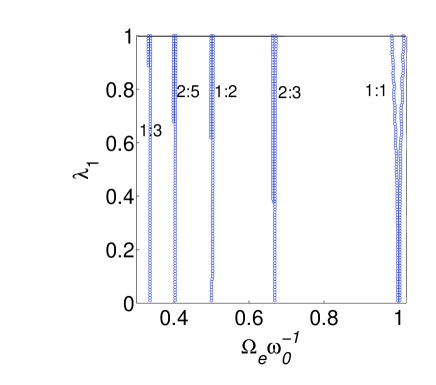
Figure 1: Arnol’d tongues: stability diagram for the parameter space defined by the amplitude $\lambda_{1}$ and frequency ratio $\Omega_{e}\omega_{0}^{-1}$. The boundaries that separate stable limit cycles from unstable and quasiperiodic solutions are shown. Frequency ratios of entrained limit cycle solutions inside each stability region are indicated. Parameters: $\epsilon=-0.2,~{}\nu=0.2,\xi=0.3125,B=1,\omega=1,M=1,k=0.36$. Original unperturbed limit cycle frequency: $\omega_{0}=0.7439$.

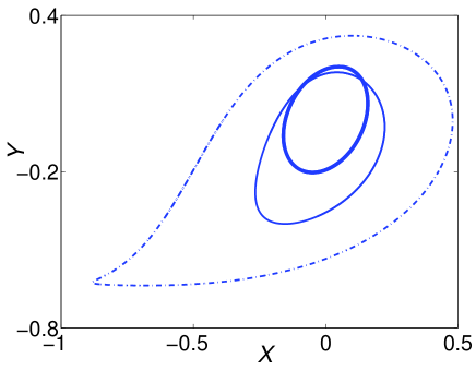
Figure 2: Examples of limit cycle solutions. Thick line shows the original limit cycle for $K(\lambda_{1},t)=k$ in system (4)-(6). Two other limit cycle solutions are calculated for the system (4)-(6) with non–zero amplitude of driving $\lambda_{1}=0.5~{}k$ (thin line), and with $\lambda_{1}=k$ (dash–dotted line). External frequency $\Omega_{e}=\omega_{0}=0.7439$ and the stiffness coefficient $k=0.36$.

III Effect of periodic modulation of stiffness

In this section, we discuss the effect of a non–additive periodic excitation on lock–in solutions stability in the system of self–oscillators coupled to an inertial load. The excitation is taken in the form of periodic modulation of the inertial oscillator stiffness coefficient. First we define a set of equations of motion and then proceed to examining the system stability domains. We study the amplitude dependence for frequencies of excitation near to the one–to–one resonance. Let us introduce a parametric modulation in the stiffness $k$ of the inertial oscillator (3) by using a periodic term $q(\lambda_{1},t)=\lambda_{1}\cos\Omega_{e}t$ with frequency $\Omega_{e}$ and amplitude $\lambda_{1}$. Then the expression for the force is:

$$F=-M\sum_{i=1}^{N}\mathrm{Re}(\ddot{z}_{i}+K(\lambda_{1},t)z_{i}+\nu\dot{z}_{i})$$ (5)

where $K(\lambda_{1},t)=k+q(\lambda_{1},t)$ is the time–dependent stiffness coefficient. In our treatment we include the case of a strong magnitude of driving by taking $\lambda_{1}/k\leq 1$. Upon differentiating both side of Eq. (4) and substituting the expression for $\ddot{z}_{i}$ from (5) the differential equation for the force yields:

$$\dot{F}=-\frac{\xi F}{NM}+\frac{\xi}{N}\sum_{i=1}^{N}\mathrm{Re}\bigg{\{}\frac{d\left(B|z_{i}|^{2}z_{i}+\mathrm{i}\omega z_{i}\right)}{dt}$$

$$-(\epsilon+\nu)\dot{z}_{i}-K(\lambda_{1},t)z_{i}\bigg{\}},$$ (6)

Together with Eq. (4) we now obtain a complete set of differential equations for $N+1$ variables. The displacement $x_{N+1}$ of the inertial oscillator is determined from the geometrical constraint (2). We expect that the stability behavior in system (4)-(6) is largely determined by a new type of coupling. As a consequence of the coupling the motion of every self–oscillatory element is affected by a common force. This force is explicitly dependent on time as well as on the oscillators displacement, velocity and acceleration.

III.1 Entrainment for an initially synchronized regime

Let us first discuss the entrainment behavior for initially homogeneous solutions: all the oscillators in ensemble are moving in phase and with the same frequency of oscillations. The linear stability analysis of the time–independent system in Ref. vilfan2003 provides a detailed phase diagram with the regions of stable globally synchronized solutions. Indeed, for the parameters space corresponding to $\epsilon<0$ and $\Omega_{0}<\Omega_{c}$ there exists a large set of stable synchronized solutions of Eqs. (4)-(6) for $\lambda_{1}=0$. When the synchronized state is stable it suffices to reduce systems description to the case of $N=1$ oscillator coupled with inertial load. However, when the parametric modulation is introduced in the model the stability problems for the system of $N=1$ and $N>1$ oscillators in the chain are no longer equivalent. The applied periodic excitation can change the stability of the synchronous solution for $N>1$. Thefore, the system can be driven to a new asymptoticcally inhomogeneous state. In our work we do not analyze the stability of synchronized solutions for the entire parameter space. Instead, we consider entrainment behavior of the synchronized state for a particular choice of parameters: $\epsilon=-0.2$ and $\Omega_{0}=0.6$. We integrate numerically the time-dependent system (4)-(6) with $N=1$ and $N=100$ oscillators. It follows that the observed entrainment behavior for the low–$(N=1)$ and high–dimensional $(N>1)$ cases matches well for the choice of parameters given above. Therefore, in order to simplify our analytical derivations and to speed up numerical procedure we reduce dynamical description of the system to the low–dimensional case. In the following paragraphs we discuss entrainment behavior for $N=1$ oscillator coupled with a mass load. For initial conditions we chose arbitrary small displacement $x_{1}=\mathrm{z_{1}}$. Results of numerical simulation are given in Fig. (1). We show stability domains in the parameter space defined by the amplitude of driving $\lambda_{1}$ and the ratio between external frequency $\Omega_{e}$ and the original limit cycle frequency $\omega_{0}$. Here the stability regions with lock–in solutions are separated from the regions of quasiperiodic and unstable solutions by defined boundaries. Inside each stability region the lock–in solution has rational frequencies ratio $m:n$. Note that the width of entrainment regions shortens as one proceeds from the $1:1$ resonance to the lower frequency ratios. Several limit cycle solutions are presented in Fig. (2) for the $1:1$ resonance and for different amplitudes $\lambda_{1}$.

III.2 Amplitude–frequency response

In this section we present numerical and analytical results on the amplitude–frequency dependence for the system (4)-(6). We use numerical analysis of fundamental frequencies laskar1992 to determine the amplitude of quasiperiodic and periodic solutions of the system (4)-(6) for the frequencies close to the one–to–one stimulation. For solutions $x=\mathrm{Re}z_{1}$ and $y=\mathrm{Im}z_{1}$ of (4)-(6) we obtain a quasiperiodic approximation near the vicinity of the original limit cycle solution of Eqs. (4)-(6) for $\lambda_{1}=0$. By using the substitution of solutions $x(t)$ and $y(t)$ with their zero time–averaged equivalents: $x(t)\rightarrow x(t)-\bar{x}$ and $y(t)\rightarrow y(t)-\bar{y}$ we write down the quasiperiodic expansions for the new $x(t)$ and $y(t)$:

$$x(t)=\sum_{q}c_{q}e^{\mathrm{i}\gamma_{q}t},~{}\quad~{}y(t)=\sum_{q}d_{q}e^{\mathrm{i}\gamma_{q}t},$$ (7)

where ${\gamma_{q}}$ is a set of time–independent frequencies. We assume that in the above expression the amplitudes ${c_{q}}$ and ${d_{q}}$ do not dependent on time. In the above expressions the terms are collected according to decreasing order of magnitude. To begin our numerical procedure we introduce a set of new coefficients $\tilde{c}_{n}$ and $\tilde{d}_{n}$ that are expressed from the following integrals laskar1992 :

$$\tilde{c}_{n} = \frac{1}{2T}\int_{-T}^{T}x(t)e^{-\mathrm{i}n(\pi/T)t}\chi(t)dt,$$ (8a)

$$\tilde{d}_{n} = \frac{1}{2T}\int_{-T}^{T}y(t)e^{-\mathrm{i}n(\pi/T)t}\chi(t)dt,$$ (8b)

where $\chi(t)=1+\cos\pi t/T$ is the Hanning window. The interval of time $100\pi\leq T\leq 300\pi$ is the integration time for every systems trajectory. Next, two sequences of coefficients ${c_{q}}$, and ${d_{q}}$ are produced by rearranging $\bar{c}_{n}$ and $\bar{d}_{n}$ according to the decreasing order of magnitude. In the expansions  (7) we only retain the first two terms that produce reasonably accurate approximation to the solutions $x(t)$ and $y(t)$. We calculate the first four largest coefficients of the series ${c_{q}}$ and ${d_{q}}$ as follows:

$$c_{1,-1}=\max\{{\tilde{c}_{1,-1},\tilde{c}_{2,-2},\ldots\}},$$ (9a)

$$d_{1,-1}=\max\{{\tilde{d}_{1,-1},\tilde{d}_{2,-2},\ldots\}},$$ (9b)

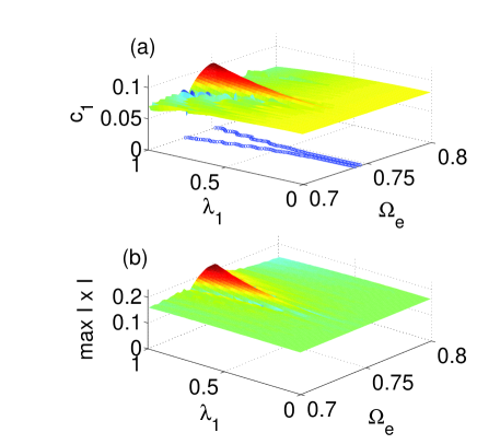
Figure 3: Amplitude–frequency response surface is shown on the $(\Omega_{e},\lambda_{1})$ plane. (a) Numerically calculated amplitude $c_{1}$ of the leading frequency component of the limit cycle in Eq. (5) near to the $1:1$ resonance for the driven system (4)-(6). Stability boundaries of the $1:1$ Arnol’d tongue are shown on the $(\Omega_{e},\lambda_{1})$ plane. (b) Numerically estimated maximum of the limit cycle solution for (4)-(6) with $\max|x|=\max_{{200\pi\leqslant t\leqslant 300\pi}}|x(t)-\bar{x}|$ for different amplitudes $\lambda_{1}$ and frequencies $\Omega_{e}$ of external driving. Parameters are: $\epsilon=-0.2,\nu=0.2,k=0.36,M=1,\xi=0.3125$.

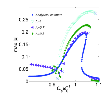
Figure 4: Amplitude–frequency response curves obtained at a fixed amplitude of $\Lambda=\lambda_{1}/k=[0.7,0.8,1]$ from Fig. (3). Analytical amplitude–frequency dependence $\Gamma_{\tilde{\lambda}_{1}}(\Omega_{e})$ is displayed (small circles) (see appendix for derivation). Here $\Omega_{e}\omega_{0}^{-1}=\Omega\Omega_{0}^{-1}(1-\Delta)$, where $\Delta=0.07\Omega^{-1}$ is the frequency mismatch. Parameters are given as in the Appendix. Numerically evaluated stability boundaries are shown (crosses) for all three values of $\Lambda$. Parameters for the analytical amplitude–frequency dependence: $\epsilon=-0.2,\nu=0.2,M=1,\omega=1,\xi=0.3125,\Omega_{0}=0.7861,\lambda_{1}=M\Omega_{0}^{2}$

Figure (3a) illustrates the parametric dependence of the largest coefficient $c_{1}$ in the expansion (9a) on the amplitude $\lambda_{1}$ and the frequency $\Omega_{e}$. Numerical responses are obtained by taking initial conditions for $x(t)$ and $y(t)$ to be randomly distributed in the vicinity of unperturbed limit cycle for Eqs. (4)-(6). For comparison we also calculated the maximum of the numerical solution over the same time interval $T$. Figure (3b) shows numerical results for the maximum of the amplitude $x(t)$:  $\max|x|=\max_{T}|x(t)|$. In the plane $(\Omega_{e},\lambda_{1})$ stability boundaries for the $1:1$ resonance are indicated. The results from two plots are consistent except for the regions near to the stability borders. The amplitude–frequency response is a surface that is smooth inside the borders of stability region and shows discontinuities outside near to the borders of Arnold tongue. Apparently, the discontinuities are due to the emergence of instabilities. Because of the instabilities, the leading frequency components that are defined from the quasiperiodic approximation (7) in this case might be distinctly different. Consequently, the numerical procedure produces a set of amplitudes which are not smoothly dependent on the external frequency $\Omega_{e}$.

We compare numerically estimated amplitude–frequency responses with the results obtained by using quasiperiodic approximation (see Appendix). In Fig. (4) three numerically calculated amplitude–frequency curves are displayed for different values of the amplitude $\Lambda=\lambda_{1}/k$. To compare these results with the analytical calculations, we display the amplitude–frequency curve $\Gamma_{\tilde{\lambda}_{1}}(\Omega_{e})$ obtained from the quasiperiodic approximation of limit cycle solution $(x(t),y(t))$ (see Eq. (19) in the Appendix). It is apparent, that for a given choice of parameters the curves from numerical and analytical calculations follow similar nonlinear response behavior inside the stability region (stability boundary is marked by crosses).

III.3 Entrainment for anti- and asynchronous regimes

In this section we illustrate results of numerical analysis for the periodic forcing of initially spatially inhomogeneous states. The existence and stability of these states for the autonomous system ($\lambda_{1}=0$) is controlled by the choice of a mass of inertial oscillator and parameter $\epsilon$. For the time–dependent system it is expected that under the influence of a strong driving these states might become unstable and converge to a new asymptotic state. In the limit of a large excitation it can produce significant changes on the regions of stability of existing spatiotemporal regimes. We demonstrate that, meanwhile some collective regimes do not survive new spatially homogeneous states become asymptotically stable. Here we show which conditions on the frequency and the amplitude of external driving have to be satisfied in order for the resulting spatial state to be stable and homogeneous.

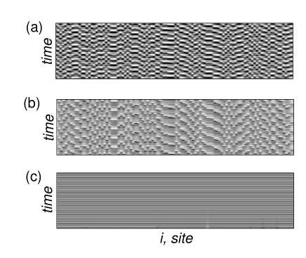
Figure 5: Space–time diagrams of intensity of oscillations $|z_{i}|$ for the $i$th element. (a) Asynchronous state for time–independent system  (4)-(6) ($\lambda_{1}=0$). (b) Asynchronous state for the time–dependent system (4)-(6) ($\lambda_{1}=k$).The frequency of driving $\Omega_{e}=\omega_{0}=0.85$. .(c) Synchronized behavior is obtained with the parametric forcing of an initially asynchronous state of system (10)-(11) ($\lambda_{2}=0.5\omega,\Omega_{e}=0.85$). Parameters for (a),(b) and (c): $\Omega_{0}=0.85,\epsilon=0.5,k=M\Omega_{0}^{2},M=1,\omega=1,\xi/N=0.3125,N=100$.

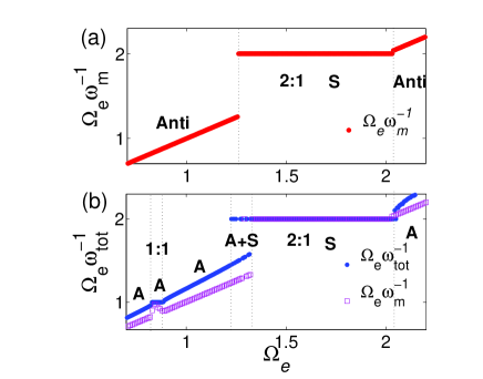
Figure 6: Frequency ratio curves for the antisynchronous (Anti) (asynchronous (A)) state of a chain of $N=100$ oscillators. (a) Ratio between external frequency $\Omega_{e}$ and the average oscillator frequency $\omega_{m}=1/N\sum_{i}^{N}\omega_{i}$ is plotted versus external frequency for an initially antisynchronous state of the system (4)-(6).(b) Frequency curves are plotted for an initially asynchronous state of the system  (4)-(6). Shown are two frequency ratio curves: $\Omega_{e}\omega_{m}^{-1}$ versus $\Omega_{e}$ (squares) and $\Omega_{e}\omega_{tot}^{-1}$ versus $\Omega_{e}$ (dots), where $\omega_{tot}$ is the frequency of the total extension $x_{tot}$ of a chain of oscillators. Parameters: $\epsilon=0.1$ for antisynchronous state, ($\epsilon=0.5$) for asynchronous state, $\Omega_{0}=0.85,k=M\Omega_{0}^{2},M=1,\omega=1,\xi/N=0.3125,\nu=0.2$ and $\lambda_{1}=k$ for both (a) and (b). The regions of stable synchronized states are indicated by (S).

In the literature studies of collective dynamics of chains of coupled oscillators are often reduced to their phase dynamics studies daido1996 ; pikovsky2001 . Our system is different from these cases because the amplitude of external force $F$ strongly depends on the state of the $i$th oscillator, and therefore, on the collective dynamics in an ensemble. It is not sufficient to confine the investigation only to a phase dynamics study, like in the cases of weakly coupled oscillators ermentrout1991 . It should be pointed out, that in the limit of a strong excitation the effect on amplitude variation of each individual oscillator has to be taken into account. Namely, for a large relative modulation $\lambda_{1}/k\sim 1$ not only the individual oscillator frequency is affected but also the amplitudes.

First, we proceed by considering the spatiotemporal state of the system  (4)-(6) with and without external parametric excitation. The time evolution of $N=100$ self–oscillators from an initially inhomogeneous collective state is followed by plotting space–time diagrams. These diagrams display a dynamical collective state of the system. In order to do so, we integrate $2N+1$ equations. The initial conditions are prepared by adding random perturbations to the initial zero state. Figure (5) shows the space–time diagram of the amplitude of $i$th oscillator $|z_{i}|$ on the $(i,t)$ plane for $N=50$ oscillators. The oscillator number is shown in abscissa and time $t$ in ordinate. Figure (5a) displays the time evolution of an asynchronous state from the initial time $t=0$ to the final time $t=300\pi$ in the absence of external periodic driving. A closer look reveals that the elements in the half of the ensemble ($i=1,\ldots 50$) are grouped in small clusters of oscillators. Each group consists of elements that are phase shifted with respect to the neighboring elements of the same group. As the external stimulation turned on the state in Fig. (5a) evolves to a new asynchronous state shown in the panel (b) of the same figure. It presents the time–evolution of an inhomogeneous unstable state for $N=50$ oscillators and the frequency of excitation $\Omega_{e}=0.85$. It can be easily seen that the distribution of groups of oscillators remains the same as in Fig. (5a) but the average self–oscillator frequency is shifted towards the stimulation frequency $\Omega_{e}$. The state is not stable, and is sensitive to variations of initial distributions of the positions and the velocities of the oscillators. In fact, the value of numerically estimated Lyapunov exponent is positive in this case. Such regimes are found for the CGLE with an additive periodic forcing chate1999 . These ”turbulent synchronized states” arise in the situation when the forcing is weak and its frequency is chosen nearly the same as a natural oscillation frequency chate1999 . In this case the dynamical state is characterized by the average frequency of collective excited oscillations being equal to external frequency and its numerical Lyapunov exponent being greater than zero.

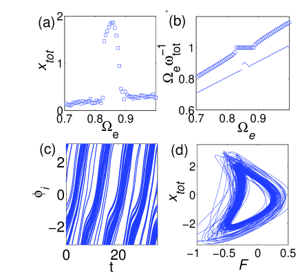
Figure 7: Asynchronous state of oscillators near the $1:1$ resonant driving region from Fig. (6b). (a) Amplitude of total extension $x_{tot}=\sum_{i=1}^{N}x_{i}$ of a chain of $N=100$ oscillators versus external frequency $\Omega_{e}$. (b) Two frequency ratios versus external frequency are displayed: $\Omega_{e}\omega_{m}^{-1}$ (dots) and $\Omega_{e}\omega_{tot}^{-1}$ (circles). $\omega_{m}$ is the average frequency of oscillators in a chain, $\omega_{tot}$ in the frequency of total extension. (c) Phase $\phi_{i}=\arg(z_{i})$ of $N=100$ active elements as a function of time for asynchronous state solution for $\Omega_{e}=0.85$. (d) Example of quasiperiodic solution plotted for $x_{tot}$ versus force $F$. $\Omega_{e}=0.85$ for (c) and (d).

Finally, a perfectly synchronized solution is displayed in Fig. (5c). Unlike in the previous two plots, here after a short transient time the ensemble is organized into coherent structure with all the individual elements moving in phase and with the frequency $\Omega_{e}$. To produce this plot another type of stimulation is used that will be discussed in the following sections.

We will specify the transitions that occur in the system for various stimulation frequencies by plotting the frequency ratio curves versus the stimulation frequency. Figure (6) displays two cases for distinct parameter choices. Frequency ratio curves for an initially antisynchronous state and for an initially asynchronous state are shown in Fig. (6) (a) and (b). Let us first examine the changes in dynamical behavior if we chose the parameters from the domain that corresponds to an antisynchronous oscillatory regime stable for the time–independent system. This can be easily done by defining the bifurcation parameter $\epsilon=0.1$ and by taking the frequency of the inertial oscillator $\Omega_{0}=0.85$ vilfan2003 . We plot in Fig. (6a) the frequency ratio curves $\Omega_{e}\omega_{m}^{-1}$ versus $\Omega_{e}$. Several distinct regions that correspond to different collective dynamical states exist. The system remains in the antisynchronous state for an interval $\Omega_{e}\in[0.2;1.2]$. For higher frequencies $\Omega_{e}\in[1.22;2.03]$ the solution is driven into the synchronized $2:1$ state. This synchronized state is characterized by all the oscillatory elements moving in–phase and with the same frequency. Upon increasing the excitation frequency $\Omega_{e}\geq 2.03$ the system undergoes a transition to an antisynchronous behavior. We examine now the transitions in frequency that occur for an initially asynchronous state. By adjusting the bifurcation parameter to $\epsilon=0.5$ one insures the existence of an asymptotically stable asynchronous state of the unperturbed system ($\lambda_{1}=0$)  (4)-(6). The frequency of the inertial oscillator is chosen to be the same as defined above. We present results of numerically calculated frequency ratios in Fig. (6b). Two curves are presented: the frequency ratio $\Omega_{e}\omega_{tot}^{-1}$ between external driving frequency and the frequency of the total extension $x_{tot}=\sum_{i=1}^{N}x_{i}$ versus $\Omega_{e}$ (squares) and the frequency ratio $\Omega_{e}\omega_{m}^{-1}$ versus $\Omega_{e}$ (dotted curve), where $\omega_{m}$ is the spatially averaged frequency. One can observe that transitions from one collective state to the other are controlled by changing the frequency $\Omega_{e}$. In particular, there exists a $1:1$ plateau that indicates the region of quasiperiodic asynchronous solutions. There are several transient regimes calculated for different values of the external driving $\Omega_{e}$: asynchronous states for $\Omega_{e}=[0.2;1.2]$, the region of coexistence of synchronous and

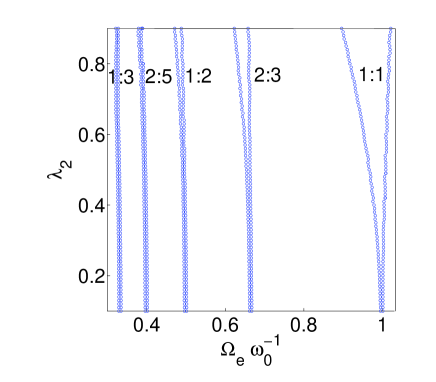
Figure 8: Arnol’d tongues: stability diagram for the parameter space defined by amplitude $\lambda_{2}$ of external driving and frequency ratio $\Omega_{e}\omega_{0}^{-1}$. The boundaries separating stable limit cycles from unstable and quasiperiodic solutions are shown. The frequency ratios of entrained limit cycle solutions inside each region are indicated. Parameters are: $\epsilon=-0.2,\nu=0.2,\xi=0.3125,B=1,\omega=1,M=1,k=0.4$. Frequency of an unperturbed limit cycle solution $\omega_{0}=0.6337$.

asynchronous states for $\Omega_{e}=[1.2;1.35]$ at the border with the $2:1$ resonance. A large set of synchronized solutions emerges for the $2:1$ ratio when all the oscillatory elements are phase locked to the $2:1$ frequency ratio regime. Note, that although for the initially antisynchronous state the one–to–one stable entrainment regime is not present (see Fig. (6a)) this regime exist for the initially asynchronous state. For a detailed view on this regime we refer to Fig. (7) which shows a magnification of the $1:1$ plateau. Numerically calculated nonlinear amplitude response (see Fig. (7a)) for a total chain extension $x_{tot}$ and the $1:1$ plateau in Fig. (7b) are magnified for ranges of frequencies $\Omega_{e}$ that lie close to the $1:1$ resonance. In Fig. (7c) the evolution of oscillator phases $\phi_{i}=arg(z_{i})$ is plotted for $N=50$. An example of quasiperiodic solution for $1:1$ resonance is presented in Fig. (7d). Here, the oscillation of tension force $F$ is displayed versus the total chain extension $x_{tot}$.

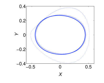
Figure 9: Limit cycle solutions for the system (10)-(11). Thick line shows the original limit cycle for the autonomous system (10)-(11) ($\lambda_{2}=0$). Two limit cycle solutions (thin and dotted curves) are displayed for the system (10)-(11) with $\lambda_{2}=\omega$ and external frequency $\Omega_{e}=0.6337$ (dotted line), and with $\lambda_{2}=0.1\omega$ (thin line). Parameters are the same as in Fig. (8).

Our results suggests, that the final collective behavior depends on the choice of initial collective state of the system. Indeed, as we have seen in Fig. (6) the same stimulation frequency results in two distinct final states. One interesting detail, that the stability diagrams indicate the largest set of the $2:1$ entrained solutions. The emergence of these solutions is due to the presence of the multiplicative periodic modulation that produces the $2:1$ harmonic terms in the system equations.

IV System with parametric modulation of frequency of limit cycle oscillators

In this section we discuss the synchronization dynamics for the system of self–oscillators with a parametric modulation of the frequency of self–oscillatory element. We modify a set of equations  (4)–(6) by setting $\lambda_{1}=0$ and introducing a periodic term $g(\lambda_{2},t)=\lambda_{2}\cos\Omega_{e}t$ with the frequency $\Omega_{e}$ and the amplitude $\lambda_{2}$. The resulting equation for the $i$th oscillator can be written as follows:

$$\dot{z}_{i}=(\mathrm{i}\varrho(\lambda_{2},t)+\epsilon)z_{i}-B|z_{i}|^{2}z_{i}+F\xi^{-1},$$ (10)

Where $\varrho(\lambda_{2},t)=\omega+g(\lambda_{2},t)$ is the time–dependent frequency modulation term. Consequently, the equation for the force yields:

$$\dot{F}=-\frac{\xi F}{NM}+\frac{\xi}{N}\sum_{i=1}^{N}\mathrm{Re}\bigg{\{}\frac{d\left(B|z_{i}|^{2}z_{i}+\mathrm{i}\varrho(\lambda_{2},t)z_{i}\right)}{dt}$$

$$-(\epsilon+\nu)\dot{z}_{i}-\Omega_{0}^{2}z_{i}\bigg{\}},$$ (11)

IV.1 Stability diagram for the synchronized state

Analogously to the previous section where we first discussed the entrainment behavior for the low–dimensional system, here we study first the case of $N=1$ oscillator. By choosing $\epsilon<0$ and the linear oscillator frequency $\Omega_{0}$ below the critical value $\Omega_{c}$ we assert that the stable globally synchronized state exist for the autonomous system (10)-(11) ($\lambda_{2}=0$). We intergate the set of equations (10)-(11) with initial conditions picked randomly near to the trivial solution. We carry out numerical stability for a non–zero parametric modulation $g(\lambda_{2},t)$. In order to reach the limit of a strong excitation we define the amplitude of the modulating term to be comparable with the amplitude of a self–oscillating element frequency $\lambda_{2}/\omega\leq 1$. Figure (8) shows Arnol’d tongues calculated numerically. Inside the stability regions the frequency ratios are identified for each resonance. Examples of the limit cycle solutions for the unperturbed system ($\lambda_{2}=0$) and for the perturbed system with $\lambda_{2}\omega^{-1}=0.1$ and $\lambda_{2}\omega^{-1}=1$ are shown in Fig. (9).

IV.2 Amplitude–frequency response

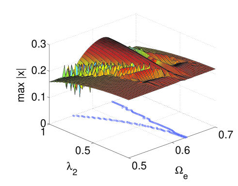
Figure 10: Amplitude–frequency response surface. Numerically calculated maximum of solution $x(t)$: $\max|x|$ for the system (10)-(11). The stability boundary of $1:1$ entrainment region is shown on the $(\Omega_{e},\lambda_{2})$ plane. Parameters: $\epsilon=-0.2,\nu=0.2,k=0.4,M=1,\xi=0.3125$. The frequency of an unperturbed limit cycle is $\omega_{0}=0.6337$.

In Fig. (10) the amplitude–response surface is presented from numerical calculations of the maximum of solution $x(t)$ for the system (10)-(11). The maximum is estimated over the entire interval of integration and obtained from the zero–averaged solution $\max|x|=\max_{200\pi\leq t\leq 300\pi}|x(t)-\bar{x}|$. The borders of stability region are displayed on the $(\Omega_{e},\lambda_{2})$ plane. The response is smooth inside the one–to–one entrainment stability zone. It strongly shows nonlinear features for large amplitude of the periodic driving: $\lambda_{2}\leq\omega$.

IV.3 Entrainment for inhomogeneous states

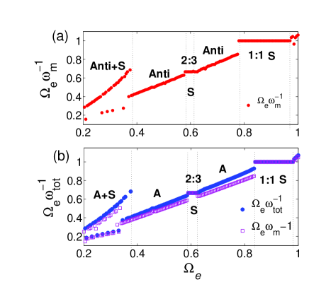
Figure 11: Frequency ratio curves versus external frequency $\Omega_{e}$ calculated from the Eqs. (10) and  (11). Parameters: $(\epsilon=0.1)$ for antisynchronous state in (a), $(\epsilon=0.5)$ for asynchronous state in (b), $\Omega_{0}=0.85$ and $\lambda_{2}=0.5\omega$.

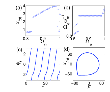
Figure 12: Synchronized state of oscillators inside the $1:1$ resonant region in Fig. (11b). External driving frequency $\Omega_{e}=0.85$ for (c) and (d).

Now we turn to the case of entrainment behavior for inhomogeneous states. We compute frequency ratio curves for initially inhomogeneous states of a chain of $N=100$. The stimulation frequency is chosen within the interval $[0.2;1]$ in order to include the $1:1$ resonance and the lower ratio resonances. The results are reproduced in Fig. (11) for an initially antisynchronous state (a) and for an initially asynchronous state (b). In both cases, one can distinguish two well–pronounced extended plateaus at the $2:3$ and the $1:1$ resonances. The plateaus indicate the perfectly entrained solutions with all the oscillatory units moving in phase and with the frequency of $\Omega_{e}$. The remaining solutions that does not belong to the entrainment regions are inhomogeneous states. They display qualitatively different spacial dynamics. Each state is characterized by the individual oscillators forming macroscopic clusters. The motion of the individual units in a cluster is quasiperiodic. One can observe a region of multistability for low values of $\Omega_{e}$. Stable coexisting homogeneous and inhomogeneous states can be found inside this region. In the following figure (12) the magnification on the one–to–one synchronized state is displayed. This state is obtain from an initially randomly distributed phases of individual elements in the chain. Th amplitude of modulation is $\lambda_{2}=0.5\omega$ and the external frequency $\Omega_{e}=0.85$. The space–time plot of the synchronized state ca be also viewed in Fig. (5c). After a short transient all the oscillators begin to move in phase and with frequency equal to $\Omega_{e}$. For the synchronized state shown in Fig. (12) the frequency of the total extension $x_{tot}$ and the frequencies of self–oscillatory elements math the stimulation frequency $\Omega_{e}$. In Fig. (12a) and (b) the amplitude response and the frequency ratio are plotted versus $\Omega_{e}$. The periodic orbit in the space of variables $F$ and $x_{tot}$ is also shown.

V Discussion

In this work we study entrainment behavior in an ensemble of identical limit cycle oscillators coupled via geometrical constraint and via a common force to an inertial linear oscillator. The external force due to a mass–spring load provides a global coupling: it acts on each element of the ensemble. We consider an external parametric modulation as a time–dependent force acting in addition to the applied force due to a mass load The collective dynamics of oscillatory elements undergoes several transitions between different inhomogeneous states. Such transitions are ruled by the frequency and the type of parametric modulations introduced in the model. Based on our description we find families of stable oscillatory synchronized solutions corresponding to the resonant external stimulation of the system. We discuss an influence of two types of parametric excitations: periodic modulation of the stiffness of the inertial load and modulation of the frequency of self–oscillatory element. In particular, we demonstrate that for the spatially synchronized state the second type of excitation leads to larger stability domains than the first type of excitation. Furthermore, we show that with the appropriate parametric modulation introduced an initially inhomogeneous state of the system is driven into the $1:1$ synchronized state with the frequency of collective oscillations equal to the external frequency. Our conclusion is that such globally synchronized behavior can not be achieved from an initially inhomogeneous state by the periodic modulation of the stiffness coefficient. Instead a new type of dynamical state is observed. The emergent spatially inhomogeneous behavior can be described as a partially synchronized state: while every individual element moves with a frequency higher than the frequency of the total chain extension, the sum of displacements of all the elements oscillate at a frequency equal to the external stimulation frequency.

The amplitude–frequency characteristic shows a typical nonlinear response behavior with a fold in the parameter space defined by the driving frequency and the amplitude of the response. Our numerical results show a good agreement with the quasiperiodic approximation inside the one–to–one stable entrainment zone.

The phenomena discussed here have relevance and applications in nature and laboratories. In particular, the autonomous model and its time–dependent analogue provide a phenomenological approach to model oscillatory dynamics of an active muscle fiber. Experimental in vitro observations on skinned muscle fiber show evidence of different oscillatory regimes generated by spontaneous contractions of muscle elementary units, sarcomeres yasuda1996 . Depending on the conditions of the experiment, oscillatory contractions can undergo a synchronized activity yasuda1996 or a spatially inhomogeneous (asynchronous or antisynchronous) activity okamura1988 ; fukuda1996 . In experiments the signalling between adjacent sarcomeres is chemically regulated. The state of activation of one sarcomere is affected by the state of the adjacent sarcomere yasuda1996 . Our current model does not consider the effect of coupling between adjacent sites in the chain of elements. In the future we plan to include local coupling between elements and to consider its effect on spatiotemporal dynamics. Detailed study of the corresponding regimes of spatiotemporal behavior is left to future work.

Experimental work and results from theoretical analysis of our phenomenological model promise new interesting insights into collective behavior of oscillations in isolated fibrillar muscle. Periodic modulation of the model parameters considered here might serve as an appropriate setting for modeling active muscle contractions under a specially designed external mechanical and chemical stimulation.

VI Appendix

In the appendix, we discuss a quasiperiodic approximation bogoliubov1961 used for derivation of the nonlinear amplitude–frequency dependence. The derivation is carried out for the first type of parametric modulation discussed in the paper. It can be seen from Fig. (2) that the original unperturbed limit cycle is close to the ellipse centered at zero. Solutions for a non–zero small perturbation $\lambda_{1}\ll k$ are nearly close to the disturbed elliptical form with their centers shifted away from zero. These observations lead us to seek the solutions expansion in form of a finite series of harmonic terms, where the largest contribution terms represent solution for an ellipse. The system  (4)-(6) can be rewritten in a real form after introducing $x=\mathrm{Re}(z)$ and $y=\mathrm{Im}(z)$ variables with $x$ a displacement of the oscillator and $y$ a time–dependent variable nonlinearly coupled to $x$:

$$M/\xi\ddot{x} = -\left(1+M\nu/\xi\right)\dot{x}-K(\lambda_{1},t)/\xi x$$ (12a)

$$-\omega y+\epsilon x-B(x^{2}+y^{2})x,$$

$$\dot{y} = \omega x+\epsilon y-B(x^{2}+y^{2})y,$$ (12b)

For the non–autonomous system (12) a limit cycle solution can be written in the quasiperiodic form tomita1977 :

$$x = a_{1}\cos~{}\Omega t+b_{1}\sin~{}\Omega t+a_{0}+\ldots,$$ (13a)

$$y = b_{2}\sin~{}\Omega t+a_{2}\cos~{}\Omega t+a_{g}+\ldots.$$ (13b)

Where $\Omega$ is the frequency of a new limit cycle for the time–dependent system (12). The amplitude coefficients in the expansion  (13) depend on the size of the original unperturbed limit cycle solution and are ordered according to the powers of $\epsilon$: $a_{1},b_{2},a_{g}$ are of order $O(\epsilon^{1/2})$,  $b_{1},a_{2}$ are of order $O(\epsilon)$ and $a_{0}=O(\epsilon^{3/2})$. If the driving frequency $\Omega_{e}$ is near to the frequency $\omega_{0}$ of the limit cycle solution for the unperturbed system $(\lambda_{1}=0)$ in (4)-(6) a reasonable approximation for the $1:1$ lock–in solution can be made by retaining only terms to the accuracy of $O(\epsilon^{2})$ in Eqs. (13). We would not consider the terms of order equal to $O(\epsilon^{2})$ in the approximation presented here. Coefficients of the expansion (13) can be expressed via coefficients in (7) as follows:

$$a_{1} = \frac{c_{1}+c_{-1}}{2},~{}b_{1}=\frac{\mathrm{i}(c_{-1}-c_{1})}{2},~{}a_{0}=\bar{x},$$ (14a)

$$a_{2} = \frac{d_{1}+d_{-1}}{2},~{}b_{2}=\frac{\mathrm{i}(d_{-1}-d_{1})}{2},~{}a_{g}=\bar{y}.$$ (14b)

We introduce a small parameter $\Delta=\Omega-\Omega_{e}=O(\epsilon^{2})$ to be a frequency mismatch between the external frequency and the resulting limit cycle frequency. Let us define a linear frequency:

$$\Omega_{0}=\omega/(1+M\nu/\xi)^{1/2}.$$

Consequently, one finds that the frequency ratio $\Omega_{e}\omega_{0}^{-1}$ can be expressed as follows:

$$\Omega_{e}\omega_{0}^{-1}\approx\Omega\Omega_{0}^{-1}(1-\Delta).$$

In the next step, we use the quasiperiodic approximation (13) to derive a final form of the amplitude–frequency response. We assume that the following expansion holds true: $k=k_{0}+\epsilon k_{1}$, with $k_{0}=M\Omega_{0}^{2}$. For the sake of simplicity, we introduce the rescaling of the parameters:

$$\tilde{m}\rightarrow M/\xi,\tilde{k}\rightarrow k/\xi,~{}\tilde{\lambda_{1}}\rightarrow\lambda_{1}/\xi.$$

Upon substituting the quasiperiodic form (13) into Eq. (5) and collecting various terms according to the order of harmonics we obtain a set of nonlinear equations:

$$\tilde{m}\ddot{a_{0}}= -(1+\tilde{m}\nu)\dot{a_{0}}+(\epsilon-\tilde{k})a_{0}$$ (15a)

$$-\omega a_{g}-\tilde{\lambda_{1}}a_{1}/2-g_{1}a_{0}$$

$$-a_{1}g_{2}-b_{1}g_{3},$$

$$\dot{a_{g}}= \epsilon a_{g}+\omega a_{0}-a_{g}g_{1}-a_{2}g_{2}$$ (15b)

$$-b_{2}g_{3},$$

$$\ddot{a_{1}}= -(1+\tilde{m}\nu)\dot{a_{1}}+\Omega^{2}\tilde{m}a_{1}$$ (15c)

$$-(1+\tilde{m}\nu)\Omega b_{1}+(\epsilon-\tilde{k})a_{1}-\omega a_{2}$$

$$-\tilde{\lambda_{1}}a_{0}-a_{1}g_{1}-2a_{0}g_{2}$$

$$-a_{1}g_{4}/4-b_{1}g_{5}/2,$$

$$\dot{a_{2}}= -\Omega b_{2}+\epsilon a_{2}+\omega a_{1}-2a_{g}g_{2}$$

$$-a_{2}g_{1}-a_{2}g_{4}/4-b_{2}g_{5}/2,$$

$$\dot{b_{2}}= \Omega a_{2}+\epsilon b_{2}+\omega b_{1}-2a_{g}g_{3}-b_{2}g_{1}$$ (15d)

$$-a_{2}g_{5}/2+b_{2}g_{4}/4,$$

$$\tilde{m}\ddot{b_{1}}= -(1+\tilde{m}\nu)\dot{b_{1}}+\tilde{m}\Omega^{2}b_{1}$$ (15e)

$$+(1+\tilde{m}\nu)\Omega a_{1}+(\epsilon-\tilde{k})b_{1}-\omega b_{2}$$

$$-2a_{0}g_{3}-a_{1}g_{5}/2-b_{1}g_{1}$$

$$-b_{1}g_{4}/4,$$

where $g_{1},g_{2},g_{3}$ are nonlinear functions of the coefficients in (13):

$$g_{1} = B\bigg{(}a_{0}^{2}+a_{g}^{2}+\frac{a_{1}^{2}}{2}+\frac{a_{2}^{2}}{2}+\frac{b_{2}^{2}}{2}+\frac{b_{1}^{2}}{2}\bigg{)},$$

$$g_{2} = B(a_{0}a_{1}+a_{g}a_{2}),$$

$$g_{3} = B(a_{0}b_{1}+a_{g}b_{2}),$$

$$g_{4} = B(a_{1}^{2}-b_{1}^{2}+a_{2}^{2}-b_{2}^{2}),$$

$$g_{5} = B(a_{1}b_{1}+a_{2}b_{2}).$$

We would not consider the terms of order $O(\epsilon^{3/2})$ in the approximation presented here. Let us make the assumption that for the entrained limit cycle solution (13) the coefficients in the expansion (13) are constant or vary slowly with time. Then one can neglect derivatives from the equations for the coefficients (15). By neglecting terms of order $O(\epsilon^{3/2})$ one can express the coefficients $a_{2},a_{g},b_{1}$ and $b_{2}$:

$$a_{g}=-\frac{\tilde{\lambda}_{1}}{2\omega}a_{1},$$ (17a)

$$a_{2}=-\frac{\omega}{\Omega}b_{1},~{}b_{2}=\frac{\omega}{\Omega}a_{1},$$ (17b)

$$b_{1}=\frac{(1+\tilde{m}\nu)\Omega-\omega^{2}/\Omega}{\tilde{m}(\Omega_{0}^{2}-\Omega^{2})}a_{1}.$$ (17c)

Let us use the substitution $\rho=a_{1}^{2}$. Our final goal is to obtain a family of amplitude–frequency curves:

$$\Gamma_{\tilde{\lambda}_{1}}(\Omega_{e}):\Omega_{e}\omega_{0}^{-1}\rightarrow\rho(\Omega\Omega_{0}^{-1}).$$

After substituting the expressions (17) for the coefficients into Eqs. (15) and eliminating terms of the order $O(\epsilon^{3/2})$ we write down the approximate amplitude–frequency relation:

$$a_{0}\tilde{\lambda}_{1}^{2}= \frac{B^{2}}{16}\bigg{[}\tilde{\lambda}_{1}^{2}+\left(3+\frac{\omega^{2}}{\Omega^{2}}\right)\left(1+\frac{1}{\tilde{m}^{2}}\frac{\omega^{4}}{\Omega_{0}^{4}\Omega^{2}}\right)\bigg{]}^{2}\rho^{3}-\frac{B}{2}\bigg{[}\left(\tilde{m}-\frac{\omega^{4}}{\tilde{m}\Omega_{0}^{4}\Omega^{2}}\right)(\Omega^{2}-\Omega_{0}^{2})+\epsilon\left(1-\tilde{k}_{1}\right)\bigg{]}\times$$ (19)

$$\bigg{(}3+\frac{\omega^{2}}{\Omega^{2}}\bigg{)}\Bigg{(}1+\frac{1}{\tilde{m}^{2}\Omega_{0}^{4}\Omega^{2}}\bigg{)}\rho^{2}+\bigg{[}\bigg{(}\tilde{m}^{2}+\bigg{(}\frac{\omega^{4}}{\tilde{m}\Omega_{0}^{6}}\bigg{)}^{2}\bigg{)}\left(\Omega^{2}-\Omega_{0}^{2}\right)^{2}-2\bigg{(}\frac{\omega^{2}}{\Omega}-(1+\tilde{m}\nu)\Omega\bigg{)}^{2}+2\epsilon(\tilde{k}_{1}-1)\times$$

$$\bigg{(}\tilde{m}-\frac{\omega^{4}}{\tilde{m}\Omega_{0}^{4}\Omega^{2}}\bigg{)}(\Omega_{0}^{2}-\Omega^{2})\bigg{]}\rho,$$

Finally, what remains to be done is to determine a set of parameters for calculating the relation (19). Let us define the parameters in order to compare with the numerical results: $\epsilon=-0.2,\nu=0.2,M=1,\omega=1,\xi=0.3125,\Omega_{0}=0.7861,\lambda_{1}=k_{0},a_{0}=0.01\lambda_{1}^{-2}$. We have used $\Delta=0.07~{}\Omega_{0}\Omega^{-1},~{}k_{1}=0.4\xi$ in order to obtain a reasonable fitting to the numerical amplitude–frequency response in Fig. (4).

VII Acknowlegements

The author thanks E. Nicola for many useful comments and suggestions regarding implementation of numerical code. The author is grateful to S. Ares for his comments on the manuscript. The author would like to acknowledge M. Zapotocky for helpful discussions. This research was partially funded by the VolkswagenStiftung Foundation and the Max-Planck-Gesellschaft.

References

- (1) L. Glass, A. Shrier, in L. Glass, P. Hunter, A. McCulloch,(Eds.),Theory of Heart,Spinger, New York,289 (1991)
- (2) C. Graves, L. Glass, D. Laporta, R. Meloche, A. Grassino, Am. J. Physiol.(Regulat. Integrat. Comp. Physiol. 19) 250 R902 (1986)
- (3) M. H. Dickinson, Current Biology 16 R309 (2006)
- (4) G. Nalbach, Proc. Göttingen Neurobiol. Conf. 16 131 (1988)
- (5) F. -O Lehmann, M. H. Dickinson, J. Exp. Biol. 200 1133 (1997)
- (6) A. Pikovsky, M. Rosenblum, J. Kurths, Synchronization: a Universal Concept in Nonlinear Science,Cambridge University Press, New York,(2001)
- (7) L. Glass, Nature 401 277 (2001)
- (8) H. D. Abarbanel, M. I. Rabinovich, Current Opinion in Neurobiology 11 423 2006
- (9) H. Chate, A. Pikovsky, O. Rudzick, Physica D 131 17 (1999)
- (10) G. V. Osipov, J. Kurths, C. Zhou, Synchronization in Oscillatory Networks, Springer-Verlag, Berlin Heidelberg, (2007)
- (11) V. S. Afraimovich, V. I. Nekorkin, G. V. Osipov, V. D. Shalfeev, Stability, Structures and Chaos in Nonlinear Synchronization Networks, World Scientific, Singapure, (1994)
- (12) S. Rüdiger, E. M. Nicola, J. Casademunt, L. Kramer, Phys. Rep. 447 73 (2007)
- (13) D. Battogtokh, A. Mikhailov, Physica D 90 84 (1996)
- (14) Y. Kuramoto, Chemical Oscillations, Waves and Turbulence, Springer-Verlag, Berlin,(1984)
- (15) P. Coullet, K. Emilsson, Physica D 61 119 (1992)
- (16) S. D. Drendel, N. P. Hors, V. A. Vasiliev, Dynamics of Cell Populations, Nizhny Novgorod University Press, Nizhny Novgorod, (1984)(in Russian)
- (17) T. E. Vadivasova, G. E. Strelkova, V. S. Anishchenko, Phys. Rev. E 63 036225 (2001)
- (18) H. Hakim, W.-J. Rappel, Phys. Rev. A 46 7347 (1992)
- (19) D. Topaj, A. Pikovsky, Physica D 170 118 (2002)
- (20) A. Vilfan, T. Duke, Phys. Rev. Lett. 91 114101 (2003)
- (21) K. Yasuda, Y. Shindo, S. Ishiwata, Biophys. J. 70 1823 (1996)
- (22) , J. Laskar, C. Froeschlé, A. Celletti, Physica D 56 253 (1992)
- (23) H. Daido H, Physica D 91 24 (1996)
- (24) G. B. Ermentrout, N. Kopell, J. Math. Biol. 29 195 (1991)
- (25) N. Fukuda, H. Fujita, T. Fujita and S. Ishiwata, Eur. J. Physiol. 433 1 (1996)
- (26) , N. Okamura, S. Ishiwata, J. Muscle Res.Cell Motil. 9 111 (1988)
- (27) , N. N. Bogoliubov, Y. A. Mitropolsky, Asymptotic Methods in the Theory of Nonlinear Oscillators, Gordon and Breach, New York,(1961)
- (28) K. Tomita, T. Kai, F. Hikami, Prog. Theor. Phys. 57 1159 (1997)