Polarized Emission of Sagittarius A*

Abstract

We explore the parameter space of the two temperature pseudo-Newtonian Keplerian accretion flow model for the millimeter and shorter wavelength emission from Sagittarius A*. A general relativistic ray-tracing code is used to treat the radiative transfer of polarized synchrotron emission from the flow. The synchrotron self-Comptonization and bremsstrahlung emission components are also included. It is shown that the model can readily account for the millimeter to sub-millimeter emission characteristics with an accretion rate of $\sim 6\times 10^{17}\mathrm{g}\cdot\mathrm{s}^{-1}$ and an inclination angle of $\sim 40^{\circ}$. However, the corresponding model predicted near-infrared and X-ray fluxes are more than one order of magnitude lower than the observed ‘quiescent’ state values. While the extended quiescent-state X-ray emission has been attributed to thermal emission from the large-scale accretion flow, the NIR emission and flares are likely dominated by emission regions either within the last stable orbit of a Schwarzschild black hole or associated with outflows. With the viscous parameter derived from numerical simulations, there is still a degeneracy between the electron heating rate and the magnetic parameter. A fully general relativistic treatment with the black hole spin incorporated will resolve these issues.

1 INTRODUCTION

Sagittarius (Sgr) A*, the compact radio source associated with the super-massive black hole at the Galactic center, is perhaps the best source for the study of physical processes near the event horizon of a black hole (Schödel et al., 2002; Ghez et al., 2005). Although its luminosity is relatively low, with the high resolution and sensitivity of modern instruments, the source has been routinely observed from radio to X-rays. It may also play a role in the production of TeV gamma-ray emission from the Galactic center region (Liu et al., 2006; Aharonian et al., 2006). The low luminosity also renders the source optically thin at millimeter and shorter wavelengths. One therefore can observe emission from the very inner region close to the black hole directly at these wavelengths.

Most of Sgr A* emission is released in the sub-millimeter band, where a strong linear polarization is observed. The flux density also varies with the variation amplitude and rate decreasing with the decrease of the observation frequency (Herrnstein et al., 2004). The variation timescale of sub-millimeter emission can be as short as a few hours, slightly longer than the dynamical time near the black hole. The source is highly variable at shorter wavelengths with the peak luminosity of some near infrared (NIR) and X-ray flares comparable to the sub-millimeter luminosity (Baganoff et al., 2001; Genzel et al., 2003) The variation timescale of these flares is consistent with events occurring within a few Schwarzschild radii of the black hole. And correlated flare activities in the X-ray, NIR, millimeter, and radio bands suggest outflows during some flares (Zhao et al., 2004; Yusef-Zadeh et al., 2007; Marrone et al., 2007; Eckart et al., 2008). The flares also contain rich temporal, spectral, and polarization information (Porquet, 2008; Falanga et al., 2008; Eckart et al., 2008). Detailed modelling of these emission characteristics is expected to probe the geometry near the black hole, processes of the general relativistic magnetohydrodynamics (GRMHD) (Gammie et al., 2003), and the kinetics of electron heating and acceleration in a magnetized relativistic plasma (Liu et al., 2004, 2007b).

Motivated by MHD simulations of radiatively inefficient accretion flows (Hawley & Balbus, 1991, 2002), we proposed a Keplerian accretion flow model for the time averaged millimeter and shorter wavelength emission from Sgr A* (Melia et al., 2000, 2001). The model plays important roles in constraining the time averaged properties of the plasma near the black hole (Yuan et al., 2003) for detailed GRMHD studies (Noble et al., 2007). It also treats the polarization characteristics quantitatively (Bromley et al., 2001). The model is later generalized to a two temperature accretion flow in a pseudo-Newtonian potential (Liu et al., 2007a, b). Huang et al. (2008) first carried out a self-consistent treatment of the transfer of polarized emission through the accretion flow and predicted distinct linear and circular polarization characteristics between the sub-millimeter and NIR band due to general relativistic light bending and birefringence effects. In this paper, we present the details of the calculations (§ 2), explore the model parameter space (§ 3), and discuss future developments (§ 4).

2 RADIATIVE TRANSFER OF SYNCHROTRON RADIATION

Although the importance of a self-consistent treatment of polarized radiative transfer through relativistic plasmas near black holes was recognized a while ago (Melrose, 1997), there are still significant uncertainties in the quantitative details (Shcherbakov, 2008). The thermal synchrotron emission and absorption coefficients have been derived independently by several authors (Legg & Westfold, 1968; Sazonov, 1969; Melrose, 1971), which in general show agreement. The derivation of the Faraday rotation and conversion coefficients was mostly done by (Melrose, 1997). Shcherbakov (2008) recently derived expressions appropriate for the transition from non-relativistic temperatures to relativistic ones. In this section, we have a brief discussion of the general theory of polarized radiation transfer and show that the Faraday rotation and conversion coefficients are not independent. The radio of the two is equal to the ratio of the circular and linear emission coefficients. Therefore our approach of deriving the Faraday conversion coefficient from the emission coefficients and Faraday rotation coefficient is appropriate (Huang et al., 2008).

2.1 Properties and Transfer of Partially Polarized Radiation

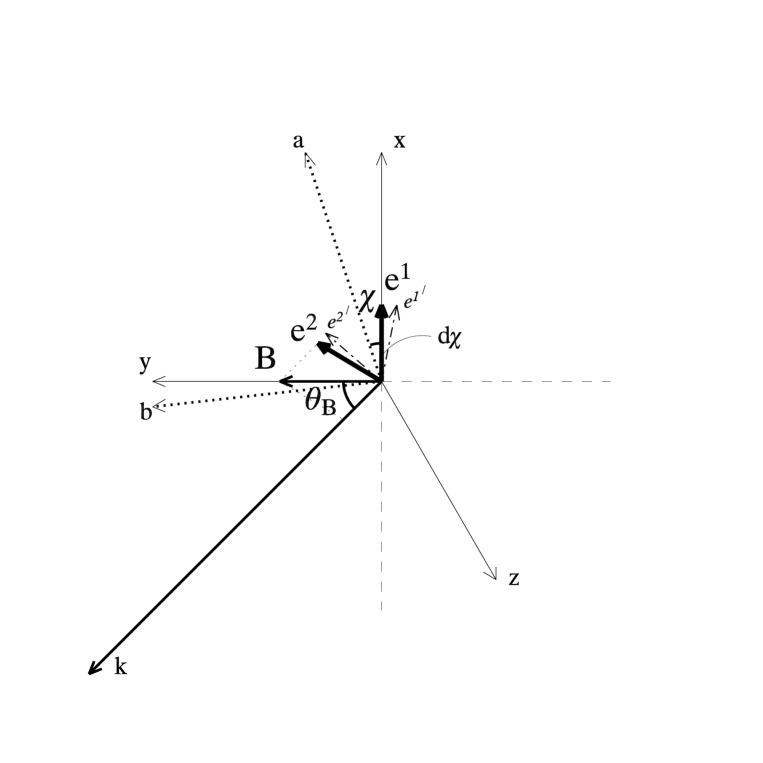
Figure 1: Sketch map of polarization in synchrotron radiation: vectors ${\rm k}$, ${\rm B}$, ${\rm e}^{1}$, and ${\rm e}^{2}$ represent the wave vector, magnetic field, e-mode, and o-mode, respectively. $\chi$ and $d\chi$ respectively represent the EVPA defined in arbitrary coordinate system $(a,b)$ and the change of EVPA due to radiation transfer effect. See text for detail.

The synchrotron radiation from an individual particle is elliptically polarized. The major axis of the polarization ellipse e¹ is perpendicular to the plane spanned by the magnetic vector B and the wave vector k, and the minor axis e${}^{2}\propto$ k$\times$e¹ is perpendicular to the major axis and wave vector. The electric field component of the radiation can be projected along the major and minor axes, namely the e- and o-component, respectively. Figure 1 shows the corresponding geometry in the three dimensional (3D) Cartesian coordinates $(x,y,z)$:

$${\rm\bf B}/B = (0,\,1,\,0),\qquad{\rm\bf k}/k\quad=\quad(0,\,\cos\theta_{B},\,\sin\theta_{B}),$$

$${\rm\bf e}^{1} = (1,\,0,\,0),\qquad\quad{\rm\bf e}^{2}\quad=\quad(0,\,\sin\theta_{B},\,-\cos\theta_{B}),$$ (1)

where $\theta_{B}$ is the angle between B and k, and $k$ and $B$ are the wave number and the amplitude of the magnetic field, respectively. For a population of relativistic particles with a smooth pitch angle distribution, the circular polarization (CP) component of synchrotron emission almost cancels out, and the emissivity of the e-component is generally much greater than that of the o-component. Therefore, the synchrotron radiation from a population of relativistic particles is often treated as partially linearly polarized along e¹. The e-component base ${\rm\bf e}^{1}$ then indicates the electric vector of the linearly polarized (LP) radiation. Since the CP component does not cancel out exactly, sometimes it is more convenient to use the right-handed and left-handed CP bases

$$\mathrm{\bf e}^{R} = \frac{1}{\sqrt{2}}(\mathrm{\bf e}^{1}+i\mathrm{\bf e}^{2}),\qquad\mathrm{\bf e}^{L}\quad=\quad\frac{1}{\sqrt{2}}(\mathrm{\bf e}^{1}-i\mathrm{\bf e}^{2}).$$ (2)

According to the intensity matrix $\mathcal{I}^{ij}$ defined by Melrose (1971) with an arbitrary orthogonal bases, the total intensity is given by

$$I = \mathrm{trace}(\mathcal{I}^{ij})\quad=\quad\mathcal{I}^{11}+\mathcal{I}^{22}\quad=\quad\mathcal{I}^{RR}+\mathcal{I}^{LL}.$$ (3)

Then one has the formal polarization vector $\vec{p}=(p_{Q},p_{U},p_{V})$ introduced by Landi Degl’Innocenti & Landolfi (2004)

$$p_{Q} = \frac{\mathcal{I}^{11}-\mathcal{I}^{22}}{\mathcal{I}^{11}+\mathcal{I}^{22}},$$

$$p_{U} = \frac{\mathcal{I}^{12}+\mathcal{I}^{21}}{\mathcal{I}^{11}+\mathcal{I}^{22}},$$

$$p_{V} = \frac{i(\mathcal{I}^{12}-\mathcal{I}^{21})}{\mathcal{I}^{11}+\mathcal{I}^{22}}\quad=\quad\frac{\mathcal{I}^{RR}-\mathcal{I}^{LL}}{\mathcal{I}^{RR}+\mathcal{I}^{LL}},$$ (4)

The total polarization fraction $\Pi$, CP fraction $\Pi_{C}$, LP fraction $\Pi_{L}$, and the electric vector position angle (EVPA) $\chi_{0}$ are then given by

$$\Pi = \left[1-\frac{4\mathrm{det}(\mathcal{I}^{ij})}{\mathrm{trace}(\mathcal{I}^{ij})^{2}}\right]^{1/2},$$

$$\Pi_{C} = p_{V},$$

$$\Pi_{L} = (\Pi^{2}-\Pi_{C}^{2})^{1/2}\quad=\quad(p_{Q}^{2}+p_{U}^{2})^{1/2},$$

$$\tan 2\chi_{0} = \frac{p_{U}}{p_{Q}}\,.$$ (5)

The normalized polarization vector can be rewritten in the form of the 4D Stokes vector as $\vec{S}=(I,Q,U,V)^{T}=I(1,p_{Q},p_{U},p_{V})^{T}$. The Stokes vector, the intensity matrix, and ($I$, $\Pi_{C}$, $\Pi_{L}$, $\chi_{0}$) all give a complete description of the properties of partially polarized emission.

In order to describe the polarized radiative transfer in highly-magnetized plasma, Landi Degl’Innocenti & Landolfi (2004) introduce another three 3D formal vector $\vec{\epsilon},\vec{\eta},\vec{\rho}$, where $\vec{\epsilon}$ is the normalized emission vector, which is related to the 4D emission coefficient $\vec{\varepsilon}=(\varepsilon_{I},\varepsilon_{Q},\varepsilon_{U},\varepsilon_{V})^{T}$: $\vec{\epsilon}\equiv(\epsilon_{Q},\epsilon_{U},\epsilon_{V})=(\varepsilon_{Q},\varepsilon_{U},\varepsilon_{V})/I$, $\vec{\eta}\equiv(\eta_{Q},\eta_{U},\eta_{V})$ is the absorption vector, and $\vec{\rho}$ is the Faraday rotation vector. The total emission and average absorption coefficients are represented by $\varepsilon_{I}=\epsilon_{I}I$ and $\eta_{I}$, respectively. Then the transfer of polarized emission is described with

$${{\rm d}I\over{\rm d}\rm s} = -(\eta_{I}+\vec{\eta}\cdot\vec{p}-\epsilon_{I})I,$$

$${{\rm d}\vec{p}\over{\rm d}\rm s} = -\vec{\eta}+(\vec{\eta}\cdot{}\vec{p})\vec{p}+\vec{\rho}\times\vec{p}+\vec{\epsilon}-\epsilon_{I}\vec{p}\,,$$ (6)

which govern the evolution of the polarization properties of radiation through a magnetized plasma. These equations can be rewritten in the form of Stokes vector as

$$\frac{\rm d}{\rm d\rm s}\vec{S} = \vec{\varepsilon}\quad-\quad\mathbf{K}\vec{S},$$ (7)

or explicitly

$$\frac{\rm d}{\rm d\rm s}\left(\begin{array}[]{cccc}I\\ Q\\ U\\ V\end{array}\right) = \left(\begin{array}[]{cccc}\varepsilon_{I}\\ \varepsilon_{Q}\\ \varepsilon_{U}\\ \varepsilon_{V}\end{array}\right)\quad-\quad\left(\begin{array}[]{cccc}\eta_{I}&\eta_{Q}&\eta_{U}&\eta_{V}\\ \eta_{Q}&\eta_{I}&\rho_{V}&-\rho_{U}\\ \eta_{U}&-\rho_{V}&\eta_{I}&\rho_{Q}\\ \eta_{V}&\rho_{U}&-\rho_{Q}&\eta_{I}\end{array}\right)\left(\begin{array}[]{cccc}I\\ Q\\ U\\ V\end{array}\right).$$ (24)

One can use the rotation matrix

$$\mathrm{R}(\chi) = \left(\begin{array}[]{cccc}1&0&0&0\\ 0&\cos 2\chi&\sin 2\chi&0\\ 0&-\sin 2\chi&\cos 2\chi&0\\ 0&0&0&1\end{array}\right),$$ (29)

to transform the Stokes vector from the coordinates $({\rm\bf e}^{1},{\rm\bf e}^{2})$ to the reference coordinates $({\bf a},{\bf b})$, where a corresponds to the North at the observer and b corresponds to the East (see Figure 1). Then we have

$$\frac{\rm d}{\rm d\rm s}\vec{S}^{\prime} = \vec{\varepsilon}^{\prime}\quad-\quad\mathbf{K}^{\prime}\quad\vec{S}^{\prime}\,,$$ (30)

where $\vec{S}^{\prime}=\mathrm{R}(\chi)\vec{S}$, $\vec{\varepsilon}^{\prime}=\mathrm{R}(\chi)\vec{\varepsilon}$, and $\mathbf{K}^{\prime}=\mathrm{R}(\chi)\mathbf{K}\mathrm{R}(-\chi)$.

2.2 Synchrotron Emission, Absorption, and Faraday Coefficients

For a population of relativistic electrons in the Maxwell distribution, i.e., relativistic thermal distribution, with the number density $N_{0}$ and temperature $T_{e}\gg m_{e}c^{2}/k$, the distribution function with respect to the electron energy $E$ is

$$N(E) = N_{0}\frac{E^{2}}{2(kT_{e})^{3}}\mathrm{exp}(-E/kT_{e})\,,$$ (31)

where $m_{e}$, $c$, and $k$ are the electron mass, speed of light, and Boltzmann constant, respectively. In the coordinates of (e¹, e²), the four synchrotron emission coefficients are (Sazonov, 1969; Pacholczyk, 1970; Melrose, 1971)

$$\varepsilon_{I} = \frac{e^{2}m_{e}^{2}c^{3}}{\sqrt{3}}\frac{N_{0}}{2(kT_{e})^{2}}\nu I_{I}(x_{M}),$$

$$\varepsilon_{Q} = \frac{e^{2}m_{e}^{2}c^{3}}{\sqrt{3}}\frac{N_{0}}{2(kT_{e})^{2}}\nu I_{Q}(x_{M}),$$

$$\varepsilon_{U} = 0,$$

$$\varepsilon_{V} = \frac{4e^{2}m_{e}^{3}c^{5}\mathrm{cot}\theta_{B}}{3\sqrt{3}}\frac{N_{0}}{2(kT_{e})^{3}}\nu I_{V}(x_{M})\,,$$ (32)

where $e$ is the elementary charge units and $x_{M}$ is the ratio of the emission frequency $\nu$ to the characteristic frequency $\nu_{c}={3eB\mathrm{sin}\theta_{B}(kT_{e})^{2}}/{4\pi m_{e}^{3}c^{5}}$, and the integrations $I_{I},I_{Q}$ and $I_{V}$ can be calculated with the aid of the modified Bessel functions $K_{\alpha}(z)$:

$$F(x) = x\int_{x}^{\infty}K_{5/3}(z)dz\,,$$

$$G(x) = xK_{2/3}(x)\,,$$

$$H(x) = xK_{1/3}(x)+\int_{x}^{\infty}K_{1/3}(z)dz,\quad$$

$$I_{I}(x_{M}) = \frac{1}{x_{M}}\int_{0}^{\infty}z^{2}\mathrm{exp}(-z)F\left(\frac{x_{M}}{z^{2}}\right)dz\,,$$

$$I_{Q}(x_{M}) = \frac{1}{x_{M}}\int_{0}^{\infty}z^{2}\mathrm{exp}(-z)G\left(\frac{x_{M}}{z^{2}}\right)dz\,,$$

$$I_{V}(x_{M}) = \frac{1}{x_{M}}\int_{0}^{\infty}z^{\quad}\mathrm{exp}(-z)H\left(\frac{x_{M}}{z^{2}}\right)dz\,.$$ (33)

The emission coefficients along the two axes ${\rm\bf e}^{1}$ and ${\rm\bf e}^{2}$ are given, respectively, by

$$\varepsilon_{1} = \frac{\varepsilon_{I}+\varepsilon_{Q}}{2},$$

$$\varepsilon_{2} = \frac{\varepsilon_{I}-\varepsilon_{Q}}{2}.$$ (34)

The absorption coefficient can be calculated with the Kirchhoff’s law

$$\frac{S}{2} = \frac{\varepsilon_{1}}{\eta_{1}}=\frac{\varepsilon_{2}}{\eta_{2}}\,,$$

$$\eta_{I} = \frac{\eta_{1}+\eta_{2}}{2}\,,$$

$$\vec{\eta} = \frac{(\varepsilon_{Q},\,\varepsilon_{U},\,\varepsilon_{V})}{S}=\frac{\vec{\epsilon}I}{S}\,,$$ (35)

where $S=\varepsilon_{I}/\eta_{I}$ is the source function, $S=B_{\nu}=2h\nu^{3}/c^{2}[\exp{(h\nu/kT_{e})}-1]$ for a thermal distribution, and $h$ is the Planck constant.

According to Melrose (1997), the high-frequency waves may be treated as two transverse nature wave modes with dispersion relations

$$k_{\pm}^{2}c^{2}-\omega^{2}=\frac{1}{2}\{\alpha^{11}+\alpha^{22}\pm[(\alpha^{11}-\alpha^{22})^{2}+4\alpha^{12}\alpha^{21}]^{1/2}\},$$

where $\omega=2\pi\nu$, $k$ is the wave number, and the response tensor $\alpha^{ij}$ satisfies $\alpha^{12}=-\alpha^{21}$. The polarization vectors of the two natural modes are then given by

$${\rm\bf e}^{\pm}=\frac{T_{\pm}{\rm\bf e}^{1}+i{\rm\bf e}^{2}}{\sqrt{1+T_{\pm}^{2}}}, T_{\pm}=\frac{\alpha^{11}-\alpha^{22}\mp[(\alpha^{11}-\alpha^{22})^{2}+4\alpha^{12}\alpha^{21}]^{1/2}}{2i\alpha^{12}},$$ (36)

which are two orthogonal elliptically polarized modes with axial ratios $T_{\pm}$. Note that $T_{+}T_{-}=-1$ implying that the two natural modes have identical ellipticity and opposite handedness. The electric vector ${\rm\bf E}$ of any wave can be decomposed on the bases of the two natural modes as $E_{+}{\rm\bf e}^{+}+E_{-}{\rm\bf e}^{-}$ or on the bases of the two LP modes as $E_{1}{\rm\bf e}^{1}+E_{2}{\rm\bf e}^{2}$. Then

$$E_{1}=E_{+}\frac{T_{+}}{\sqrt{1+T_{+}^{2}}}+E_{-}\frac{T_{-}}{\sqrt{1+T_{-}^{2}}}$$

and

$$E_{2}=E_{+}\frac{1}{\sqrt{1+T_{+}^{2}}}+E_{-}\frac{1}{\sqrt{1+T_{-}^{2}}}.$$

Using the definitions in equation (2), a third decomposition can be made on two CP modes as $E_{R}{\rm e}^{R}+E_{L}{\rm e}^{L}$, with

$$E_{R}=E_{+}\frac{T_{+}+1}{\sqrt{2(1+T_{+}^{2})}}+E_{-}\frac{T_{-}+1}{\sqrt{2(1+T_{-}^{2})}}$$

and

$$E_{L}=E_{+}\frac{T_{+}-1}{\sqrt{2(1+T_{+}^{2})}}+E_{-}\frac{T_{-}-1}{\sqrt{2(1+T_{-}^{2})}}.$$

The total emission coefficient $\varepsilon_{I}$ is proportional to $E^{2}$, i.e.,

$$\varepsilon_{I} = \Bigg{\{}\begin{array}[]{ccc}\varepsilon_{+}+\varepsilon_{-}\quad\propto\quad E_{+}^{2}+E_{-}^{2}\\ \varepsilon_{1}+\varepsilon_{2}\quad\propto\quad E_{1}^{2}+E_{2}^{2}\\ \varepsilon_{R}+\varepsilon_{L}\quad\propto\quad E_{R}^{2}+E_{L}^{2}\end{array}.$$ (40)

Then the LP and CP emission coefficients ($\varepsilon_{Q}$ and $\varepsilon_{V}$) are given by

$$\varepsilon_{Q} = \varepsilon_{1}-\varepsilon_{2}=\varepsilon_{Q+}+\varepsilon_{Q-}=\frac{T_{+}^{2}-1}{1+T_{+}^{2}}\varepsilon_{+}+\frac{T_{-}^{2}-1}{1+T_{-}^{2}}\varepsilon_{-}=\frac{T_{+}+T_{-}}{T_{+}-T_{-}}(\varepsilon_{+}-\varepsilon_{-})$$

$$\varepsilon_{V} = \varepsilon_{R}-\varepsilon_{L}=\varepsilon_{V+}+\varepsilon_{V-}=\frac{2T_{+}}{1+T_{+}^{2}}\varepsilon_{+}+\frac{2T_{-}}{1+T_{-}^{2}}\varepsilon_{-}=\frac{2}{T_{+}-T_{-}}(\varepsilon_{+}-\varepsilon_{-}),$$ (41)

which implies that

$$\frac{\varepsilon_{V}}{\varepsilon_{Q}} = \frac{2}{T_{+}+T_{-}}=\frac{2i\alpha^{12}}{\alpha^{11}-\alpha^{22}}=\frac{\rho_{\rm RM}}{\rho_{\rm RRM}},$$ (42)

where $\rho_{\rm RM}=i\alpha^{12}/2\omega c$ is called the rotation measure, or the Faraday rotation coefficient, and $\rho_{\rm RRM}=(\alpha^{11}-\alpha^{22})/4\omega c$ is called the relativistic rotation measure, or the Faraday conversion coefficient. Note that $\varepsilon_{\pm}^{2}=\varepsilon_{Q\pm}^{2}+\varepsilon_{V\pm}^{2}$, $\varepsilon_{\pm}/\eta_{\pm}=S/2$, $\eta_{Q}=\varepsilon_{Q}/S=(\eta_{Q+}+\eta_{Q-})/2$, $\eta_{V}=\varepsilon_{V}/S=(\eta_{V+}+\eta_{V-})/2$.

In a uniform plasma, $\vec{\rho}=(2\rho_{\rm RRM},0,2\rho_{\rm RM})$ and the three formal vector $\vec{\epsilon}$, $\vec{\eta}$, and $\vec{\rho}$ are parallel to each other. If there is no external radiation, the term $(\vec{\rho}\times\vec{p})$ in equations (2.1) vanishes (Landi Degl’Innocenti & Landolfi, 2004; Bekefi, 1966; Kennett & Melrose, 1998) and one has the solution with $\vec{p}$ also parallel to these vectors. Then equations (2.1) become

$${{\rm d}I\over{\rm d}\rm s} = -[(1+\Pi\Pi_{0})\eta_{I}-\epsilon_{I}]I=-\left[(1+\Pi\Pi_{0})\frac{I}{S}-1\right]\varepsilon_{I}\,,$$

$${{\rm d}\Pi\over{\rm d}\rm s} = \eta_{I}\Pi_{0}(\Pi^{2}-1)+\epsilon_{I}(\Pi_{0}-\Pi)=\left[\frac{\Pi_{0}(\Pi^{2}-1)}{S}+\frac{\Pi_{0}-\Pi}{I}\right]\varepsilon_{I}\,,$$ (43)

where $\Pi_{0}=(\varepsilon_{Q}^{2}+\varepsilon_{U}^{2}+\varepsilon_{V}^{2})^{1/2}/\varepsilon_{I}$ is the polarization fraction of an optically thin source. Note that in this case, if we denote the unit vector along $\vec{\epsilon}$ as $\vec{u}$, then $\vec{p}=\Pi\vec{u}$, $\vec{\epsilon}=\Pi_{0}\epsilon_{I}\vec{u}$, $\vec{\eta}=\vec{\epsilon}I/S=\Pi_{0}\eta_{I}\vec{u}$. With the increase of the optical depth, we see that $\Pi$ decreases, and the existence of $\Pi$ enhances the self-absorption by a factor of $1+\Pi\Pi_{0}$.

Therefore, in a uniform plasma, besides the source function that is determined by the particle distribution, there are four independent coefficients. From the three emission coefficients given by equations (2.2) and the Faraday rotation coefficient $\rho_{V}=2\rho_{\rm RM}$, one can derive the absorption and Faraday conversion coefficients with equations (2.2) and (42), respectively. Melrose (1997) derived the three emission coefficients and two Faraday coefficients separately. It appears that his results are not exactly in agreement with equation (42). Neither is the $\rho_{\rm RM}$ and $\rho_{\rm RRM}$ obtained by Shcherbakov (2008). All these calculations invoke some approximations to simplify the Trubnikov’s linear response tensor. While equation (42) is derived from very general theoretical considerations without any approximations. We therefore stand by our approach of deriving $\rho_{\rm RRM}$ from $\rho_{\rm RM}$ and the emission coefficients in a previous paper (Huang et al., 2008).

Melrose (1997) gives $\rho_{\rm RM}$ for thermal plasmas in the cold ($\gamma_{C}=kT_{e}/m_{e}c^{2}+1\approx 1$) and extremely relativistic (ER) ($\gamma_{C}\gg 1$) limits:

$$\rho_{\rm RM}^{{\rm C}} = \frac{e^{3}N_{0}B\cos\theta_{B}}{2\pi\gamma_{c}m_{e}^{2}c^{2}\nu^{2}},$$

$$\rho_{\rm RM}^{{\rm ER}} = \frac{\ln\gamma_{c}}{2\gamma_{c}}\frac{e^{3}N_{0}B\cos\theta_{B}}{2\pi\gamma_{c}m_{e}^{2}c^{2}\nu^{2}}.$$ (44)

We use the following extrapolation to obtain $\rho_{\rm RM}$ for arbitrary electron temperatures

$$\rho_{\rm RM} = \gamma_{c}^{-1}(\rho_{\rm RM}^{{\rm C}}-\rho_{\rm RM}^{{\rm ER}})+\rho_{\rm RM}^{{\rm ER}}\,,$$ (45)

which is simple and accurate enough according to Shcherbakov (2008). For cold plasmas, cyclotron emission dominates, $\varepsilon_{I}>\varepsilon_{V}\gg\varepsilon_{Q}$, and $\rho_{V}\gg\rho_{Q}$. For hot plasmas, synchrotron emission dominates, $\epsilon_{I}>\epsilon_{Q}\gg\epsilon_{V}$, and $\rho_{Q}\gg\rho_{V}$.

For a given ray, the magnetic field structure of the accretion flow determines the coordinates (e¹, e²). For given reference directions of the North and East, we also obtain the coordinates (a, b). One therefore can use the coefficients obtained above in the coordinates of (e¹, e²) to obtain the contributions of this ray to the Stokes parameters in the coordinates of (a, b).

2.3 General Relativistic Radiative Transfer

In magnetized plasmas around black holes, photons experience both the general relativistic light bending and plasma birefringence effects and change their propagation directions. Fanton et al. (1997) showed how photons propagate along the null geodesics near black holes. Broderick & Blandford (2003) discussed how the plasma effect causes refraction, which makes the photon propagation path deviate from the null geodesics. However, such refraction is significant only if either the electron cyclotron frequency $\nu_{B}$ or the electron plasma frequency $\nu_{P}$ is comparable to the observation frequency $\nu_{\mathrm{obs}}$. In the observational band (from millimeter to near-infrared band) we are interested in, we always have $\nu_{B}/\nu_{\mathrm{obs}}<10^{-3}$, and $\nu_{P}/\nu_{\mathrm{obs}}<10^{-4}$. Therefore, although we consider the Faraday conversion and rotation effects of magnetized plasmas, we still assume photons of both natural modes propagating along the null geodesics.

We use the ray-tracing code discussed in Huang et al. (2007) to determine the photon trajectory from a specific direction as observed at infinity. Along the trajectory which crosses the emission region, we record the four-wave-vector $k^{\mu}$, accretion flow velocity $u^{\mu}$, electron temperature $T_{e}=\gamma_{c}m_{e}c^{2}/k$, number density $n$, and three magnetic vector $\mathrm{B}^{i}$ at each line element. We convert the three magnetic vector $\mathrm{B}^{i}$ into four-vector $b^{\mu}$ following e.g., Gammie et al. (2003). The four-vectors of the elliptical axes of synchrotron emission $(e^{1\mu},e^{2\mu})$ are calculated the same way as that discussed by Broderick & Blandford (2004). The four-vectors of the reference coordinates $(a^{\mu},b^{\mu})$ are calculated according to the parallel transport in the general relativistic theory with $(a^{t},b^{t})$ arbitrarily set as $(0,0)$ (Chandrasekhar, 1983). The Stokes parameters are not conserved along the photon trajectories due to gravitational effect. However, the photon occupation numbers $\mathcal{N}_{S}=(\mathcal{N}_{I},\mathcal{N}_{Q},\mathcal{N}_{U},\mathcal{N}_{V})$, defined as $\mathcal{N}_{S}=\vec{S}/\nu^{3}$, are Lorentz invariants. Therefore, the radiative transfer equation (7) can be rewritten as

$$\frac{\rm d^{\quad}}{\rm d\ell^{\quad}}\mathcal{N}_{S} = \mathcal{E}\quad-\quad\bf{\mathcal{K}}\mathcal{N}_{S},\qquad(\mathcal{E}=\frac{\vec{\varepsilon}}{\nu^{2}},\qquad\mathcal{K}=\nu\mathbf{K}),$$ (46)

with the differential affine parameter $\rm d\ell=\rm ds/\nu_{\mathrm{obs}}$ and the emission frequency $\nu=-u^{\mu}k_{\mu}$.

3 SIMULATION RESULTS OF POLARIZATIONS

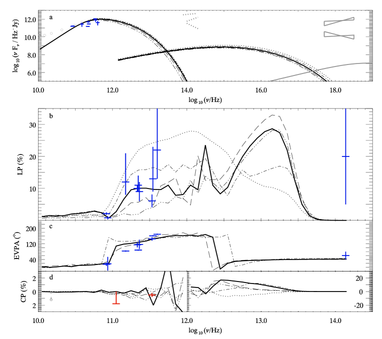
Figure 2: Simulated results from the fiducial model with $\beta_{\nu}=0.7,\beta_{p}=0.4,C_{1}=0.47,\dot{M}=6\times 10^{17}{\rm g\cdot s^{-1}},i=40^{\circ}$, and $\Theta=115^{\circ}$ (solid lines). Models with the same parameters except $i=20^{\circ}$ (3-dots-dashed lines), $30^{\circ}$ (long dashed lines), $i=50^{\circ}$ (dash-dotted lines), and $i=60^{\circ}$ (dotted lines) are shown for comparison. Data are from Aitken et al. (2000); Bower et al. (2005); Macquart et al. (2006); Marrone et al. (2006); Eckart et al. (2006), Bower et al. (2001); Marrone et al. (2006), Baganoff et al. (2001),etc.. (a) spectrum of synchrotron, SSC radiation (thick) and bremsstrahlung radiation (thin); (b) linear polarization degrees; (c) EVPA; (d) circular polarization degrees.

In this section, we present our simulation results in detail. The data we adopt are mainly from (multi-epoch) linear polarization observations reported by Aitken et al. (2000); Bower et al. (2005); Macquart et al. (2006); Marrone et al. (2006), and Eckart et al. (2006), marked with crosses in Panels (a), (b), and (c) of Figure 2. Two circular polarization data in Panel (d) are from Bower et al. (2001) and Marrone et al. (2006). The ties in X-ray band are from Baganoff et al. (2001). Other data of luminosity shown in Panel (a) are the same adopted in Huang et al. (2008).

3.1 Configuration of the Magnetic Field

We adopt the two-temperature magneto-rotational instability (MRI) driven Keplerian accretion flow model of magnetized plasmas around the central black hole in Sgr A* [see in Liu et al. (2007a, b) for details]. A black hole mass of $M_{\mathrm{BH}}=4.1\times 10^{6}M_{\odot}$, where $M_{\odot}$ is the solar mass, is recently derived from observations of the orbital motion of the short-period star S0-2 (Ghez et al., 2008). The corresponding model parameters include the ratio of the viscous stress to the magnetic field energy density $\beta_{\nu}$ [fixed at $0.7$, see Pessah et al. (2006)], the ratio of the magnetic field energy density to the gas pressure $\beta_{p}$, the electron heating rate indicated by a dimensionless parameter $C_{1}$, the mass accretion rate $\dot{M}$, the inclination angle $i$ and the position angle $\Theta$ of the axis perpendicular to the equatorial plane of the accretion flow. In this model, thermal electrons are energised by sound waves with the heating rate given by $\tau_{\rm ac}^{-1}=c_{S}^{2}/3C_{1}H\langle v_{e}\rangle$, where $c_{S}$, $H$, and $\langle v_{e}\rangle$ are the sound speed, the scale height of the accretion flow, and the mean speed of the electrons, respectively, and we have assumed that the scattering mean free path of the electrons by the sound waves is scaled with $H$. A comparison of this heating model with other two-temperature models (Yuan et al., 2003) can be found in Liu et al. (2007b).

MHD simulations of the MRI show that the magnetic field is dominated by its azimuthal component due to the shearing motion of the Keplerian accretion flow. Previous pseudo-Newtonian modelling of the sub-millimeter to NIR polarization of Sgr A* has assumed that the magnetic field does not have vertical and radial components (Melia et al., 2001; Bromley et al., 2001; Liu et al., 2007a). Here we consider more realistic configurations. Most MRI simulations adopt poloidal or toroidal magnetic field loops confined to an initial torus of matter (Hawley & Balbus, 2002; Gammie et al., 2003). Simulations with initial magnetic field lines perpendicular to the disk plane tend to produce stronger magnetic fields in the final quasi-steady state (Pessah et al., 2006). The field lines are dragged and twisted due to the Keplerian motion of the accretion flow. If there is a large scale poloidal magnetic field, the field lines will be nearly parallel (anti-parallel) to the velocity field in the upper half to the equatorial plane and anti-parallel (parallel) in the lower half. We will adopt such a mean magnetic field configuration in the following.

3.2 The Fiducial Model

We first obtain a fiducial model to the spectrum, linear polarization (LP) fraction, electric vector position angle (EVPA), and circular polarization (CP) fraction with $\beta_{p}=0.4$, $C_{1}=0.47$, $\dot{M}=6\times 10^{17}\mathrm{g}\cdot\mathrm{s}^{-1}$, $i=40^{\circ}$, and $\Theta=115^{\circ}$. No external Faraday rotation measure is introduced. The corresponding results are shown by the solid lines in Panels (a),(b),(c), and (d) of Figure 2, respectively. It is consistent with the fiducial model in Huang et al. (2008). This Keplerian accretion flow reproduces the emission in the millimeter to sub-millimeter bump of Sgr A*, but underestimates the emission in the NIR and X-ray bands. The thick solid lines in Figure 2 (a) represent the synchrotron (to the left) and synchrotron self-Comptonization (SSC, in the middle) radiation components, and the thin solid line to the right represents the bremsstrahlung radiation. This result is different from that of Liu et al. (2007), where they are able to reproduce the observed NIR flux level. In their model, an un-polarized jet/outflow component were introduced, which effectively suppresses the LP below 100 GHz (Liu et al., 2007a). We don’t have such a component here. The onset frequency of the LP therefore constrains the model parameter space so that the model predicted NIR and X-ray fluxes are more than one order of magnitude lower than the observed values. The quiescent-state X-ray emission is extended and has been attributed to thermal emission from plasmas near the capture radius (Baganoff et al., 2003; Quataert, 2004; Xu et al., 2006). The X-ray emission from our accretion flow at small radii should be lower than the observed value. However, there is evidence for a quiescent-state NIR emission from the direction of Sgr A* (Do et al., 2009). This emission can be caused by smaller flares or a quasi-stationary emission component. If it is indeed powered by the accretion flow at small radii, it must be dominated by emission regions within $6GM_{\rm BH}/c^{2}$, where $G$ is the gravitational constant and $c$ is the speed of light, or associated with outflows, which may also be responsible for the long wavelength radio emissions.

As shown in Figure 2 (b) and (c), the LP fraction is a few percent in the centimeter bands. It can be reduced to the observed level either by depolarization of an external medium or through the dominance of an un-polarized emission component from a jet/outflow component. In this band, only the red-shifted side of the accretion flow is optically thin. Hence, the EVPA is perpendicular to the accretion flow axis projection, since the magnetic field is toroidal and the emission is dominated by the extraordinary mode. When the observational frequency increases to $\sim$100GHz, the LP degree increases because the Faraday rotation and Faraday conversion coefficients decrease with the observation frequency $\nu$ as $\nu^{-2}$ and $\nu^{-3}$, respectively. At the same frequency, the near and far sides of the accretion flow become optically thin and dominate the polarized emission so that EVPA preforms a $\sim 90^{\circ}$ flip to be parallel to the disk axis projection. In the sub-millimeter band, the LP degree increases to $\sim 10\%$, explaining observations well. Furthermore, the EVPA has a small increase of $\sim 20^{\circ}$ in this band. With further increasing of the observational frequency, the blue-shifted side finally become optically thin at $\sim 2-3$ THz, making the whole disk optically thin with its blue-shifted side being the dominant emission region. Thus, the EVPA flips back to be perpendicular to the axis projection again. In the quiescent state discussed in this paper, there is almost zero polarization in the NIR band because the non-polarized SSC emission component dominates. However, the EVPA is still meaningful for flaring activities dominated by the synchrotron emission.

The predicted CP fraction is shown in Figure 2 (d). The CP degree is nearly zero in the centimeter bands, so that the observed CP fraction of several percents (Bower et al. 2002) might be attributed to a jet/outflow component (Beckert & Falcke 2002). At sub-millimeter and shorter wavelengths, however, the CP amplitude increases gradually, then significantly to greater than $10\%$ at $\sim$1 THz. We show the CP fraction in different scales for clarity of presentation here. Notice that the LP fraction also has some oscillations in the same band. These high LP and CP may be due to the combination of the general relativity and birefringence effects, and can be tested with future THz polarization observations.

Interestingly in the millimeter to sub-millimeter band, the CP degree is mostly negative, i.e., the polarization is left-handed. Here, we adopt two observational data for CPs, a limit of $-1.8\%$ at 112 GHz reported by Bower et al. (2001) and a detection of $\sim-0.5\%\pm 0.3\%$ at 340GHz by Marrone et al. (2006) (both marked with red crosses). Although they mentioned that the detections were quite uncertain due to weather conditions and instrumental effects, the left-handed properties seemed to be real. Our model therefore reproduces the CP observations. However, we notice that the CP degree is very sensitive to the magnetic field structure and model parameters. Thus, our predictions here should be interpreted with precautions.

3.3 The Inclination Angle Dependence

The dependence of these results on the inclination angle $i$ is also shown in Figure 2 with the corresponding models indicated in the legend of Panel (b). The other model parameters have been fixed here. Results for $i=20^{\circ}$, $30^{\circ}$, $50^{\circ}$, and $60^{\circ}$ are shown with the 3-dots-dashed, long dashed, dot-dashed, and dotted lines, respectively. Different from the pseudo-Newtonian cases [see Liu et al. (2007a)], the changes in the inclination angle slightly affect the centimeter polarization and high frequency flux density. This is due to two effects: absorption of emission from the edge of accretion flow and amplification of emission by the GR light bending.

However, the inclination angle affects the LP degree significantly. Generally speaking, the onset frequency of high LP decreases and the LP degree in sub-millimeter band increases with the increase of the inclination angle. This is because the projected magnetic field lines are close to parallel lines in the nearly edge-on case while becoming circular helices in the nearly face-on case. Parallel magnetic field lines result in the highest LP degree (up to $30\%$ in sub-millimeter band), while circular helices result in a zero LP degree due to the rotation symmetry of the flow. The observed LP degrees in the sub-millimeter band remain stable at $\sim 10\%$ since its discovery (Aitken et al., 2000), which provides a constraint of $\sim 40^{\circ}\pm 10^{\circ}$ on the inclination angle of the Keplerian accretion flow.

For the EVPA, it flips at a lower frequency for the first time and a higher frequency again. This is because the near side of the inclined disk dominates the emission in a wider band. For the $i=60^{\circ}$ case, the near side dominates after the first flip, and the second flip doesn’t appear until the frequency increases to the NIR band. The second flip may disappear in the band we are interested in for higher values of the inclination angle. The second flip between sub-millimeter band to NIR band is quite important. A stable difference of $\sim 80^{\circ}$ in the EVPAs between 230GHz and $\lambda$ 2.2$\mu$m has been observed, which suggests a stable geometry for the accretion plasma around Sgr A* if the NIR emission also originates from the disk. Comparing the fiducial model and the other four cases shown in Fig.2, a mildly-inclined $i\sim 40^{\circ}$ accretion flow appears to better reproduce such a difference in the EVPA caused by changes in optical depth across the emission structure. However, Meyer et al. (2007) derived a highly-inclined $i\gtrsim 70^{\circ}$ disk to obtain significantly variable light-curves in the NIR band. The NIR flare emission was associated with a bright spot orbiting the black hole at the last stable orbit of a disk with a toroidal magnetic field similar to our magnetic field configuration. They also assumed that the sub-millimeter emission comes from a jet to explain the EVPA difference, while the jet/outflow component in our model only dominates the emission in millimeter and longer wavelengths. Therefore, the difference of inclination angle predictions is caused by different assumptions of the geometry for the emitting region, which can be checked by future VLBI observations in the sub-millimeter band.

3.4 The Position Angle Dependence

The observed EVPA is related to the position angle ($\Theta$) of the accretion flow axis. Observationally, the EVPAs in the sub-millimeter band show frequent variability, presumably associated with flares. At 230 GHz, however, it was detected as $\sim 117^{\circ}\pm 24^{\circ}$, showing relatively stable values, during several epochs within more than one year (Bower et al., 2005). Marrone et al. (2007) also reported comparable values of the EVPA at 230GHz. At $\lambda$ 2.2$\mu$m, on the other hand, the EVPA is reported to be stable with a value of $60^{\circ}\pm 20^{\circ}$ (Meyer et al., 2007). In the fiducial model, we find $\Theta=114^{\circ}$ so that the predicted EVPA can give a best fit to both measurements at 230GHz and $\lambda$ 2.2 $\mu$m. In practice, values in the range of $\sim 115^{\circ}\pm 20^{\circ}$ are all acceptable. Interestingly, we find that the predicted first flip in the EVPA also fits the multi-epoch detections at 86 GHz well (Macquart et al., 2006). Moreover, Marrone et al. (2007) observed the EVPA at 340GHz simultaneously with that at 230GHz and reported an averaged $\sim 30^{\circ}$ increase from 230 GHz to 340 GHz. Our model also reproduces this increase in the sub-millimeter band. Meyer et al. (2007) derived a $\Theta$ of $\sim 110^{\circ}$, which is consistent with ours, although their emission model is quite different.

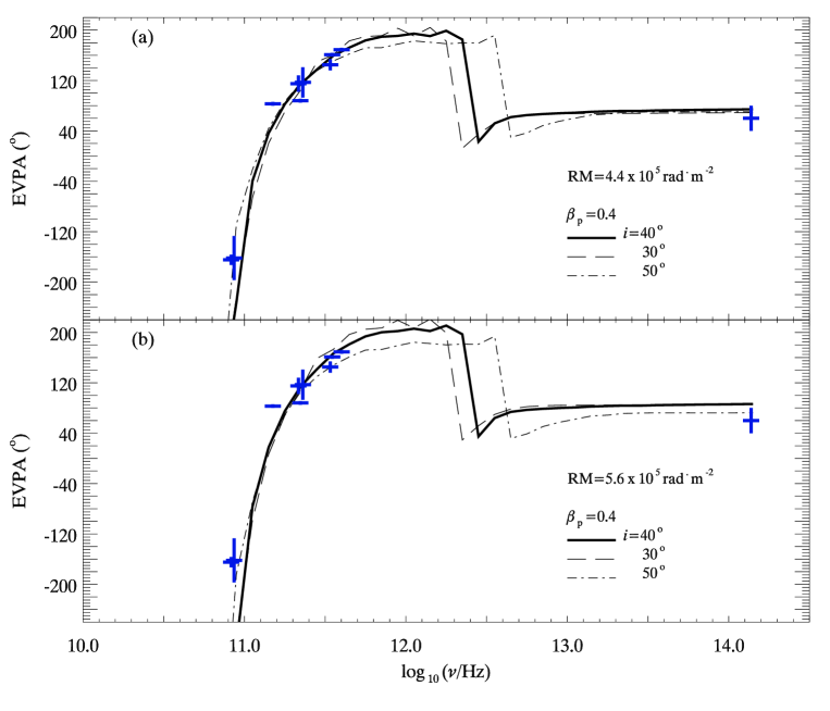
Figure 3: Results of EVPA three models in Fig.2 with external rotation measure of (a) $4.4\times 10^{5}{\rm rad}\cdot{\rm m}^{-2}$ (Macquart et al., 2006) and (b) $5.6\times 10^{5}{\rm rad}\cdot{\rm m}^{-2}$ (Marrone et al., 2007) considered.

Notice that we have assumed that all the observed EVPAs are intrinsic to the accretion flow, i.e., the depolarization and Faraday rotation only occur in the accretion region of Sgr A*. It is likely that the emission from the accretion flow may experience depolarization and Faraday rotation by an external medium described with a rotation measure (RM) $=4.4\times 10^{5}\mathrm{rad}\cdot\mathrm{m}^{2}$ derived from millimeter to sub-millimeter observations (Macquart et al., 2006). In Panel (a) of Figure 3, we plot the corresponding EVPAs of three well-fit models in Figure 2, with different position angles. Multi-epoch observations of the EVPA from $\lambda=$ 3 mm to $\lambda=$ 2.2 $\mu$m can be reproduced with $\Theta=147^{\circ}$ for the fiducial model. Fits with another RM of $5.6\times 10^{5}\mathrm{rad}\cdot\mathrm{m}^{2}$ derived by Marrone et al. (2007) from their simultaneous observations at $230$ GHz and $350$ GHz are plotted in Panel (b). $\Theta=159^{\circ}$ for the fiducial model. Obviously, the position angle $\Theta$ depends on the external rotation measure. More observations in the sub-millimeter and NIR bands will show whether an external rotation measure is necessary.

3.5 Dependence on the Mass Accretion Rate

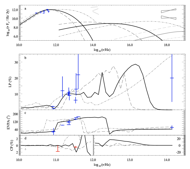
Figure 4: Simulated results for models with $\beta_{p}=0.2$, $\dot{M}=1.5\times 10^{18}$g s^-1 (long-dashed), $\beta_{p}=0.4$ (solid), and $\beta_{p}=0.7$, $\dot{M}=2\times 10^{17}$g s^-1 (dash-dotted), where $\beta_{p}\cdot C_{1}=0.4\cdot 0.47$, and the luminosity in sub-millimeter band does not change significantly.

For these radiatively inefficient accretion flows, the gas pressure is dominated by proton and ions, which have a relatively high temperature Liu et al. (2007). Pessah et al. (2006) showed $\beta_{\nu}\simeq 0.7$. Then both the viscosity (and therefore the mass accretion rate) and the magnetic field energy density are proportional to $\beta_{p}$. The mass accretion rate therefore determines the amplitude of the magnetic field. For a given mass accretion rate, the density is inversely proportional to $\beta_{p}$. Figure 4 shows the dependence of the results on the mass accretion rate, where $\beta_{p}$ and $C_{1}$ are also adjusted to reproduce the millimeter and sub-millimeter spectrum. For $\dot{M}=1.5\times 10^{18}\mathrm{g}\cdot\mathrm{s}^{-1}$, $\beta_{p}=0.2$, $C_{1}=0.94$. The density profile increases by a factor of 5 with respect to the fiducial model. And for a lower accretion rate of $\dot{M}=2\times 10^{17}\mathrm{g}\cdot\mathrm{s}^{-1}$, $\beta_{p}=0.7$, $C_{1}=0.269$. The density profile decreases by a factor of 5.3 with respect to the fiducial model. The inclination angle of the accretion flow is fixed at $40^{\circ}$ and $\Theta$ is obtained by fitting observations at $1.3$ mm and $2.2\mu$ m wavelengths. It can be seen that with the increase of $\dot{M}$ and therefore the magnetic field $B$ and $n$, a lower electron temperature is needed to reproduce the spectrum. This leads to a lower cutoff frequency for both the synchrotron and SSC components. The emission is also strongly self-absorbed so that the onset frequency of strong LP occurs at about 150 GHz. Opposite effects can be seen with the decrease of $\dot{M}$ and there is a higher X-ray emission flux due to the SSC. However, the X-ray flux is still one order of magnitude lower than the observed quiescent-state thermal X-ray emission from a large scale accretion flow (Xu et al. 2005). Even higher NIR and X-ray emission may be produced with further decrease of the mass accretion rate and increase of the electron temperature. However, radio emission will show strong LP. An un-polarized emission component needs to be introduced to suppress the LP to the observed level (Liu et al. 2007).

Moreover, for lower values of $\dot{M}$, the high amplitude of the CP degree starts at lower frequencies, similar to the high LP degrees, e.g., the dash-dotted line shown in Figure 4 (d) with $\beta_{p}=0.7$. Current observations of the LP and CP therefore constrain the $\dot{M}$ to be near $6\times 10^{17}$ g s^-1 with an uncertainty of a factor of $\sim 2$.

3.6 Degeneracy Between the Electron Heating and Magnetic Field

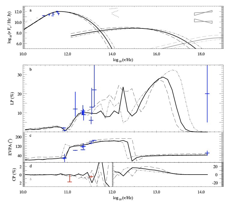
Figure 5: Simulated results from models with $\beta_{p}=0.2$, $C_{1}=0.8$ (dashed) and $\beta_{p}=0.7$ $C_{1}=0.33$ (dot-dashed) with $\dot{M}=6\times 10^{17}{\rm g\cdot s^{-1}}$ and $i=40^{\circ}$ unchanged.

We have shown that the emission spectrum and polarization give good constraints on the orientation of the accretion flow and the mass accretion rate. However, the constraint on the electron heating rate and the magnetic field parameter $\beta_{p}$ is generally poor even with $\beta_{\nu}$ fixed. Figure 5 shows several reproductions to the observed spectrum and polarization with $\dot{M}=6\times 10^{17}$ g s^-1, $\beta_{p}=0.2$; $C_{1}=0.8$ (long-dashed lines), and $\beta_{p}=0.7$; $C_{1}=0.33$ (dashed-dotted lines). The current observations will not be able to distinguish these models. However, there are changes in the SSC and bremsstrahlung components. These can be understood as the following.

For a given $\dot{M}$, the magnetic field is fixed because both of them are proportional to $\beta_{p}N_{0}T_{p}$, where $T_{p}$ is the proton temperature and does not change with $\beta_{p}$. With the increase $\beta_{p}$, we increase the viscosity and therefore the radial velocity. The density will decrease as $N_{0}\propto 1/\beta_{p}$. For a given optically thin synchrotron luminosity required to reproduce the millimeter and sub-millimeter spectral hump, $N_{0}B^{2}T_{e}^{2}$ should not change. Therefore the electron temperature $T_{e}$ should be proportional to $\beta_{p}^{1/2}$. Then with the increase of $\beta_{p}$, the synchrotron spectrum should be slightly harder, i.e., its spectral cutoff $\propto BT_{e}^{2}\propto\beta_{p}$ should shift toward higher frequencies. We therefore expect less low frequency SSC flux density due to the decrease of the electron density. However the SSC component should cut off at a higher frequency, which is proportional to $T_{e}^{2}\propto\beta_{p}$. The SSC luminosity, which is proportional to $N_{0}T_{e}^{2}$, however does not change. To make the SSC cut off in the Chandra X-ray band, we will need to increase $\beta_{p}$ by a factor of $\sim 10$. However, this will reduce the flux density by the same factor. Therefore the SSC component cannot have significant contribution to the observed quiescent state X-ray emission. The bremsstrahlung flux density scales with $N_{0}^{2}/T_{e}^{1/2}\propto\beta_{p}^{-9/4}$. A very low value of $\beta_{p}$ is required for this component to have significant contribution in the X-ray band. There is therefore a degeneracy between the electron heating rate and the magnetic parameter. By introducing a spin parameter to the black hole, the emission volume will be reduced and therefore enhancing the SSC X-ray flux. One may be able to break this degeneracy with the quiescent state NIR and X-ray flux densities.

3.7 Polarized Images in the Millimeter and Sub-Millimeter Bands

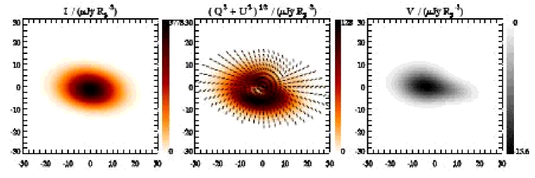
$\lambda=1.3$mm

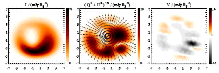
$\lambda=0.86$mm

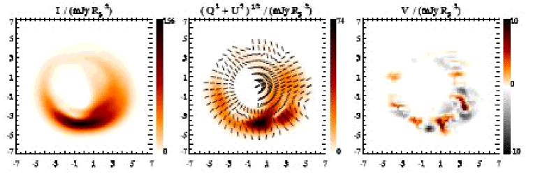
$\lambda=0.6$mm

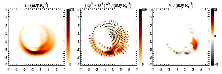
Figure 6: Images of total intensity ($I$), LP emission ($\sqrt{Q^{2}+U^{2}}$), and CP emission ($V$) predicted for Sgr A* at observational wavelengths of 3.5 mm, 1.3 mm, 0.86 mm, and 0.6 mm, from top to bottom, respectively. In images of LP emission, black spurs represent the averaged EVPAs in the nearby regions. In images of CP emission, the left-handed and right-handed regions are respectively presented in grey and red.

Sgr A* is embedded in the inter-stellar medium (ISM) on the Galactic plane. Emission from the accretion flow will experience significant scattering, which smoothes the image without changing its total flux density and polarization properties. We adopt an elliptical Gaussian structure for the scattering screen with a full width of half maximum (FWHM) along its major and minor axis being $\vartheta_{\mathrm{maj}}=(1.39\pm 0.02)(\lambda/1{\rm\ cm})^{2}$ mas and $\vartheta_{\mathrm{min}}=(0.69\pm 0.06)(\lambda/1{\rm\ cm})^{2}$ mas, respectively, and a position angle $\sim 80^{\circ}$ (Shen et al., 2005). The size of the scattering screen becomes smaller with the decrease of the observation wavelength. In practice, the black hole shadow structure is significantly washed out in the millimeter and longer wavelength band by this scattering. However, the scattering becomes less important in sub-millimeter band. We plot images of the total emission $I$, LP :$\sqrt{Q^{2}+U^{2}}$, and CP: $V$ of the fiducial model at several wavelengths $\lambda=$ 3.5mm, 1.3mm, 0.86mm, and 0.6mm in Figure 6. The black dashes in the LP emission represent the EVPAs $\bar{\chi}$. The left-handed and right-handed regions in the CP emission are respectively represented with grey and red color.

The image of the total emission at $\lambda=$ 3.5 mm is smeared by the screening and has an $\sim 80^{\circ}$-oriented elliptical Gaussian structure with the major FWHM of $\sim(0.189\pm 0.003)$mas. This size is consistent with but somewhat smaller than the observation of $\sim 0.21$ mas reported in Shen et al. (2005). The LP and CP emission at $\lambda$ 3.5 mm are also smoothed significantly. The spurs mark the EVPAs, mostly in the radial direction as a result of the toroidal magnetic field configuration. The CP emission is dominated by a grey region representing a left-handed polarization.

Clear black hole shadow structures can be found in images of the total emission at 1.3 mm or shorter wavelengths. Interestingly, clumpy patterns are seen in the sub-millimeter LP with bright and faint regions, and in the CP emission with their left-handed and right-handed regions. Such complex patterns are results of the gravitational light bending and the birefringence effects posing new challenges for future polarization-sensitive VLBI observations.

4 SUMMARY AND DISCUSSION

In this paper we explore the parameter space of the two-temperature MRI driven Keplerian accretion flow model in a non-spin pseudo-Newtonian potential for the time averaged millimeter and shorter wavelength emission from Sgr A* (Liu et al. 2007). The model reproduces the observed emission spectrum and polarization with an inclination angle of $40\pm 10^{\circ}$ and a mass accretion rate of $\sim 6\times 10^{17}$ g s^-1. The former is mostly determined by the amplitude of the LP fraction and the latter is well-constrained by the onset frequency of prominent LP. The LP is low in the centimeter wavelength due to strong self-absorption in the emission region. The orientation of the accretion flow projected on the sky depends on the amplitude of an external Faraday rotation measure. And the model predicted NIR and X-ray fluxes are more than one order of magnitude lower than the observed low flux levels. Although nearly identical millimeter and sub-millimeter spectrum and polarization can be obtained by adjusting the electron heating rate and the magnetic parameter, none of these models can produce NIR and X-ray fluxes comparable to the observed values. This strongly suggests that the black hole is rotating so that the last stable orbit can be smaller, resulting in more SSC and bremsstrahlung emission. We are in the process of this study and the results will be reported in a separate paper.

The time averaged source size measurements provide critical constraints on the model. Although we showed that our model are consistent with current observations by simulating the images of the accretion flow at different wavelengths. Given the challenges in imaging the black hole with the global VLBA, a direct fit to the observed visibility is needed to fully utilize the observed information (Doeleman et al., 2008).

Very rich information is contained in the flare observations. To fully explore the implication of these observations, one needs to carry out GRMHD simulations of the accretion flow. Our currently study of the time averaged properties will lead to good constraints on the properties of the plasmas near the black hole. These will be helpful for setting up the simulations to recover the essential observations. Besides GRMHD simulations, the kinetics of electron heating and acceleration must also be addressed (Liu et al. 2004). The GR ray-tracing treatment of polarized radiation transfer we have here in this paper, GRMHD simulations, and a kinetic model for the electron acceleration should be combined to develop a self-consistent model for the emission structure near the black hole. In light of continuous high resolution and sensitivity observations, these theoretical developments will be essential to uncover the nature of the black hole and its interaction with the plasmas feeding it.

$\lambda=3.5$mm

References

- Aharonian et al. (2006) Aharonian, F., et al. 2006, Nature, 439, 695
- Aitken et al. (2000) Aitken, D. K., et al. 2000, ApJ, 534, L173
- Baganoff et al. (2001) Baganoff, F. K., et al. 2001, Nature, 413, 45
- Baganoff et al. (2003) Baganoff, F. K., et al. 2003, ApJ, 591, 891
- Bekefi (1966) Bekefi, G. 1966, Radiation Processes in Plasmas (New York: John Wiley & Sons, Inc.)
- Bower et al. (2001) Bower, G. C., Wright, M. C. H., Falcke, H., & Backer, D. C. 2001, ApJ, 555, L103
- Bower et al. (2002) Bower, G. C., Falcke, H., Sault, R. J., & Backer, D. C. 2002, ApJ, 571, 843
- Bower et al. (2005) Bower, G. C., Falcke, H., Wright, M. C. H., & Backer, D. C. 2005, ApJ, 618, L29
- Broderick & Blandford (2003) Broderick, A. E., & Blandford, R. 2003, MNRAS, 342, 1280
- Broderick & Blandford (2004) Broderick, A. E., & Blandford, R. 2004, MNRAS, 349, 994
- Bromley et al. (2001) Bromley, B., Melia, F., & Liu, S. 2001, ApJ, 555, L83
- Chandrasekhar (1983) Chandrasekhar, S., 1983, The Mathematical Theory of Black Holes. Oxford Univ. Press, Oxford
- Do et al. (2009) Do. T., et al. 2009, ApJ, 691, 1021
- Doeleman et al. (2008) Doeleman, S., et al. 2008, Nature, 455, 78
- Eckart et al. (2006) Eckart, A., Schödel, R., Meyer, L., Trippe, S., Ott, T., & Genzel, R. 2006, A&A, 455, 1
- Eckart et al. (2008) Eckart, A., et al. 2008, A&A, 479, 625
- Falanga et al. (2008) Falanga, M. et al. 2008, ApJ, 679, L93
- Fanton et al. (1997) Fanton C., Calvani, M., de Felice, F., & Cadez, A. 1997, PASJ, 49, 159
- Gammie et al. (2003) Gammie, C. F., McKinney, J. C., & Tóth, G. 2003, ApJ, 589, 444
- Genzel et al. (2003) Genzel, R. et al. 2003, Nature, 425, 934
- Ghez et al. (2005) Ghez, A. et al. 2005, ApJ, 620, 744
- Ghez et al. (2008) Ghez, A. et al. 2008, ApJ, 689, 1044
- Hawley & Balbus (1991) Hawley, J. F., & Balbus, S. A. 1991, ApJ, 376, 223
- Hawley & Balbus (2002) Hawley, J. F., & Balbus, S. A. 2002, ApJ, 573, 738
- Herrnstein et al. (2004) Herrnstein, R. M., Zhao, J. H., Bower, G., C., & Goss, W. M. 2004, ApJ, 127, 3399
- Huang et al. (2007) Huang, L., Cai, M., Shen, Z.-Q., & Yuan, F. 2007, MNRAS, 379, 833
- Huang et al. (2008) Huang, L., Liu, S., Shen, Z.-Q. Cai, M., Li, H., & Fryer, C. L. 2008, ApJ, 676, L119
- Kennett & Melrose (1998) Kennett, M., & Melrose, D. B. 1998, Publ. Astron. Soc. Aust., 15, 211
- Landi Degl’Innocenti & Landolfi (2004) Landi Degl’Innocenti, E., & Landolfi, M. 2004, Polarization in Spectral Lines, (Kluwer Academic Publishers)
- Legg & Westfold (1968) Legg, M. P., C., & Westfold, K. C. 1968, ApJ, 154, 499
- Liu et al. (2004) Liu, S., Petrosian, V., & Melia, F. 2004, ApJ, 611, L101
- Liu et al. (2006) Liu, S., Melia, F., Petrosian, V., & Fatuzzo, M. 2006, ApJ, 647, 1099
- Liu et al. (2007a) Liu, S., Qian, L., Wu, X.-B., Fryer, C. L., & Li, H. 2007a, ApJ, 668, L127
- Liu et al. (2007b) Liu, S., Fryer, C. L., & Li, H. 2007b, astro-ph/0705.0525
- Macquart et al. (2006) Macquart, J-P., Bower, G. C., Wright, M. C. H., Backer, D. C., & Falcke, H. 2006, ApJ, 646, 111
- Marrone et al. (2006) Marrone, D. P., Moran, J. M., Zhao, J.-H., & Rao R. 2006, ApJ, 640, 308
- Marrone et al. (2007) Marrone, D. P., Moran, J. M., Zhao, J.-H., & Rao R. 2007, ApJ, 654, 57
- Melia et al. (2000) Melia, F., Liu, S., & Coker, R. 2000, ApJ, 545, L117
- Melia et al. (2001) Melia, F., Liu, S., & Coker, R. 2001, ApJ, 553, 146
- Melrose (1971) Melrose, D. B. 1971, Ap&SS, 12, 172
- Melrose (1997) Melrose, D. B. 1997, J. Plasma Physics, 58, 735
- Meyer et al. (2007) Meyer, L., Schödel, R., Eckart, A., Duschl, W. J., Karas, V., & Dovčiak, M. 2007, A&A, 473, 707
- Noble et al. (2007) Noble, S. C., Leung, P. K., Gammie, C., F., & Book, L. G. 2007, Class.Quantum Grav. 24, S259
- Pacholczyk (1970) Pacholczyk, A. G. 1970, Radio Astrophysics, W.H.Freeman & Company, San Francisco
- Pessah et al. (2006) Pessah, M., E., Chan, C. K., & Psaltis, D. 2006, Phys. Rev. Lett., 97, 221103
- Porquet (2008) Porquet, D. et al. 2008, A&A, 488, 549
- Quataert (2004) Quataert, E. 2004, ApJ, 613, 322
- Sazonov (1969) Sazonov, V. N. 1969, Soviet Astronomy AJ, 13
- Schödel et al. (2002) Schödel, R. et al. 2002, Nature, 694
- Shcherbakov (2008) Shcherbakov, R. V. 2008, ApJ, 688, 695
- Shen et al. (2005) Shen, Z.-Q., Lo, K. Y., Liang, M.-C., Ho, T. P., & Zhao, J. -H. 2005, Nature, 438, 62
- Xu et al. (2006) Xu, Y. D., Narayan, R., Quataert, E., Yuan, F., & Baganoff, F. 2006, ApJ, 640, 319
- Yuan et al. (2003) Yuan, F., Quataert, E., & Narayan, R. 2003, ApJ, 598, 301
- Yusef-Zadeh et al. (2007) Yusef-Zadeh, F., Wardle, M., Cotton, W. D., Heinke, C. O., & Roberts, D. A. 2007, ApJ, 668, L47
- Zhao et al. (2004) Zhao, J. -H., Herrnstein, R. M., Bower, G. C., Goss, W. M., & Liu, S. 2004, ApJ, 603, L85
mm
mm
mm
mm