Apparently noninvariant terms of $U(N)\times U(N)$ nonlinear sigma model in the one-loop approximation

Abstract

We show how the Apparently Noninvariant Terms (ANTs), which emerge in perturbation theory of nonlinear sigma models, are consistent with the nonlinearly realized symmetry by employing the Ward-Takahashi identity (in the form of an inhomogeneous Zinn-Justin equation). In the literature the discussions on ANTs are confined to the $SU(2)$ case. We generalize them to the $U(N)$ case and demonstrate explicitly at the one-loop level that despite the presence of divergent ANTs in the effective action of the “pions,” the symmetry is preserved.

I Introduction

It has been well known that perturbation theory for nonlinear sigma models (NLSMs) produces various types of apparently noninvariant terms (ANTs), when “pion fields” are introduced. In a previous paper Harada et al. (2009), we classified them into two kinds: the first kind of ANTs refers to those that are quartically divergent and do not vanish in the zero momentum limit. It is well understood that the contributions from the Jacobian cancel them Charap (1971); Honerkamp and Meetz (1971); Gerstein et al. (1971). (In the dimensional regularization scheme, this kind of terms and the contributions from the Jacobian are both absent.)

The second kind Tătaru (1975); Honerkamp (1972); Kazakov et al. (1977); de Wit and Grisaru (1979); Appelquist and Bernard (1981) is more subtle. They are also divergent, but do vanish in the zero momentum limit. They appear even with dimensional regularization, but cannot be absorbed by symmetric counterterms Tătaru (1975); Appelquist and Bernard (1981). In Ref. Harada et al. (2009), we employed lattice regularization and investigated the second-kind ANTs. We have shown that the ANTs emerge despite the manifest symmetry present in the lattice formulation and that they have nothing to do with the Jacobian, which is well defined in this formulation. The appearance of the second-kind ANTs are thus consistent with the symmetry of the NLSM. In the following, we concentrate on the second-kind ANTs and refer to them simply as ANTs.

Natural questions are: why do ANTs emerge? How are they consistent with the symmetry? In the present paper, we answer these questions.

In order to consider the symmetry and to investigate its consequences, it is useful to employ the Ward-Takahashi (WT) identity for the effective action. The invariance under the transformation of the fields, collectively denoted as $\phi(x)$, $\phi(x)\to\phi(x)+\delta\phi(x)$, can be expressed as

$$\int d^{4}x\langle\delta\phi^{a}(x)\rangle\frac{\delta\Gamma[\varphi]}{\delta\varphi^{a}(x)}=0,$$ (1)

where, $\Gamma[\varphi]$ is the effective action for the classical field $\varphi^{a}(x)=\langle\phi^{a}(x)\rangle$.

A crucial observation is that in general $\langle\delta\phi^{a}(x)\rangle$ is not equal to $\delta\varphi^{a}(x)$ for a nonlinearly realized symmetry. Thus at the quantum level, the symmetry transformation for $\varphi$ is different from the defining transformation law for the quantum field $\phi$.

From this observation, it is obvious that the appearance of ANTs is not a phenomenon particular to NLSMs, but is a general feature of the theories with nonlinearly realized symmetry.

To treat nonlinear transformations, we introduce an external field that couples to $\delta\phi$, as Zinn-Justin Zinn-Justin (1975) did for the BRST symmetry of nonabelian gauge theory. The difference between the present case and the BRST case is that the BRST symmetry is nilpotent while the present symmetry is not. Thus, the resultant WT identity has an inhomogeneous term in the present case.

Furthermore, in order to express the WT identity in a compact form, we need to make a special choice for the “pion” fields. In the case of $SU(2)\times SU(2)$ NLSM, a useful parameterization of the field $U(x)\in SU(2)$ is

$$U(x)=\frac{1}{F}\left[\sigma(x)+i\vec{\tau}\cdot\vec{\pi}(x)\right],\quad\sigma(x)\equiv\sqrt{F^{2}-\vec{\pi}^{2}(x)}.$$ (2)

Under the infinitesimal $SU(2)\times SU(2)$ transformation, these fields transform as follows,

$$\delta\sigma = -\vec{\beta}\cdot\vec{\pi},$$ (3)

$$\delta\vec{\pi} = -\vec{\alpha}\times\vec{\pi}+\vec{\beta}\sigma,$$ (4)

where $\vec{\alpha}$ and $\vec{\beta}$ are parameters for the vector and the axial-vector transformations. The point is that a finite number of fields ($\vec{\pi}$ and $\sigma$ in the present case) form a closed set under the transformation (i.e., a multiplet), in the sense that they transform mutually among them. This property is absent for a generic parameterization. For example, in the case of the exponential parameterization, $U(x)=\exp(i\vec{\tau}\cdot\vec{\pi}(x)/F)$, the axial-vector transformation law for the so-defined pion field introduces another operator $\Sigma^{ab}\equiv\mathop{\rm tr}\nolimits\left[\tau^{a}U^{-1}\tau^{b}U+\tau^{a}\tau^{b}\right]$,

$$\delta\pi^{a}=\frac{F}{4}\beta^{b}\Sigma^{ab}.$$ (5)

If one transforms $\Sigma^{ab}$, the result cannot be expressed as a linear combination of $\vec{\pi}$ and $\Sigma^{ab}$, and introduces another operator. No finite sequence of this procedure does form a closed set under the axial-vector transformation.

A special parameterization such as Eq. (2) for the $SU(2)\times SU(2)$ case is desired also for a general group, but it is not obvious to find one for a group other than $SO(N)$. (Note that $SU(2)\times SU(2)\approx SO(4)$.)

In this paper, we consider $U(N)\times U(N)$ NLSMs and formulate the WT identity in the form of an inhomogeneous Zinn-Justin equation. By using it, we investigate how the WT identity is satisfied despite the presence of ANTs in the one-loop approximation. We determine the form of the divergent part of the ANTs to all order in $\varphi$. We also show that ANTs of the six-point proper vertices (the 1PI parts of the amputated connected Green function) do not vanish on shell.

Several comments on the literature are in order.

(i) Tătaru Tătaru (1975) calculates the effective action for the $SO(N)$ NLSM and shows that the ANTs are proportional to $\delta S/\delta\varphi$ at the one-loop level, where $S$ is a classical action. It implies that there is a field redefinition that eliminates ANTs. It thus implies that the ANTs do not contribute to the S matrix elements in the one-loop approximation.

(ii) Appelquist and Bernard Appelquist and Bernard (1981) emphasize that the ANTs can be eliminated by a field redefinition and thus the symmetry is not lost. They however do not examine the WT identity. Their statement may be translated as follows in terms of the effective action: let us assume that the field $\varphi(x)$ can be expressed as a function of a new field $\varphi^{\prime}$ and its derivatives, $\varphi=\varphi(\varphi^{\prime},\partial\varphi^{\prime},\cdots)$. Their statement is that, with a suitable choice of $\varphi^{\prime}$, the effective action in term of $\varphi^{\prime}$,

$$\Gamma^{\prime}[\varphi^{\prime}]=\left.\Gamma[\varphi]\right|_{\varphi=\varphi(\varphi^{\prime},\partial\varphi^{\prime},\cdots)},$$ (6)

is invariant under the naive transformation law for ${\varphi^{\prime}}^{a}$,

$$\int d^{4}x\;\delta{\varphi^{\prime}}^{a}(x)\frac{\delta\Gamma^{\prime}[\varphi^{\prime}]}{{\varphi^{\prime}}^{a}(x)}=0.$$ (7)

Note that, unlike the field $\varphi$, the new field $\varphi^{\prime}$ does not have a direct connection to the quantum field $\phi$, and thus the relation between (1) and (7) is obscure. The definition of the new field in terms of the old one may be found only after calculating the ANTs.

(iii) Brezin, Zinn-Justin, and Le Guillou Brezin et al. (1976) consider the $SU(2)\times SU(2)$ NLSM in $2+\epsilon$ dimensions. They examine the symmetry with the help of the inhomogeneous Zinn-Justin equation. In this respect, their work is very close to our present work. As they noted the use of the special parameterization (2) is essential for the formulation of the Zinn-Justin equation. In two dimensions, the NLSM is renormalizable if the Lagrangian does not contain the higher derivatives of the fields than two. In such a case, the field redefinition that eliminates ANTs does not depend on the derivatives and is nothing but a usual wavefunction renormalization. They can also obtain the most general form of the ANTs in this case. But it is a very special situation. If one includes more derivatives in the Lagrangian, the theory is not renormalizable, and the field redefinition inevitably involves derivatives. See also Ref. Bardeen et al. (1976).

(iv) Recently Ferrari and his collaborators Ferrari (2005); Ferrari and Quadri (2006a, b); Bettinelli et al. (2008) discuss the $SU(2)\times SU(2)$ NLSM in perturbation theory based on a local functional equation, which is nothing but the Schwinger-Dyson equation in the functional form. Although our work looks similar to theirs in the respect that both utilize functional identities, there are important differences between them. First of all, they try to construct a theory with only two constants, while we regard the NLSM as an effective field theory, that is, a nonrenormalizable theory with infinitely many higher dimensional operators. Secondly, their functional identity is a local one, while our analysis is based on the usual WT identity for rigid transformations. Thirdly (and perhaps most importantly), they subtract ANTs as well as symmetric divergences, while we only subtract divergences occurring in apparently invariant terms keeping the ANTs intact.

We consider the loop-wise expansion in order to examine how the WT identity is satisfied. At the tree level, the effective action is nothing but a classical action, and the invariance is trivial, irrespective to the number of derivatives it contains. ANTs emerge only in loop corrections.

For an effective theory with infinitely many terms with an increasing number of derivatives, it is impossible to calculate all the one-loop corrections. Fortunately, however, because of the chiral symmetry, the NLSMs admit a derivative expansion Weinberg (1979); Gasser and Leutwyler (1984). To $\mathcal{O}(p^{4})$, to which order the one-loop corrections start to contribute, there are only a finite number of independent operators.

Although the main result of the present paper is the clarification of the consistency of ANTs with the underlying symmetry by the extensive use of the inhomogeneous Zinn-Justin equation in the one-loop approximation, we also clarify several confusing points in the literature; (i) The counterterms for ANTs break the symmetry therefore should not be added. The resulting effective action contains apparently noninvariant divergences which however do not contribute to the S-matrix. (ii) No field redefinition is needed to make the theory invariant. (iii) ANTs for the proper vertices in general do not vanish even on shell.

The investigation of ANTs would have crucial importance in the Wilsonian renormalization group (RG) analysis of theories with nonlinearly realized symmetries. RG transformations generate all the terms consistent with the symmetry, thus ANTs as well. One needs to understand ANTs well to obtain correct RG equations. An interesting example is a Wilsonian RG analysis of the chiral perturbation theory with nucleons, which would require proper treatment of ANTs. We expect that it gives dynamical explanations for nonperturbative aspects of the theory such as resonances.

The structure of the paper is the following: In Sec. II, we introduce the special parameterization of the $U(N)\times U(N)$ NLSM according to Ref. Gasiorowicz and Geffen (1969), which allows us to formulate the WT identity in the form of an inhomogeneous Zinn-Justin equation. In Sec. III, an explicit one-loop calculation of $\mathcal{O}(\varphi^{3})$ is shown, which illustrates how the WT identity is satisfied despite the presence of ANTs up to including $\mathcal{O}(p^{4})$. The exact form of the divergent part of the ANTs of the one-loop effective action is determined to all order in $\varphi$ by using the invariance argument. In Sec. V, we show that the ANTs of the six-point proper vertices do not vanish on shell, while the six-point amputated connected Green functions do vanish on shell. Finally in Sec. VI, we summarize the results. Appendix A collects some formulae for $U(N)$ which are useful in simplifying the results. We present the results for the $SU(2)\times SU(2)$ case in Appendix B to compare them with those in the literature.

II WT identity for $U(N)\times U(N)$ NLSMs

As we discussed in the previous section, in order to formulate the WT identity in the form of a Zinn-Justin equation, it is necessary to have a special parameterization of the field. Interestingly, it is possible by introducing the “parity doublet” for parameterizing $U(N)$ Gasiorowicz and Geffen (1969).

Consider $U(x)$ as

$$U(x)=\frac{1}{F}\left(\sigma(x)+i\phi(x)\right),$$ (8)

where $\sigma(x)$ and $\phi(x)$ are Hermitian $N\times N$ matrices, and can be expressed by using the generators of $U(N)$, $T_{i},\ (i=0,1,\cdots,N^{2}-1$):

$$\sigma(x)=2\sigma_{i}T_{i},\quad\phi(x)=2\phi_{i}T_{i}.$$ (9)

The generators $T_{i}$ are normalized as

$$\mathop{\rm tr}\nolimits\left(T_{i}T_{j}\right)=\frac{1}{2}\delta_{ij},$$ (10)

and satisfy the following relations,

$$[T_{i},T_{j}]=if_{ijk}T_{k},\quad\{T_{i},T_{j}\}=d_{ijk}T_{k},$$ (11)

where $f_{ijk}$ is a completely antisymmetric structure constant and $d_{ijk}$ is a completely symmetric tensor. Note in particular that $T_{0}$ is proportional to the identity matrix,

$$T_{0}=\frac{1}{\sqrt{2N}}I,$$ (12)

and

$$f_{0jk}=0,\quad d_{0jk}=\sqrt{\frac{2}{N}}\delta_{jk}.$$ (13)

The $U(N)\times U(N)$ transformation law for $U$ is given by

$$U\to g_{L}Ug_{R}^{\dagger},$$ (14)

where $g_{L}$ and $g_{R}$ are elements of $U(N)_{L}$ and $U(N)_{R}$ respectively. Under the infinitesimal transformation, $\sigma$ and $\phi$ transform as

$$\delta\sigma_{i} = -f_{ijk}\alpha_{j}\sigma_{k}-d_{ijk}\beta_{j}\phi_{k},$$ (15)

$$\delta\phi_{i} = -f_{ijk}\alpha_{j}\phi_{k}+d_{ijk}\beta_{j}\sigma_{k},$$ (16)

where $\alpha_{i}$ and $\beta_{i}$ are the parameters for the $U(N)_{V}$ and $U(N)_{A}$ transformations respectively. Note that successive transformations of $\sigma_{i}$ and $\phi_{i}$ can be written as linear combinations of $\sigma_{k}$ and $\phi_{k}$.

Under the parity transformation, $U(t,\bm{x})$ transforms to $U^{\dagger}(t,-\bm{x})$, so that $\sigma(t,\bm{x})$ to $\sigma(t,-\bm{x})$ and $\phi(t,\bm{x})$ to $-\phi(t,-\bm{x})$.

For the $N=2$ case, $(\sigma_{0},\vec{\phi})$ corresponds to $\sigma$ and $\vec{\pi}$ in Eq. (2), while $(\phi_{0},-\vec{\sigma})$ is its parity partner.

In order to obtain the NLSM, one needs to impose the constraints. To do so consistently, we consider the path-integral measure. Before imposing the constraints, the measure should be

$$\mathcal{D}U\mathcal{D}U^{\dagger}=\mathcal{D}\sigma\mathcal{D}\phi.$$ (17)

Here and hereafter we ignore the irrelevant normalization factor. The constraints we impose are

$$U^{\dagger}U=\frac{1}{F^{2}}\left(\sigma^{2}+i\left[\sigma,\phi\right]+\phi^{2}\right)=I,\quad\left[\sigma,\phi\right]=0.$$ (18)

Note that these constrains are invariant under $U(N)\times U(N)$ transformation Eq. (14). They are to be inserted as delta functions:

$$\mathcal{D}\sigma\mathcal{D}\phi\delta(\sigma^{2}+\phi^{2}-F^{2}I)\delta\left(\left[\sigma,\phi\right]\right).$$ (19)

The first delta function may be written as

$$\delta(\sigma^{2}+\phi^{2}-F^{2}I) = \frac{1}{\det\left[2d_{ijk}\sigma_{k}(\phi)\right]}$$

$$\times\bigg{[}\delta\left(\sigma-\sigma(\phi)\right)+\delta\left(\sigma+\sigma(\phi)\right)\bigg{]},$$

where $\sigma\left(\phi\right)=\sqrt{F^{2}-\phi^{2}}$ is a matrix, and is defined as a power series of $\phi^{2}$,

$$\sigma(\phi)\equiv\sqrt{F^{2}-\phi^{2}}=F-\frac{1}{2F}\phi^{2}-\frac{1}{8F^{3}}\phi^{4}+\cdots.$$ (21)

and since we are going to work in perturbation theory (i.e., in the vicinity of $U(x)=I$), we only consider the first delta function.

The second constraint $\left[\sigma,\phi\right]=0$ is now automatically satisfied. Thus the measure with the constraints reduces to

$$\frac{\mathcal{D}\phi}{\det\left[d_{ijk}\sigma_{k}(\phi)\right]},$$ (22)

where we have dropped $\delta(0)$ from the second constraint as an irrelevant constant. Since we are going to work with the dimensional regularization, the determinant factor does not give nontrivial contributions, and we ignore it hereafter. Our experience with the lattice calculation Harada et al. (2009) leads us to believe that this factor has nothing to do with ANTs.

Note that the field $U$ introduced in Eq. (8) originally has $2N^{2}$ real components but now it has $N^{2}$ real components: $N^{2}-1$ for the Nambu-Goldstone (NG) bosons associated with the broken $SU(N)_{A}$ symmetry and one for the NG boson associated with the broken $U(1)_{A}$. If one wishes to incorporate the axial anomaly and the masses, one needs to introduce explicit symmetry breaking terms, as we do in the effective theory of QCD. In this paper, however, we do not consider such breaking terms for simplicity.

The generating functional in Euclidean space is now given by

$$e^{-W[J,K]}\!=\!\int\!\mathcal{D}\phi\;\exp\left[-\!\int\!d^{4}x\left(\mathcal{L}+\sigma_{i}K_{i}\right)\!+\!\int\!d^{4}x\phi_{i}J_{i}\right],$$ (23)

where $\sigma_{i}(x)$ is actually given as in Eq. (21). The Lagrangian is now for a general $U(N)\times U(N)$ invariant NLSM,

$$\mathcal{L}=\frac{F^{2}}{4}\mathop{\rm tr}\nolimits\left(\partial_{\mu}U^{\dagger}\partial_{\mu}U\right)+\cdots,$$ (24)

where the ellipsis denotes the terms with more than two derivatives, and $U(x)$ is written in terms of $\phi(x)$ as in Eq. (8) with Eq. (21). The explicit forms of the terms of $\mathcal{O}(p^{4})$ will be shown in Eqs. (61) – (66) in Sec. III.

As usual, we introduce the effective action,

$$\Gamma[\varphi,K]=W[J,K]+\int d^{4}xJ_{i}\varphi_{i}\;,$$ (25)

where $\varphi(x)$ is the expectation value of $\phi(x)$ in the presence of the external fields $J(x)$ and $K(x)$,

$$\varphi_{i}(x)=-\frac{\delta W[J,K]}{\delta J_{i}(x)}=\langle\phi_{i}(x)\rangle_{J,K}\;.$$ (26)

Invariance of

$$\mathcal{D}\phi\;\exp\left[-\int d^{4}x\;\mathcal{L}\right]$$ (27)

under the infinitesimal axial-vector transformation leads to the following WT identity,

$$\int d^{4}x\left[\langle\delta_{A}\sigma_{i}(x)\rangle_{J,K}K_{i}(x)-\langle\delta_{A}\phi_{i}(x)\rangle_{J,K}J_{i}(x)\right]=0.$$ (28)

Inserting

$$\langle\delta_{A}\sigma_{i}\rangle_{J,K}\!\! = \!-d_{ijk}\beta_{j}\langle\phi_{k}\rangle_{J,K}=-d_{ijk}\beta_{j}\varphi_{i},$$ (29)

$$\langle\delta_{A}\phi_{i}\rangle_{J,K}\!\! = \!d_{ijk}\beta_{j}\langle\sigma_{k}\rangle_{J,K}=d_{ijk}\beta_{j}\frac{\delta\Gamma[\varphi,K]}{\delta K_{i}},\$$ (30)

and

$$J_{i}=\frac{\delta\Gamma[\varphi,K]}{\delta\varphi_{i}}$$ (31)

into the WT identity, we arrived at the following inhomogeneous Zinn-Justin equation,

$$d_{ijk}\int d^{4}x\left(\frac{\delta\Gamma[\varphi,K]}{\delta K_{j}(x)}\frac{\delta\Gamma[\varphi,K]}{\delta\varphi_{k}(x)}+\varphi_{j}(x)K_{k}(x)\right)=0.$$ (32)

Note that this is not a local equation. If we consider a local axial-vector transformation function $\beta_{j}(x)$, we would arrive at a local equation which however contains the expectation value of the divergence of the axial-vector current as an additional term. The additional term cannot be written in terms of the derivatives of the effective action with respect to $\varphi$ and $K$. Furthermore, since we are considering an effective theory with infinitely many terms, the axial-vector current is not just $\sim\mathop{\rm tr}\nolimits(U^{\dagger}\partial_{\mu}U-U\partial_{\mu}U^{\dagger})$ but depends on infinitely many terms with derivatives. We find that a local version is not useful.

The effective action $\Gamma[\varphi,K]$ may have a loop-wise expansion:

$$\Gamma[\varphi,K]=\sum_{n=0}\Gamma^{(n)}[\varphi,K],$$ (33)

where the zeroth order term is the classical action,

$$\Gamma^{(0)}[\varphi,K]=S[\varphi,K]\equiv\int d^{4}x\left(\mathcal{L}(\varphi)+\sigma_{i}(\varphi)K_{i}\right),$$ (34)

where $\sigma(\varphi)$ is a function of the classical field, $\varphi$, with the definition Eq. (21).

At the zeroth order (at the tree level), Eq. (32) gives

$$d_{ijk}\int d^{4}x\left(\frac{\delta S[\varphi,K]}{\delta K_{j}(x)}\frac{\delta S[\varphi,K]}{\delta\varphi_{k}(x)}+\varphi_{j}(x)K_{k}(x)\right)=0.$$ (35)

With the definition Eq, (34), it is

$$d_{ijk}\int d^{4}x\sigma_{j}(\varphi)\frac{\delta S[\varphi]}{\delta\varphi_{k}(x)}=0\;,$$ (36)

which just implies the invariance of the classical action, $S[\varphi]\equiv\int d^{4}x\mathcal{L}(\varphi)$ under the axial-vector transformation, $\delta_{A}\varphi_{i}=d_{ijk}\beta_{j}\sigma_{k}(\varphi)$. Note that in deriving Eq.(36), we have used

$$\delta_{A}\sigma_{i}(\varphi)=\frac{\partial\sigma_{i}}{\partial\varphi_{j}}\delta_{A}\varphi_{j}.$$ (37)

At the first order (at the one-loop level), Eq. (32) gives

$$d_{ijk}\int d^{4}x\;\bigg{(}\frac{\delta S[\varphi,K]}{\delta K_{j}(x)}\frac{\delta\Gamma^{(1)}[\varphi,K]}{\delta\varphi_{k}(x)}$$

$$\qquad\qquad\qquad{}+\frac{\delta\Gamma^{(1)}[\varphi,K]}{\delta K_{j}(x)}\frac{\delta S[\varphi,K]}{\delta\varphi_{k}(x)}\bigg{)}=0.$$ (38)

This can be expanded in powers of the external field $K$. At the zeroth order of this expansion, we have

$$d_{ijk}\int d^{4}x\bigg{(}\sigma_{j}(\varphi)(x)\left.\frac{\delta\Gamma^{(1)}[\varphi,K]}{\delta\varphi_{k}(x)}\right|_{K=0}$$

$$\qquad\qquad\qquad{}+\left.\frac{\delta\Gamma^{(1)}[\varphi,K]}{\delta K_{j}(x)}\right|_{K=0}\frac{\delta S[\varphi]}{\delta\varphi_{k}(x)}\bigg{)}=0.$$ (39)

This is an important equation. The first term is the variation of the one-loop contribution to the effective action $\Gamma^{(1)}[\varphi]\equiv\left.\Gamma^{(1)}[\varphi,K]\right|_{K=0}$ under the naive axial-vector transformation. This equation tells us that the first term does not need to vanish. The symmetry requires that the sum of these two terms should vanish, but not necessarily individually. If the first term does not vanish, we see there is an ANT.

Another important point is that the apparent noninvariance of the one-loop contribution to the effective action $\Gamma^{(1)}[\varphi]$ is proportional to $\delta S/\delta\varphi$. With the use of the equations of motion, $\Gamma^{(1)}[\varphi]$ is invariant under the naive transformation. Note that we have reached this conclusion without doing any explicit calculations.

In the next section, we demonstrate the explicit calculation of $\Gamma^{(1)}[\varphi,K]$, and show how the Eq. (39) is satisfied for the first few terms in the expansion in powers of $\varphi$.

III An explicit one-loop calculation

In this section, we present a detailed one-loop calculation for the effective action of the $U(N)\times U(N)$ NLSM. As we explained in Introduction, we also do a low-momentum expansion and calculate the effective action up to $\mathcal{O}(p^{4})$. Only the vertices of $\mathcal{O}(p^{2})$ (obtained by expanding the terms explicitly shown in Eq. (24) in powers of $\phi$) can enter one-loop diagrams at this order.

III.1 Preliminary: expansion in powers of $\varphi$

We are going to show that the effective action has a part which are not apparently symmetric under the axial-vector transformation. It is useful to divide $\Gamma^{(1)}[\varphi,K]$ into three parts,

$$\Gamma^{(1)}[\varphi,K]=\Gamma_{\mathrm{ITs}}^{(1)}[\varphi]+\Gamma_{\mathrm{ANTs}}^{(1)}[\varphi]+\hat{\Gamma}^{(1)}[\varphi,K]\;,$$ (40)

where $\Gamma_{\mathrm{ITs}}^{(1)}[\varphi]$ is the apparently invariant part satisfying

$$d_{ijk}\int d^{4}x\sigma_{j}(\varphi)\frac{\delta\Gamma_{\mathrm{ITs}}^{(1)}[\varphi]}{\delta\varphi_{k}(x)}=0\;,$$ (41)

and $\Gamma_{\mathrm{ANTs}}^{(1)}[\varphi]$ is the apparently noninvariant part. All the $K$-dependent terms are contained in $\hat{\Gamma}^{(1)}[\varphi,K]$, which vanishes when we set $K=0$.

There is a potential ambiguity in the separation into the apparently “invariant” and “noninvariant” parts. Even if one subtracts an invariant piece from the “invariant” part and adds it to the “noninvariant” one, they are still “invariant” and “noninvariant” parts respectively. This ambiguity does not affect the following discussion in any significant way.

Let us define the momentum space quantities in $d$ dimensions as follows:

$$\sigma_{j}(p) \equiv (2\pi)^{d}\left.\frac{\delta S[\varphi,K]}{\delta K_{j}(-p)}\right|_{K=0}$$ (42)

$$A_{k}(p) \equiv (2\pi)^{d}\frac{\delta\Gamma_{\mathrm{ITs}}^{(1)}[\varphi]}{\delta\varphi_{k}(p)}$$ (43)

$$B_{k}(p) \equiv (2\pi)^{d}\frac{\delta\Gamma_{\mathrm{ANTs}}^{(1)}[\varphi]}{\delta\varphi_{k}(p)}$$ (44)

$$C_{j}(p) \equiv (2\pi)^{d}\left.\frac{\delta\hat{\Gamma}^{(1)}[\varphi,K]}{\delta K_{j}(p)}\right|_{K=0}$$ (45)

$$D_{k}(p) \equiv (2\pi)^{d}\frac{\delta S[\varphi]}{\delta\varphi_{k}(-p)},$$ (46)

where $\varphi_{i}(p)$ and $K_{i}(p)$ are defined as

$$\varphi_{i}(x)=\int\!\frac{d^{d}p}{(2\pi)^{d}}\varphi_{i}(p)e^{ip\cdot x},\ K_{i}(x)=\int\!\frac{d^{d}p}{(2\pi)^{d}}K_{i}(p)e^{ip\cdot x}.$$ (47)

In terms of them, Eq. (39) is now written as

$$d_{ijk}\int\!\frac{d^{d}p}{(2\pi)^{d}}\left\{\sigma_{j}(p)B_{k}(p)+C_{j}(p)D_{k}(p)\right\}=0\;.$$ (48)

Let us expand the each quantity in powers of $\varphi$ as follows:

$$\sigma_{j}(p) = \sigma_{j}^{(\varphi^{0})}(p)+\sigma_{j}^{(\varphi^{2})}(p)+\cdots,$$ (49)

$$B_{k}(p) = B_{k}^{(\varphi^{3})}(p)+B_{k}^{(\varphi^{5})}(p)+\cdots,$$ (50)

$$C_{j}(p) = C_{j}^{(\varphi^{2})}(p)+C_{j}^{(\varphi^{4})}(p)+\cdots,$$ (51)

$$D_{k}(p) = D_{k}^{(\varphi^{1})}(p)+D_{k}^{(\varphi^{3})}(p)+\cdots.$$ (52)

Note that $B_{k}^{(\varphi^{1})}(p)=0$, because, with the dimensional regularization, the one-loop contributions to the two-point function vanish when $K=0$.

III.2 Cubic terms in $\varphi$

The first nontrivial order in the expansion of the left-hand side of Eq. (48) is cubic in $\varphi$,

$$d_{ijk}\int\!\frac{d^{d}p}{(2\pi)^{d}}\left\{\sigma_{j}^{(\varphi^{0})}(p)B_{k}^{(\varphi^{3})}(p)+C_{j}^{(\varphi^{2})}(p)D_{k}^{(\varphi^{1})}(p)\right\}.$$ (53)

We immediately get

$$\sigma_{j}^{(\varphi^{0})}(p) = \sqrt{\frac{N}{2}}\mu^{-\varepsilon}F\delta_{0j}(2\pi)^{d}\delta^{d}(p)\;,$$ (54)

$$D_{k}^{(\varphi^{1})}(p) = p^{2}\varphi_{k}(p)\;,$$ (55)

where $\mu$ is an arbitrary mass scale, and $\varepsilon\equiv 2-{d}/{2}$. What we need are the terms in $\Gamma^{(1)}[\varphi,K]$ that are $\mathcal{O}(\varphi^{4}K^{0})$ and $\mathcal{O}(\varphi^{2}K^{1})$.

The one-loop contributions to the effective action $\Gamma^{(1)}[\varphi,K]$ are given as the sum of the 1PI diagrams in the presence of the external field $\varphi$ and $K$. It is given by

$$\Gamma^{(1)}[\varphi,K]\! = \!\!\frac{1}{2}\ln\mathop{\rm Det}\nolimits[D_{F}^{-1}]=\frac{1}{2}\mathop{\rm Tr}\nolimits\mathop{\rm Ln}\nolimits[D_{F}^{-1}]$$ (56)

$$= \!{}-\frac{1}{2}\!\int\!\frac{d^{d}k}{(2\pi)^{d}}\frac{1}{k^{2}}G_{ii}(k,-k)$$

$$\!\!{}-\frac{1}{4}\!\int\!\frac{d^{d}k}{(2\pi)^{d}}\frac{1}{k_{1}^{2}}G_{ij}(k_{1},-k_{2})\frac{1}{k_{2}^{2}}G_{ji}(k_{2},-k_{1})$$

$$\!\!{}+\mathcal{O}(G_{ij}^{3})\;,$$

where $D_{F}$ and $G_{ij}$ are defined as

$$\int d^{d}x\int d^{d}y[D_{F}^{-1}(x,y)]_{ij}e^{-iq_{1}\cdot x-iq_{2}\cdot y}$$ (57)

$$= (2\pi)^{d}\frac{\delta^{2}S[\varphi,K]}{\delta\varphi_{i}(-q_{1})\delta\varphi_{j}(-q_{2})}$$

$$= q_{1}^{2}(2\pi)^{d}\delta^{d}(q_{1}+q_{2})\delta_{ij}-G_{ij}(q_{1},q_{2}).$$

Note that $G_{ij}$ is the field dependent part of the inverse propagator.

The classical action $S[\varphi,K]$ (34) consists of two parts; the part independent of $K$ and the part linear in $K$. We therefore divide $G_{ij}$ accordingly,

$$G_{ij}(q_{1},q_{2})\equiv G_{0,ij}(q_{1},q_{2})+G_{1,ij}(q_{1},q_{2}).$$ (58)

Note that the first term of Eq. (56) vanishes because of the property of the dimensional regularization.

At the zeroth order in $K$, we have

$$\frac{1}{2}\ln\mathop{\rm Det}\nolimits[D_{F}^{-1}]_{K^{0}}$$

$$= \!\!-\frac{1}{4}\!\int\left[\prod_{i=1}^{2}\frac{d^{d}k_{i}}{(2\pi)^{d}}\right]\frac{1}{k_{1}^{2}}G_{0,ij}(k_{1},-k_{2})\frac{1}{k_{2}^{2}}G_{0,ji}(k_{2},-k_{1})$$

$$+\mathcal{O}(\varphi^{6})\;,$$

where $G_{0,ij}$ starts with the terms quadratic in $\varphi^{2}$. See FIG. 1.

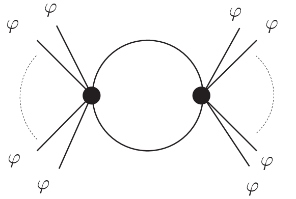
Figure 1: The graphical representation of the term explicitly shown in Eq.(LABEL:zeroK), the contribution to the effective action to the zeroth order in $K$, starting with $\varphi^{4}$. The blob stands for the vertex $G_{0,ij}$, which contains an even number of $\varphi$’s.

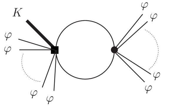
Figure 2: The graphical representation of the second term explicitly shown in Eq.(70), the contribution to the effective action to the first order in $K$, starting with $\varphi^{2}$. The blob stands for the vertex $G_{0,ij}$, which contains an even number of $\varphi$, and the square for the vertex $G_{1,ji}$, which contains a single $K$ as well as zero or an even number of $\varphi$’s.

A straightforward calculation gives the following expression for the first term,

$$-\frac{\bar{\varepsilon}^{-1}}{16F^{4}(4\pi)^{2}}\!\int\!\left[\prod_{i=1}^{4}\frac{d^{4}p_{i}}{(2\pi)^{4}}\right]\!(2\pi)^{4}\delta^{4}\!\left(\sum_{i=1}^{4}p_{i}\!\right)\!\prod_{i=1}^{4}\varphi_{l_{i}}(p_{i})$$

$$\times\bigg{\{}d_{kij}d_{kl_{1}l_{2}}d_{gji}d_{gl_{3}l_{4}}(p_{1}^{2}+p_{2}^{2})(p_{3}^{2}+p_{4}^{2})\frac{\mathstrut}{}$$

$$\hskip 10.00002pt{}+2d_{kij}d_{kl_{1}l_{2}}(d_{gji}d_{gl_{3}l_{4}}\!\!-\!d_{gjl_{3}}d_{gil_{4}})(p_{1}^{2}+p_{2}^{2})(p_{3}\cdot p_{4})$$

$$\hskip 10.00002pt{}+2d_{gji}d_{gl_{3}l_{4}}(d_{kij}d_{kl_{1}l_{2}}\!\!-\!d_{kil_{1}}d_{kjl_{2}})(p_{3}^{2}+p_{4}^{2})(p_{1}\cdot p_{2})$$

$$\hskip 10.00002pt{}+4(d_{kij}d_{kl_{1}l_{2}}-d_{kil_{1}}d_{kjl_{2}})(d_{gji}d_{gl_{3}l_{4}}-d_{gjl_{3}}d_{gil_{4}})$$

$$\hskip 20.00003pt{}\times(p_{1}\cdot p_{2})(p_{3}\cdot p_{4})$$

$$\hskip 10.00002pt-\frac{4}{3}d_{kil_{1}}d_{kjl_{2}}d_{gjl_{3}}d_{gil_{4}}$$

$$\hskip 20.00003pt{}\times\left[(p_{1}\cdot p_{4})(p_{2}\cdot p_{3})-(p_{1}\cdot p_{3})(p_{2}\cdot p_{4})\right]\bigg{\}}$$

$$+\text{(finite terms)}\;,$$ (60)

where $\bar{\varepsilon}^{-1}\equiv\varepsilon^{-1}-\gamma+\ln 4\pi$.

The next task is to separate the contributions which can be cancelled by symmetric counterterms from those which cannot be. The symmetric terms are already contained in the Lagrangian $\mathcal{L}[\phi]$ in Eq. (24), so that the addition of the counterterms is absorbed by the change of the coefficients of these operators. We list all of those terms up to including $\mathcal{O}(p^{4})$ that are invariant under axial-vector transformations. There are six independent ones;

$$\mathcal{L}_{1} = c_{1}\mathop{\rm tr}\nolimits\left(\Box U^{\dagger}\Box U\right),$$ (61)

$$\mathcal{L}_{2} = c_{2}\mathop{\rm tr}\nolimits\left(\partial_{\mu}U^{\dagger}\partial_{\mu}U\partial_{\nu}U^{\dagger}\partial_{\nu}U\right),$$ (62)

$$\mathcal{L}_{3} = c_{3}\mathop{\rm tr}\nolimits\left(\partial_{\mu}U^{\dagger}\partial_{\nu}U\partial_{\mu}U^{\dagger}\partial_{\nu}U\right),$$ (63)

$$\mathcal{L}_{4} = c_{4}\mathop{\rm tr}\nolimits\left(\partial_{\mu}U^{\dagger}\partial_{\mu}U\right)\left(\partial_{\nu}U^{\dagger}\partial_{\nu}U\right),$$ (64)

$$\mathcal{L}_{5} = c_{5}\mathop{\rm tr}\nolimits\left(\partial_{\mu}U^{\dagger}\partial_{\nu}U\right)\left(\partial_{\mu}U^{\dagger}\partial_{\nu}U\right),$$ (65)

$$\mathcal{L}_{6} = c_{6}\big{[}\mathop{\rm tr}\nolimits(\Box U^{\dagger}\partial_{\mu}U)\mathop{\rm tr}\nolimits(\partial_{\mu}U^{\dagger}U)$$ (66)

$$\hskip 20.00003pt{}+\mathop{\rm tr}\nolimits(U^{\dagger}\partial_{\mu}U)\mathop{\rm tr}\nolimits(\partial_{\mu}U^{\dagger}\Box U)\big{]}.$$

Expanding them in powers of $\phi$, and comparing the contributions to the effective action with those in Eq. (60) with the help of the formulae given in Appendix A, we see that we can cancel some of the divergences in Eq. (60) with the following values of $c_{i}$’s,

$$c_{1}=0, c_{2} =\frac{N}{48(4\pi)^{2}}\bar{\varepsilon}^{-1},$$

$$c_{3}=\frac{N}{96(4\pi)^{2}}\bar{\varepsilon}^{-1}, c_{4} =\frac{1}{32(4\pi)^{2}}\bar{\varepsilon}^{-1},$$

$$c_{5}=\frac{1}{16(4\pi)^{2}}\bar{\varepsilon}^{-1}, c_{6} =\frac{1}{16(4\pi)^{2}}\bar{\varepsilon}^{-1},$$ (67)

for the case of $\overline{MS}$ renormalization scheme. But, importantly, there are some divergences which cannot be canceled by the symmetric counterterms with any choice of the $c_{i}$’s. They are ANTs, which contribute to $B_{k}^{(\varphi^{3})}(p)$.

After adding the counterterms, we may define the apparently invariant (and finite) part of the effective action $\Gamma_{\mathrm{ITs}}^{(1)}[\varphi]$ of $\mathcal{O}(p^{4})$ coming from one-loop diagrams as

$$\Gamma_{\mathrm{ITs}}^{(1)}[\varphi]\! = \!-\frac{1}{4F^{4}(4\pi)^{2}}\int\left[\prod_{i=1}^{4}\frac{d^{4}p_{i}}{(2\pi)^{4}}\right](2\pi)^{4}\delta^{4}\left(\sum_{i=1}^{4}p_{i}\right)\prod_{i=1}^{4}\varphi_{l_{i}}(p_{i})$$ (68)

$$\times\left\{\left[2-\ln\frac{(p_{1}+p_{2})^{2}}{\mu^{2}}\right](d_{kij}d_{kl_{1}l_{2}}-d_{kil_{1}}d_{kjl_{2}})(d_{gji}d_{gl_{3}l_{4}}-d_{gjl_{3}}d_{gil_{4}})(p_{1}\cdot p_{2})(p_{3}\cdot p_{4})\frac{\mathstrut{}}{}\right.$$

$$\hskip 10.00002pt\left.-\frac{1}{3}\left[\frac{8}{3}-\ln\frac{(p_{1}+p_{2})^{2}}{\mu^{2}}\right]d_{kil_{1}}d_{kjl_{2}}d_{gjl_{3}}d_{gil_{4}}\left[(p_{1}\cdot p_{4})(p_{2}\cdot p_{3})-(p_{1}\cdot p_{3})(p_{2}\cdot p_{4})\right]\right\}+\mathcal{O}(\varphi^{6})\;.$$

The rest gives the apparently noninvariant (and infinite) part,

$$\Gamma_{\mathrm{ANTs}}^{(1)}[\varphi] = -\frac{1}{16F^{4}(4\pi)^{2}}\int\left[\prod_{i=1}^{4}\frac{d^{4}p_{i}}{(2\pi)^{4}}\right](2\pi)^{4}\delta^{4}\left(\sum_{i=1}^{4}p_{i}\right)\prod_{i=1}^{4}\varphi_{l_{i}}(p_{i})\left[\bar{\varepsilon}^{-1}+2-\ln\frac{(p_{1}+p_{2})^{2}}{\mu^{2}}\right]$$ (69)

$$\times\big{[}d_{kij}d_{kl_{1}l_{2}}d_{gji}d_{gl_{3}l_{4}}(p_{1}^{2}+p_{2}^{2})(p_{3}^{2}+p_{4}^{2})+2d_{kij}d_{kl_{1}l_{2}}(d_{gji}d_{gl_{3}l_{4}}-d_{gjl_{3}}d_{gil_{4}})(p_{1}^{2}+p_{2}^{2})(p_{3}\cdot p_{4})$$

$$+2d_{gji}d_{gl_{3}l_{4}}(d_{kij}d_{kl_{1}l_{2}}-d_{kil_{1}}d_{kjl_{2}})(p_{3}^{2}+p_{4}^{2})(p_{1}\cdot p_{2})\big{]}+\mathcal{O}(\varphi^{6})\;.$$

The $\mathcal{O}(\varphi^{4})$ terms contribute to $B_{k}^{(\varphi^{3})}$.

Similarly, we can calculate the $\mathcal{O}(\varphi^{2}K^{1})$ terms of the effective action $\Gamma^{(1)}[\varphi,K]$. At the first order in K, we have

$$\frac{1}{2}\ln\mathop{\rm Det}\nolimits[D_{F}^{-1}]|_{K^{1}}$$ (70)

$$= \!\!-\frac{1}{2}\!\int\!\frac{d^{d}k_{1}}{(2\pi)^{d}}\!\!\int\!\frac{d^{d}k_{2}}{(2\pi)^{d}}\frac{1}{k_{1}^{2}}G_{0,ij}(k_{1},\!-k_{2})\frac{1}{k_{2}^{2}}G_{1,ji}(k_{2},\!-k_{1})$$

$$+\mathcal{O}(\varphi^{4}K)\;.$$

We obtain for the second term

$$\frac{1}{4F^{3}(4\pi)^{2}}\int\!\frac{d^{4}p_{1}}{(2\pi)^{4}}\int\!\frac{d^{4}p_{2}}{(2\pi)^{4}}\int\!\frac{d^{4}p}{(2\pi)^{4}}$$

$$\times(2\pi)^{4}\delta^{4}(p_{1}+p_{2}+p)\varphi_{l_{1}}(p_{1})\varphi_{l_{2}}(p_{2})K_{k}(p)$$

$$\times\left(\bar{\varepsilon}^{-1}+2-\ln(p^{2}/\mu^{2})\right)$$

$$\times\left[d_{gij}d_{gl_{1}l_{2}}p^{2}-2d_{gil_{1}}d_{gjl_{2}}(p_{1}\cdot p_{2})\right]d_{kij}\;,$$ (71)

which contributes to $C_{j}^{(\varphi^{2})}$.

Now we are ready to calculate Eq. (53). Noting that we only need $B_{k}^{(\varphi^{3})}(p)$ at $p=0$ (because of the delta function in Eq. (54)) and that only the terms with $j=0$ survive (because of the $\delta_{0j}$) and $d_{i0k}$ is proportional to $\delta_{ik}$ simplifies the calculation. We finally obtain for the first term of Eq. (53)

$$d_{ijk}\int\!\frac{d^{d}p}{(2\pi)^{d}}\sigma_{j}^{(\varphi^{0})}(p)B_{k}^{(\varphi^{3})}(p)$$ (72)

$$= -\frac{1}{4F^{3}(4\pi)^{2}}\int\!\frac{d^{4}p_{1}}{(2\pi)^{4}}\int\!\frac{d^{4}p_{2}}{(2\pi)^{4}}\int\!\frac{d^{4}p_{3}}{(2\pi)^{4}}$$

$$\times(2\pi)^{4}\delta^{4}(p_{1}+p_{2}+p_{3})\varphi_{l_{1}}(p_{1})\varphi_{l_{2}}(p_{2})\varphi_{l_{3}}(p_{3})$$

$$\times\left(\bar{\varepsilon}^{-1}+2-\ln(p_{3}^{2}/\mu^{2})\right)d_{hnm}d_{hl_{3}i}$$

$$\times\left[d_{gmn}d_{gl_{1}l_{2}}p_{3}^{2}-d_{gml_{1}}d_{gnl_{2}}(p_{1}\cdot p_{2})\right]p_{3}^{2}\;.$$

The calculation of the second term of Eq. (53) is simpler and one easily finds that it is the same as Eq. (72) but with the opposite sign. Thus we have explicitly demonstrated that Eq. (48) is satisfied in $\mathcal{O}(\varphi^{3})$.

We have shown that the one-loop effective action $\Gamma^{(1)}[\varphi]$ is not invariant under the naive axial-vector transformation. But it does satisfy the WT identity so that the symmetry is preserved.

IV Divergent part of $\Gamma_{\mathrm{ANTs}}^{(1)}[\varphi]$ to all order in $\varphi$

In the previous section, by expanding $\Gamma[\varphi,K]$ in powers of $\varphi$ up to including $\mathcal{O}(\varphi^{4})$ and $\mathcal{O}(\varphi^{2}K^{1})$, we obtain $\Gamma_{\mathrm{ANTs}}^{(1)}[\varphi]$ to $\mathcal{O}(\varphi^{4})$. But the invariance expressed by the Zinn-Justin equation is actually more powerful; it determines the form of the divergent part (i.e., the part that is proportional to $\bar{\varepsilon}^{-1}$) of $\Gamma_{\mathrm{ANTs}}^{(1)}[\varphi]$ to all order of $\varphi$. The following construction originally appears in Ref. Brezin et al. (1976). It is similar to the analysis done by Ferrari and Quadri Ferrari and Quadri (2006a) for the case of $SU(2)\times SU(2)$.

Let us return to Eq. (38). It can be written as

$$s_{i}\Gamma^{(1)}[\varphi,K]=0\;,$$ (73)

by introducing a differential operator $s_{i}$,

$$s_{i}\equiv d_{ijk}\int d^{d}x\left(\sigma_{j}(x)\frac{\delta}{\delta\varphi_{k}(x)}-H_{k}(x)\frac{\delta}{\delta K_{j}(x)}\right)\;,$$ (74)

where $H_{k}$ is defined as

$$H_{k}(x)\equiv-\frac{\delta S[\varphi,K]}{\delta\varphi_{k}(x)}=-\frac{\delta S[\varphi]}{\delta\varphi_{k}(x)}-\int\!d^{d}y\frac{\partial\sigma_{i}(y)}{\partial\varphi_{k}(x)}K_{i}(y)\;.$$ (75)

Since $\Gamma_{\mathrm{ITs}}^{(1)}[\varphi]$ satisfies

$$s_{i}\Gamma_{\mathrm{ITs}}^{(1)}[\varphi]=0\;,$$ (76)

we have

$$s_{i}\left(\Gamma_{\mathrm{ANTs}}^{(1)}[\varphi]+\hat{\Gamma}^{(1)}[\varphi,K]\right)=0\;.$$ (77)

In the following, we discuss only the divergent parts, that is, the local functionals of $\varphi$ and $K$.

An important observation is that $K$ and $H$ transform in the same way as $\sigma$ and $\varphi$ do :

$$\left\{\begin{array}[]{l}s_{i}K_{j}=-d_{ijk}H_{k}\;,\\ s_{i}H_{j}=d_{ijk}K_{k}\;,\end{array}\right.$$ (78)

$$\left\{\begin{array}[]{l}s_{i}\sigma_{j}=-d_{ijk}\varphi_{k}\;,\\ s_{i}\varphi_{j}=d_{ijk}\sigma_{k}\;.\end{array}\right.$$ (79)

Invariants are most easily formed in terms of $U=(\sigma+i\varphi)/F$. In the same way, we introduce

$$L=\frac{1}{F}\left(K+iH\right)=\frac{2}{F}\left(K_{i}+iH_{i}\right)T_{i}\;,$$ (80)

and form invariants in terms of $U$ and $L$. Note that $L$ has the same property under parity as that of $U$.

We remark that the divergence of the effective action occurs in the terms at most quadratic in $K$ in the one-loop approximation. To represent them, therefore, we only consider the invariants at most quadratic in $L$. We also remark that the vertices containing $K$ do not involve derivatives, thus the divergent part of the effective action quadratic in $L$ does not involves derivatives, either.

There are five independent invariants contributing to $\Gamma_{\mathrm{ANTs}}^{(1)}[\varphi]+\hat{\Gamma}^{(1)}[\varphi,K]$ up to including $\mathcal{O}(p^{4})$ and $\mathcal{O}(\varphi^{4})$ when expanded and consisting of $U$ and $L$,

$$O_{1} = \mathop{\rm tr}\nolimits(L^{{\dagger}}L),$$ (81)

$$O_{2} = \frac{1}{4}\left[\mathop{\rm tr}\nolimits(U^{{\dagger}}L)+\mathop{\rm tr}\nolimits(L^{{\dagger}}U)\right]^{2},$$ (82)

$$O_{3} = \frac{1}{2}\left[\mathop{\rm tr}\nolimits(\Box U^{{\dagger}}L)+\mathop{\rm tr}\nolimits(L^{{\dagger}}\Box U)\right],$$ (83)

$$O_{4} = \frac{1}{2}\mathop{\rm tr}\nolimits(\partial_{\mu}U^{{\dagger}}\partial_{\mu}U)\left[\mathop{\rm tr}\nolimits(U^{{\dagger}}L)+\mathop{\rm tr}\nolimits(L^{{\dagger}}U)\right],$$ (84)

$$O_{5} = \frac{1}{4}\left[\mathop{\rm tr}\nolimits(U^{{\dagger}}\partial_{\mu}U)-\mathop{\rm tr}\nolimits(\partial_{\mu}U^{{\dagger}}U)\right]$$ (85)

$$\hskip 10.00002pt\times{}\left[\mathop{\rm tr}\nolimits(\partial_{\mu}U^{{\dagger}}L)-\mathop{\rm tr}\nolimits(L^{{\dagger}}\partial_{\mu}U)\right],$$

besides the ones consisting only of $U$ listed in Eqs. (61) – (66).

One might think that there should be more invariants which start with $\varphi^{6}$ when expanded, but because of the constraint $U^{\dagger}U=I$, such an invariant requires at least six derivatives; there is no other invariant than $O_{i}\ (i=1,\cdots,5)$ to this order. Thus $\Gamma_{\mathrm{ANTs}}^{(1)}[\varphi]+\hat{\Gamma}^{(1)}[\varphi,K]$ can be expressed as a linear combination of the integrals of these invariants.

By comparing the $\mathcal{O}(\varphi^{4})$ and $\mathcal{O}(\varphi^{2}K)$ terms with Eqs. (69) and (70), we can determine the coefficients. We can determine the divergent part of $\Gamma_{\mathrm{ANTs}}^{(1)}[\varphi]+\hat{\Gamma}^{(1)}[\varphi,K]$ to all order in $\varphi$ as,

$$\left(\Gamma_{\mathrm{ANTs}}^{(1)}[\varphi]+\hat{\Gamma}^{(1)}[\varphi,K]\right)_{\mbox{\scriptsize div}}$$

$$= -\frac{\bar{\varepsilon}^{-1}}{8(4\pi)^{2}}\int\!d^{d}x\left[N(O_{1}-O_{3})+O_{2}+O_{4}-2O_{5}\right].$$

(86)

By setting $K=0$, we see that $L$ is then proportional to $\delta S/\delta\varphi$,

$$L\rightarrow-\frac{2i}{F}\frac{\delta S}{\delta\varphi_{i}}T_{i}\;.$$ (87)

We therefore see that the divergent part of $\Gamma_{\mathrm{ANTs}}^{(1)}[\varphi]$ is proportional to $\delta S/\delta\varphi$.

It is well known ’t Hooft (1973) that the part of the one-loop effective action that is proportional to $\delta S/\delta\varphi$ does not contribute to the S-matrix elements, due to the “equivalence theorem Kamefuchi et al. (1961)” That is, ANTs of the amputated connected Green function (ACGF) vanish on shell.

V Six-point functions

There seems to be a little confusion about the “use of the equations of motion,” $\delta S/\delta\varphi=0$, and the “on-shell condition,” $p_{i}^{2}=0$. Some authors use them interchangeably. But they are essentially different. ANTs of the one-loop effective action vanish by the use of the equations of motion.

One might think that it implies that the ANTs contained in the $n$-point proper vertices generated by the effective action also vanish on shell. But this is not the case.

It is not the $n$-point proper vertices, but the ACGF whose ANTs vanish on shell, because of the equivalence theorem.

For the four-point functions, however, the difference is not seen; the proper vertex coincides with the ACGF in the one-loop approximation. Thus ANTs of the proper vertex happen to vanish on shell. See Eq. (69).

It is therefore interesting to examine the six-point functions because the difference between the ACGF and the proper vertex first appears in the six-point functions at the one-loop order. Since we have obtained the divergent part of the one-loop effective action to all order in $\varphi$, we are ready to examine the $n$-point functions with $n\geq 6$.

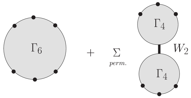
Figure 3: The graphical representation of the right hand side of Eq. (93). A solid circle stands an amputated external line and the solid line for the full propagator, $W_{\rho\sigma}$, abbreviated as $W_{2}$. The gray blobs stand for the proper vertices. $\Gamma_{6}$ is the abbreviated notation for $\Gamma_{\alpha_{1}\cdots\alpha_{6}}$, and $\Gamma_{4}$ for $\Gamma_{\alpha_{i_{1}}\alpha_{i_{2}}\alpha_{i_{3}}\rho}$ and $\Gamma_{\alpha_{i_{4}}\alpha_{i_{5}}\alpha_{i_{6}}\rho}$. The sum is taken over the permutation of the external lines.

We first show that the ANTs of the six-point proper vertex do not vanish on shell. Because we are interested in the proper vertices in the absence of $K$, we set $K=0$. By expanding $O_{i}\ (i=1,\cdots,5)$ in terms of $\varphi$, we see that the contributions from $O_{2}$, $O_{3}$ vanish on shell. The $O(\varphi^{6})$ part of $O_{1}$ is given by

$$\frac{1}{F^{4}}d_{gji_{1}}d_{gi_{2}i_{3}}d_{hji_{4}}d_{hi_{5}i_{6}}\varphi_{i_{1}}\varphi_{i_{4}}\partial_{\mu}\varphi_{i_{2}}\partial_{\mu}\varphi_{i_{3}}\partial_{\nu}\varphi_{i_{5}}\partial_{\nu}\varphi_{i_{6}},$$ (88)

up to the terms proportional to $\Box\varphi_{i}$, which vanish on shell. Similarly, from $O_{4}$ and $O_{5}$, we have the contributions that do not vanish on shell,

$$\frac{1}{F^{2}}d_{ijk}d_{ilm}\varphi_{j}\varphi_{k}\partial_{\mu}\varphi_{l}\partial_{\mu}\varphi_{m}(\partial_{\nu}\varphi_{g})^{2},$$ (89)

$$\frac{1}{F^{2}}\sqrt{\frac{N}{2}}d_{i,jk,lm}\varphi_{j}\partial_{\mu}\varphi_{k}\varphi_{i}\partial_{\nu}\varphi_{l}\partial_{\nu}\varphi_{m}\partial_{\mu}\varphi_{0},$$

respectively, where $d_{i,jk,lm}$ stands for $d_{igh}d_{gjk}d_{hlm}$. Substituting these contributions in Eq. (86), we see that the divergent part of $\Gamma_{\mathrm{ANTs}}^{(1)}[\varphi]$ contains

$$-\frac{\bar{\varepsilon}^{-1}}{8F^{6}(4\pi)^{2}}\int\left[\prod_{i=1}^{6}\frac{d^{4}p_{i}}{(2\pi)^{4}}\right]\!\!(2\pi)^{4}\delta^{4}\!\left(\sum_{i=1}^{6}p_{i}\!\right)\prod_{k=1}^{6}\varphi_{i_{k}}(p_{k})$$

$$\times d_{i_{1}i_{2},i_{3}i_{4},i_{5}i_{6}}(p_{1}\cdot p_{2})(p_{3}\cdot p_{4})$$ (91)

that gives rise to the nonvanishing contribution to the six-point proper vertex. Here we have introduced another notation,

$$d_{i_{1}i_{2},i_{3}i_{4},i_{5}i_{6}}$$ (92)

$$= Nd_{gi_{1}i_{2}}d_{hi_{3}i_{4}}(d_{gki_{5}}d_{hki_{6}}+d_{gki_{5}}d_{hki_{6}})$$

$${}+2d_{ki_{5}i_{6}}(d_{ki_{1}i_{2}}\delta_{i_{3}i_{4}}+d_{ki_{3}i_{4}}\delta_{i_{1}i_{2}})$$

$$-\sqrt{\frac{N}{2}}\big{[}(d_{i_{5},i_{1}i_{2},i_{4}i_{6}}+d_{i_{6},i_{1}i_{2},i_{4}i_{5}})\delta_{i_{3}0}$$

$$\hskip 30.00005pt+(d_{i_{5},i_{1}i_{2},i_{3}i_{6}}+d_{i_{6},i_{1}i_{2},i_{3}i_{5}})\delta_{i_{4}0}$$

$$\hskip 30.00005pt+(d_{i_{5},i_{3}i_{4},i_{2}i_{6}}+d_{i_{6},i_{3}i_{4},i_{2}i_{5}})\delta_{i_{1}0}$$

$$\hskip 30.00005pt+(d_{i_{5},i_{3}i_{4},i_{1}i_{6}}+d_{i_{6},i_{3}i_{4},i_{1}i_{5}})\delta_{i_{2}0}\big{]}.$$

Thus, we have established that the divergent part of ANTs in the six-point proper vertex does not vanish on shell.

We will show that ANTs contained in the six-point ACGF do vanish on shell. In an abbreviated notation, the six-point ACGF is written as

$$\Gamma_{\alpha_{1}\beta_{1}}\Gamma_{\alpha_{2}\beta_{2}}\Gamma_{\alpha_{3}\beta_{3}}\Gamma_{\alpha_{4}\beta_{4}}\Gamma_{\alpha_{5}\beta_{5}}\Gamma_{\alpha_{6}\beta_{6}}W_{\beta_{1}\beta_{2}\beta_{3}\beta_{4}\beta_{5}\beta_{6}}$$ (93)

$$= \Gamma_{\alpha_{1}\alpha_{2}\alpha_{3}\alpha_{4}\alpha_{5}\alpha_{6}}$$

$$+\left(\Gamma_{\alpha_{1}\alpha_{2}\alpha_{3}\rho}\Gamma_{\alpha_{4}\alpha_{5}\alpha_{6}\sigma}+\mbox{9 similar terms}\right)W_{\rho\sigma},$$

where $W_{\alpha_{1}\alpha_{2}\cdots\alpha_{n}}$ is a connected Green function,

$$W_{\alpha_{1}\alpha_{2}\cdots\alpha_{n}}\equiv(-1)^{n}\left.\frac{\delta^{n}W[J]}{\delta J_{\alpha_{1}}\cdots\delta J_{\alpha_{n}}}\right|_{J=0},$$ (94)

where $W[J]=W[J,K=0]$ and $\Gamma_{\alpha_{1}\alpha_{2}\cdots\alpha_{n}}$ is a proper vertex,

$$\Gamma_{\alpha_{1}\alpha_{2}\cdots\alpha_{n}}\equiv\left.\frac{\delta^{n}\Gamma[\varphi]}{\delta\varphi_{\alpha_{1}}\cdots\delta\varphi_{\alpha_{n}}}\right|_{\varphi=0}.$$ (95)

Note that because the invariant terms are made finite by the addition of the invariant counterterms, the divergent parts of the both sides of Eq. (93) come only from ANTs.

The assertion is that, despite the nonvanishing divergent part of ANTs in one-loop contributions to the first term in Eq. (93) on shell, the sum does not contain such ANTs. Note that the tree contributions of course do not contain ANTs.

In the one-loop approximation, the propagator $W_{\rho\sigma}$ is the free one thanks to a property of dimensional regularization. In the product $\Gamma_{\alpha_{1}\alpha_{2}\alpha_{3}\rho}\Gamma_{\alpha_{4}\alpha_{5}\alpha_{6}\sigma}$ one of the two $\Gamma$’s must be the one-loop contribution while the other must be the tree one. Thus the noninvariant divergent contributions to the $\Gamma_{\alpha_{1}\alpha_{2}\alpha_{3}\rho}\Gamma_{\alpha_{4}\alpha_{5}\alpha_{6}\sigma}W_{\rho\sigma}$ in the one-loop approximation contain the following divergent part,

$$\int\!\frac{d^{d}p}{(2\pi)^{d}}\int\!\frac{d^{d}k}{(2\pi)^{d}}\bigg{[}(2\pi)^{4d}\frac{\delta^{4}S[\varphi]}{\delta\varphi_{i_{1}}(q_{1})\delta\varphi_{i_{2}}(q_{2})\delta\varphi_{i_{3}}(q_{3})\delta\varphi_{j}(p)}(2\pi)^{4d}\frac{\delta^{4}\left(\Gamma_{\mathrm{ANTs}}^{(1)}[\varphi]\right)_{\mbox{\scriptsize div.}}}{\delta\varphi_{i_{4}}(q_{4})\delta\varphi_{i_{5}}(q_{5})\delta\varphi_{i_{6}}(q_{6})\delta\varphi_{k}(k)}$$ (96)

$$\hskip 30.00005pt+(2\pi)^{4d}\frac{\delta^{4}\left(\Gamma_{\mathrm{ANTs}}^{(1)}[\varphi]\right)_{\mbox{\scriptsize div.}}}{\delta\varphi_{i_{1}}(q_{1})\delta\varphi_{i_{2}}(q_{2})\delta\varphi_{i_{3}}(q_{3})\delta\varphi_{j}(p)}(2\pi)^{4d}\frac{\delta^{4}S[\varphi]}{\delta\varphi_{i_{4}}(q_{4})\delta\varphi_{i_{5}}(q_{5})\delta\varphi_{i_{6}}(q_{6})\delta\varphi_{k}(k)}\bigg{]}_{\varphi=0}\frac{-1}{k^{2}}(2\pi)^{d}\delta^{d}(k+p)\delta_{jk}$$

$$= \frac{2\bar{\varepsilon}^{-1}}{F^{6}(4\pi)^{2}}(2\pi)^{d}\delta^{d}\left(\sum_{i=1}^{6}q_{i}\right)\bigg{[}d_{i_{1}i_{2}i_{3},i_{4}i_{5}i_{6}}(q_{1}\cdot q_{2})(q_{4}\cdot q_{5})+d_{i_{1}i_{2}i_{3},i_{4}i_{6}i_{5}}(q_{1}\cdot q_{2})(q_{4}\cdot q_{6})+d_{i_{1}i_{2}i_{3},i_{5}i_{6}i_{4}}(q_{1}\cdot q_{2})(q_{5}\cdot q_{6})$$

$$\hskip 30.00005pt+d_{i_{1}i_{3}i_{2},i_{4}i_{5}i_{6}}(q_{1}\cdot q_{3})(q_{4}\cdot q_{5})+d_{i_{1}i_{3}i_{2},i_{4}i_{6}i_{5}}(q_{1}\cdot q_{3})(q_{4}\cdot q_{6})+d_{i_{1}i_{3}i_{2},i_{5}i_{6}i_{4}}(q_{1}\cdot q_{3})(q_{5}\cdot q_{6})$$

$$\hskip 30.00005pt+d_{i_{2}i_{3}i_{1},i_{4}i_{5}i_{6}}(q_{2}\cdot q_{3})(q_{4}\cdot q_{5})+d_{i_{2}i_{3}i_{1},i_{4}i_{6}i_{5}}(q_{2}\cdot q_{3})(q_{4}\cdot q_{6})+d_{i_{2}i_{3}i_{1},i_{5}i_{6}i_{4}}(q_{2}\cdot q_{3})(q_{5}\cdot q_{6})\bigg{]}$$

$${}+(\mbox{terms those do not contribute on shell}),$$

where we introduce

$$d_{i_{1}i_{2}i_{3},i_{4}i_{5}i_{6}}$$ (97)

$$\equiv d_{gij}d_{li_{1}i_{2}}d_{i_{3}lk}(d_{hij}d_{hi_{4}i_{5}}-d_{hii_{4}}d_{hji_{5}})d_{i_{6}gk}$$

$${}+(i_{1}i_{2}i_{3}\leftrightarrow i_{4}i_{5}i_{6}).$$

Note that, with the help of the formulae given in Appendix B, one can show that

$$d_{i_{1}i_{2},i_{3}i_{4},i_{5}i_{6}} = d_{i_{1}i_{2}i_{5},i_{3}i_{4}i_{6}}+d_{i_{1}i_{2}i_{6},i_{3}i_{4}i_{5}}\;,$$ (98)

which is useful in the following demonstration.

In a similar way, we can calculate all the divergent terms contained in

$$\left(\Gamma_{\alpha_{1}\alpha_{2}\alpha_{3}\rho}\Gamma_{\alpha_{4}\alpha_{5}\alpha_{6}\sigma}+\mbox{9 similar terms}\right)W_{\rho\sigma}$$ (99)

at one-loop that do not vanish on shell. There are 90 similar terms to

$$\frac{2\bar{\varepsilon}^{-1}}{F^{6}(4\pi)^{2}}d_{i_{1}i_{2}i_{3},i_{4}i_{5}i_{6}}(q_{1}\cdot q_{2})(q_{4}\cdot q_{5}).$$ (100)

On the other hand, the differentiation of Eq. (91) with respect to $\varphi$ six times produces $6!=720$ terms but every 16 ($=2^{4}$) terms are actually identical. (Note the symmetry under the interchange of the indices, $i_{1}\leftrightarrow i_{2}$, $i_{3}\leftrightarrow i_{4}$, $i_{5}\leftrightarrow i_{6}$, and $(i_{1}i_{2})\leftrightarrow(i_{3}i_{4})$ of the representative term $d_{i_{1}i_{2},i_{3}i_{4},i_{5}i_{6}}(p_{1}\cdot p_{2})(p_{3}\cdot p_{4})$.) Thus we have 45 ($=720/16$) similar terms to

$$-\frac{2\bar{\varepsilon}^{-1}}{F^{6}(4\pi)^{2}}d_{i_{1}i_{2},i_{3}i_{4},i_{5}i_{6}}(q_{1}\cdot q_{2})(q_{3}\cdot q_{4}).$$ (101)

Now substituting Eq. (98), we see that the divergent terms in the first term of the right hand side of Eq. (93) is exactly equal to those in the second term with the opposite sign. Thus we have shown that the divergent terms cancel in the ACGF on shell.

VI Summary

In this paper, we have explained why ANTs emerge in theories with nonlinearly realized symmetry. The naive variation of the classical field $\varphi$ under the symmetry is in general not equal to the expectation value of the variation of the quantum field $\phi$, so that the effective action $\Gamma[\varphi]$ is not invariant under the naive variation of $\varphi$. In this respect, the emergence of ANTs is not limited to NLSMs.

We have formulate the WT identity as an inhomogeneous Zinn-Justin equation for the $U(N)\times U(N)$ NLSMs to investigated the nature of ANTs. We have shown that ANTs are consistent with the symmetry.

An explicit one-loop calculation is presented for the four-point functions. We then determine the divergent part of the ANTs in the one-loop effective action, $\Gamma_{\mathrm{ANTs}}^{(1)}[\varphi]$, to all order in $\varphi$.

It is shown that the divergent part of the ANTs in the six-point proper vertex does not vanish when the external momenta are all set to be on shell, in contrast to the four-point proper vertex, whose divergent part of the ANTs vanishes on shell. We have shown that, despite its presence in the proper vertices, ANTs contained in the six-point ACGF do vanish on shell. We believe that higher-point ACGF also have this property.

Note that we do not subtract divergences in $\Gamma_{\mathrm{ANTs}}^{(1)}[\varphi]$; the introduction of noninvariant counterterms cause the violation of the original symmetry. Even though they are divergent, ANTs do not contribute to the S-matrix elements after all. It provides an example where the effective action is divergent while the S-matrix elements are finite.

We expect that similar properties hold even in higher order in the loop-wise expansion.

Appendix A Some useful formulae for $U(N)$

In this Appendix, we summarize some formulae for the symmetric tensor $d_{ijk}$, which are used in the loop calculations. See Refs. MacFarlane et al. (1968); Geddes (1979) for the details.

We consider the $U(N)$ generators as $N\times N$ matrices, $T_{i}\ (i=0,1,\cdots,N^{2}-1)$, satisfying the relations in Eqs. (11), (12), and (13).

By considering the Jacobi identities,

$${}[[T_{i},T_{j}],T_{k}]+[[T_{j},T_{k}],T_{i}]+[[T_{k},T_{i}],T_{j}]=0,$$ (102)

$${}[\{T_{i},T_{j}\},T_{k}]+[\{T_{j},T_{k}\},T_{i}]+[\{T_{k},T_{i}\},T_{j}]=0,\qquad$$ (103)

$${}[T_{k},[T_{i},T_{j}]]=\{T_{j},\{T_{k},T_{i}\}\}-\{T_{i},\{T_{j},T_{k}\}\},$$ (104)

we find the following relations between $f_{ijk}$’s and $d_{ijk}$’s,

$$f_{ilm}f_{mjk}+f_{jlm}f_{imk}+f_{klm}f_{ijm}=0,$$ (105)

$$f_{ilm}d_{mjk}+f_{jlm}d_{imk}+f_{klm}d_{ijm}=0,$$ (106)

$$f_{ijm}f_{klm}-d_{ikm}d_{jlm}+d_{jkm}d_{ilm}=0.$$ (107)

From them one can derive useful relations.

Let us introduce $N^{2}\times N^{2}$ matrices, $(D_{j})_{ik}$,

$$(D_{j})_{ik}\equiv d_{ijk},$$ (108)

which satisfy

$$\mathop{\rm tr}\nolimits(D_{i}D_{j}) = N(\delta_{ij}+\delta_{i0}\delta_{j0}),$$ (109)

$$\mathop{\rm tr}\nolimits(D_{i}D_{j}D_{k}) = \frac{N}{2}d_{ijk}+\sqrt{\frac{N}{2}}(\delta_{i0}\delta_{jk}+\delta_{j0}\delta_{ik}$$ (110)

$$\hskip 60.00009pt+\delta_{k0}\delta_{ij}),$$

$$\mathop{\rm tr}\nolimits(D_{i}D_{j}D_{k}D_{l}) = \frac{N}{4}(d_{ijm}d_{mkl}-f_{ijm}f_{mkl})$$ (111)

$${}+\frac{1}{2}(\delta_{ij}\delta_{kl}+\delta_{ik}\delta_{jl}+\delta_{il}\delta_{jk})$$

$$+\frac{\sqrt{2N}}{4}(\delta_{i0}d_{jkl}+\delta_{j0}d_{ikl}+\delta_{k0}d_{ijl}$$

$${}\hskip 40.00006pt+\delta_{l0}d_{ijk}).$$

They are used in reducing the result of Eq. (60) in a compact form for the comparison with the local terms listed in Eqs.(61) through (66).

Appendix B $SU(2)\times SU(2)$ case

In this Appendix, we present the results for the $SU(2)\times SU(2)$ case. Because of the extra $U(1)$ factors, the $SU(2)\times SU(2)$ results cannot be obtained directly from those for $U(N)\times U(N)$. The purpose of this Appendix is to provide a useful reference for those who are familiar with the literature devoted to the $SU(2)\times SU(2)$ case.

For the $SU(2)\times SU(2)$ case, the most useful parameterization is given by Eq. (2). (But we continue to use the notation $\phi^{a}$ instead of $\pi^{a}$.) We consider the generating functional,

$$e^{-W[J,K]}\!=\!\int\!\mathcal{D}\phi\;\exp\left[-\!\int\!d^{4}x\left(\mathcal{L}+\sigma K\right)\!+\!\int\!d^{4}x\phi_{a}J_{a}\right],$$ (112)

and define the effective action as usual. The inhomogeneous Zinn-Justin equation is given by

$$\int d^{4}x\left(\frac{\delta\Gamma[\varphi,K]}{\delta K(x)}\frac{\delta\Gamma[\varphi,K]}{\delta\varphi_{a}(x)}+\varphi_{a}(x)K(x)\right)=0.$$ (113)

The one-loop calculation for the effective action, $\Gamma^{(1)}[\varphi,K]$, can be done in a similar way, but the results are much simpler. The $K$-independent part contains

$$-\frac{\bar{\varepsilon}^{-1}}{16F^{4}(4\pi)^{2}}\!\int\!\left[\prod_{i=1}^{4}\frac{d^{4}p_{i}}{(2\pi)^{4}}\right]\!(2\pi)^{4}\delta^{4}\!\left(\sum_{i=1}^{4}p_{i}\!\right)$$

$${}\times\varphi_{a}(p_{1})\varphi_{a}(p_{2})\varphi_{b}(p_{3})\varphi_{b}(p_{4})$$

$${}\times\bigg{[}3(p_{1}^{2}+p_{2}^{2})(p_{3}^{2}+p_{4}^{2})+4(p_{1}^{2}+p_{2}^{2})(p_{3}\cdot p_{4})$$

$$\hskip 10.00002pt{}+4(p_{3}^{2}+p_{4}^{2})(p_{1}\cdot p_{2})+\frac{8}{3}(p_{1}\cdot p_{2})(p_{3}\cdot p_{4})$$

$$\hskip 10.00002pt{}+\frac{8}{3}(p_{1}\cdot p_{4})(p_{2}\cdot p_{3})+\frac{8}{3}(p_{1}\cdot p_{3})(p_{2}\cdot p_{4})\bigg{]}$$

$$\hskip 10.00002pt{}+\text{(finite terms)},$$ (114)

instead of Eq. (60). There are only three independent symmetric counterterms of this order because of the relations,

$$\mathop{\rm tr}\nolimits(\partial_{\mu}U^{{\dagger}}\partial_{\mu}U\partial_{\nu}U^{{\dagger}}\partial_{\nu}U) = \frac{1}{2}[\mathop{\rm tr}\nolimits(\partial_{\mu}U^{{\dagger}}\partial_{\mu}U)]^{2},$$ (115)

$$\mathop{\rm tr}\nolimits(\partial_{\mu}U^{{\dagger}}\partial_{\nu}U\partial_{\mu}U^{{\dagger}}\partial_{\nu}U) = [\mathop{\rm tr}\nolimits(\partial_{\mu}U^{{\dagger}}\partial_{\nu}U)]^{2}$$ (116)

$${}-\frac{1}{2}[\mathop{\rm tr}\nolimits(\partial_{\mu}U^{{\dagger}}\partial_{\mu}U)]^{2},\ \$$

which hold for the $SU(2)$ case, and

$$\mathop{\rm tr}\nolimits(U^{\dagger}\partial_{\mu}U)=\mathop{\rm tr}\nolimits(\partial_{\mu}U^{\dagger}U)=0,$$ (117)

due to the tracelessness of the generators. Thus there are only three independent invariants, $\mathcal{L}_{1}$, $\mathcal{L}_{4}$, and $\mathcal{L}_{5}$. By expanding $\mathcal{L}_{i}\ (i=1,4,5)$ in $\varphi$ and comparing the momentum dependence of them with the terms in Eq. (114), we see that some of the divergences can be removed by these counterterms with the coefficients,

$$c_{1}=0,\quad c_{4}=\frac{1}{24(4\pi)^{2}}\bar{\varepsilon}^{-1},\quad c_{5}=\frac{1}{12(4\pi)^{2}}\bar{\varepsilon}^{-1},$$ (118)

which agree with the result Eq. (3.4) of Ref. Appelquist and Bernard (1981). (Note that there is a factor 2 difference coming from the difference between their $\epsilon=4-d$ and our $\varepsilon=(4-d)/2$, and the difference of signs coming from that we are working in Euclidean space.)

Similarly, for the linear part in $K$, we have

$$\frac{1}{4F^{3}(4\pi)^{2}}\int\!\frac{d^{4}p_{1}}{(2\pi)^{4}}\int\!\frac{d^{4}p_{2}}{(2\pi)^{4}}\int\!\frac{d^{4}p}{(2\pi)^{4}}$$

$$\times(2\pi)^{4}\delta^{4}(p_{1}+p_{2}+p)\varphi_{a}(p_{1})\varphi_{a}(p_{2})K(p)$$

$$\times(\bar{\varepsilon}^{-1}+2-\ln(p^{2}/\mu^{2}))\left[3p^{2}-2(p_{1}\cdot p_{2})\right],$$ (119)

instead of Eq. (71). The divergent part of $\Gamma_{\mathrm{ANTs}}^{(1)}[\varphi]+\hat{\Gamma}^{(1)}[\varphi,K]$ up to including $\mathcal{O}(p^{4})$ may be written as a linear combination of $O_{i}$’s listed in Eqs. (81) – (85), where $L$ is now defined as

$$L=\frac{1}{F}\left[K+i\vec{\tau}\cdot\vec{H}\right],$$ (120)

where

$$H_{a}\equiv-\frac{\delta S[\varphi]}{\delta\varphi_{a}}+\frac{\varphi_{a}}{\sigma}K,$$ (121)

instead of Eq. (80).

Because of the difference between $U(N)$ and $SU(2)$, however, not all of $O_{i}$’s are independent in the case of $SU(2)$. First of all, $O_{5}$ vanishes because of Eq. (117). There are also relations among the rest.

Consider $O_{1}$ and $O_{2}$ for example. Using (121), we can rewrite them as

$$O_{1} = \frac{2}{F^{2}}\left[\frac{F^{2}K^{2}}{\sigma^{2}}-2\frac{K}{\sigma}\varphi_{a}S_{a}+S_{a}^{2}\right],$$ (122)

$$O_{2} = \frac{4}{F^{4}}\left[\frac{F^{4}K^{2}}{\sigma^{2}}-2\frac{F^{2}K}{\sigma}\varphi_{a}S_{a}+\left(\varphi_{a}S_{a}\right)^{2}\right],\ \$$ (123)

where we have introduced the notation $S_{a}\equiv\delta S[\varphi]/\delta\varphi_{a}$. The combination

$$O_{1}-\frac{1}{2}O_{2}=\frac{2}{F^{4}}\left[F^{2}S_{a}^{2}-(\varphi_{a}S_{a})^{2}\right]$$ (124)

is independent of $K$. In fact, they are invariant under the axial-vector transformation $SU(2)_{A}$ as we are going to show. Note that the infinitesimal generator now takes the form

$$s_{a}\equiv\int d^{d}x\left(\sigma(x)\frac{\delta}{\delta\varphi_{a}(x)}-H_{a}(x)\frac{\delta}{\delta K(x)}\right).$$ (125)

Applications of $s_{a}$ to $S_{b}$ and $(\varphi_{b}S_{b})$ give

$$s_{a}S_{b}=\frac{\varphi_{b}}{\sigma}S_{a},\quad s_{a}(\varphi_{b}S_{b})=\frac{F^{2}}{\sigma}S_{a},$$ (126)

so that

$$s_{a}\left(O_{1}-\frac{1}{2}O_{2}\right)=0.$$ (127)

It means that, modulo invariant terms consisting only of $U$, $O_{1}$ is equivalent to $O_{2}/2$.

Similarly we can rewrite $O_{3}$ and $O_{4}$ as

$$O_{3} = \frac{2}{F^{2}}\left[\left(\sigma\Box\sigma+\varphi_{a}\Box\varphi_{a}\right)\frac{K}{\sigma}-S_{a}\Box\varphi_{a}\right],$$ (128)

$$O_{4} = \frac{2}{F^{4}}\left[(\partial_{\mu}\sigma)^{2}+(\partial_{\mu}\varphi_{a})^{2}\right]\!\left[\frac{F^{2}K}{\sigma}-\varphi_{a}S_{a}\right],\ \ \ \$$ (129)

thus the combination

$$O_{3}+O_{4}=\frac{2}{F^{4}}\left[-F^{2}S_{a}\Box\varphi_{a}+\left((\partial_{\mu}\sigma)^{2}+(\partial_{\mu}\varphi_{a})^{2}\right)\varphi_{b}S_{b}\right]$$ (130)

is $K$ independent and is invariant under $SU(2)_{A}$,

$$s_{a}\left(O_{3}+O_{4}\right)=0.$$ (131)

It means that, modulo invariant terms consisting only of $U$, $O_{3}$ is equivalent to $-O_{4}$. Thus we have shown that there are only two independent ones, $O_{2}$ and $O_{4}$, for example.

The divergent terms of $\Gamma_{\mathrm{ANTs}}^{(1)}[\varphi]+\hat{\Gamma}^{(1)}[\varphi,K]$ can be expressed as a linear combination of the independent ones,

$$\left(\Gamma_{\mathrm{ANTs}}^{(1)}[\varphi]+\hat{\Gamma}^{(1)}[\varphi,K]\right)_{\mbox{\scriptsize div.}}$$ (132)

$$= -\frac{1}{16(4\pi)^{2}}\bar{\varepsilon}^{-1}\int d^{d}x\left[3O_{2}+8O_{4}\right],$$

which corresponds to Eq. (86). This agrees with the results in the literature Tătaru (1975); Appelquist and Bernard (1981); Ferrari and Quadri (2006a).

References

• Harada et al. (2009) K. Harada, N. Hattori, H. Kubo, and Y. Yamamoto, Phys. Rev. D79, 065037 (2009), eprint 0902.0665.
• Charap (1971) J. M. Charap, Phys. Rev. D3, 1998 (1971).
• Honerkamp and Meetz (1971) J. Honerkamp and K. Meetz, Phys. Rev. D3, 1996 (1971).
• Gerstein et al. (1971) I. S. Gerstein, R. Jackiw, S. Weinberg, and B. W. Lee, Phys. Rev. D3, 2486 (1971).
• Tătaru (1975) L. Tătaru, Phys. Rev. D12, 3351 (1975).
• Honerkamp (1972) J. Honerkamp, Nucl. Phys. B36, 130 (1972).
• Kazakov et al. (1977) D. I. Kazakov, V. N. Pervushin, and S. V. Pushkin, Teor. Mat. Fiz. 31, 169 (1977).
• de Wit and Grisaru (1979) B. de Wit and M. T. Grisaru, Phys. Rev. D20, 2082 (1979).
• Appelquist and Bernard (1981) T. Appelquist and C. W. Bernard, Phys. Rev. D23, 425 (1981).
• Zinn-Justin (1975) J. Zinn-Justin, in Trends in Elementary Particle Theory, edited by H. Rollnik and D. Klaus (Springer Verlag, 1975), lectures given at Int. Summer Inst. for Theoretical Physics, Jul 29 - Aug 9, 1974, Bonn, West Germany.
• Brezin et al. (1976) E. Brezin, J. Zinn-Justin, and J. C. Le Guillou, Phys. Rev. D14, 2615 (1976).
• Bardeen et al. (1976) W. A. Bardeen, B. W. Lee, and R. E. Shrock, Phys. Rev. D14, 985 (1976).
• Ferrari (2005) R. Ferrari, JHEP 08, 048 (2005), eprint hep-th/0504023.
• Ferrari and Quadri (2006a) R. Ferrari and A. Quadri, Int. J. Theor. Phys. 45, 2543 (2006a), eprint hep-th/0506220.
• Ferrari and Quadri (2006b) R. Ferrari and A. Quadri, JHEP 01, 003 (2006b), eprint hep-th/0511032.
• Bettinelli et al. (2008) D. Bettinelli, R. Ferrari, and A. Quadri, Int. J. Mod. Phys. A23, 211 (2008), eprint hep-th/0701197.
• Weinberg (1979) S. Weinberg, Physica A96, 327 (1979).
• Gasser and Leutwyler (1984) J. Gasser and H. Leutwyler, Ann. Phys. 158, 142 (1984).
• Gasiorowicz and Geffen (1969) S. Gasiorowicz and D. A. Geffen, Rev. Mod. Phys. 41, 531 (1969).
• ’t Hooft (1973) G. ’t Hooft, Nucl. Phys. B62, 444 (1973).
• Kamefuchi et al. (1961) S. Kamefuchi, L. O’Raifeartaigh, and A. Salam, Nucl. Phys. 28, 529 (1961).
• Geddes (1979) H. B. Geddes, Phys. Rev. D20, 531 (1979).
• MacFarlane et al. (1968) A. J. MacFarlane, A. Sudbery, and P. H. Weisz, Commun. Math. Phys. 11, 77 (1968).