Field-driven transition in an Ising magnet with mixed interactions

Abstract

Transfer-matrix methods are used, in conjunction with finite-size scaling and conformal invariance concepts, to generate an accurate phase diagram for a two-dimensional square-lattice Ising spin-1/2 magnet, with couplings which are positive along one coordinate axis, and negative along the other, in a uniform external field. Our results indicate that the critical line starts horizontally at the zero-temperature end of the phase boundary, at variance with the reentrant behavior predicted in some earlier studies. Estimates of the thermal scaling exponent are very close to the Ising value $y_{T}=1$ along the critical line, except near $T=0$ where strong crossover effects prevent a reliable analysis.

I INTRODUCTION

In this paper we investigate a square–latice Ising spin–$1/2$ system with ferro– and antiferromagnetic interactions, in the presence of a uniform magnetic field. The Hamiltonian is given by:

$${\cal H}=-J_{x}\sum_{i,j}\sigma_{i,j}\,\sigma_{i,j+1}+J_{y}\sum_{i,j}\sigma_{i,j}\,\sigma_{i+1,j}-H\sum_{i,j}\sigma_{i,j}\ ,$$ (1)

where $J_{x}$, $J_{y}>0$, and $\sigma_{i,j}=\pm 1$. Here, all fields, coupling strengths and temperatures will be given in units of $J_{x}$. At $T=0$, $H<2J_{y}$, the ground state consists of alternating $\pm$ stripes along the $x$ axis, while for larger $H$ all spins are parallel to the field. A critical line $T_{c}(H)$ connects $(T=0,H=2J_{y})$ to the zero-field Onsager critical point, which for $J_{y}=1$ is at $T_{c}^{\,0}=2/\ln(1+\sqrt{2})=2.2691853\dots$. Since the ground state does not exhibit macroscopic residual entropy, the transition along $T_{c}(H)$ is expected cg79 to belong to the Ising universality class for all $T\neq 0$, similarly to the closely-connected case of the standard (isotropic) antiferromagnet in a uniform field mhz77 ; bdn88 ; ww90 ; bw90 ; wang97b .

The problem described by Eq (1) was treated by Müller-Hartmann and Zittartz’s interface method mhz77 in Ref. rottman90, , which provides an excellent summary of earlier work. It was revisited in Ref. wang97, , using an approach which considers the zeros of the partition function on an elementary lattice cycle, and their connection to the free energy singularity at the transition wang97b . Remarkably, the critical line found in Ref. wang97, is predicted to display a positive slope close to $T=0$, so the critical field reaches a maximum at some nonzero $T$ before approaching zero at higher temperatures. Similar reentrant behavior was predicted upon application of a Bethe-Peierls approximation prb06 . On the other hand, the linear-chain approximation cg79 gives an exponentially vanishing positive slope at $T=0$, while the interface method also predicts an exponentially vanishing value, only on the negative side rottman90 . Recent real-space renormalization results dsb09 point to a finite negative slope at $T=0$.

We use transfer-matrix (TM) methods, in connection with finite-size scaling and conformal invariance ideas, in order to produce a numerically accurate phase diagram for this problem. The underlying hypotheses in our work are: (i) that the phase transition is second-order all along the critical line, and (ii) that it belongs to the Ising universality class. Both assumptions are critically reviewed towards the end of the paper, in light of the numerical results obtained while assuming their validity.

In Sec. II we recall the calculational methods used for the approximate location of the critical line; the respective results are exhibited, as well as their extrapolation in the thermodynamic limit. In Sec. III, we analyze the data generated in Sec. II, both in comparison with the existing literature, and in regard to their internal consistency. The universality of critical behavior is discussed, and concluding remarks are made.

II Method and results

We have kept $J_{y}=1$ in all calculations reported here. We set up the TM on strips of width $N$ sites, with periodic boundary conditions across. Referring to Eq. (1), three choices of orientation are available in this case, namely the TM can be iterated along the ferromagnetic (F), or $x$– direction; along the antiferromagnetic (AF), or $y$– direction; or along the diagonal (D) of the square lattice. As this is a weakly anisotropic system nb83 ; hucht02 , one would expect estimates of, e.g., critical exponents and locations of critical points, to converge to the same orientation-independent limit for $N\gg 1$, while finite-size corrections should differ in each case. In order to obey the ground-state symmetry, only even values of $N$ are allowed for F and D, while no such restriction applies to AF. We generally used $4\leq N\leq 20$; for F we went up to $N=22$. This range of $N$ enabled the authors of Ref. bw90, to locate the critical line of the isotropic Ising antiferromagnet to very high accuracy.

II.1 Keeping $\eta=1/4$

Following earlier work on similar problems bdn88 ; bw90 ; bww90 , our finite-$N$ estimates for the critical line are found by requiring that the amplitude-exponent relation of conformal invariance on strips cardy be satisfied, with the Ising decay-of-correlations exponent $\eta=1/4$:

$$4N\kappa_{N}(T,H)=\pi\ ,$$ (2)

where $\kappa_{N}(T,H)=\ln|\,\lambda_{1}/\lambda_{2}\,|$ is the inverse correlation length on a strip of width $N$ sites, with $\lambda_{1}$, $\lambda_{2}$ being the two largest eigenvalues (in absolute value) of the TM.

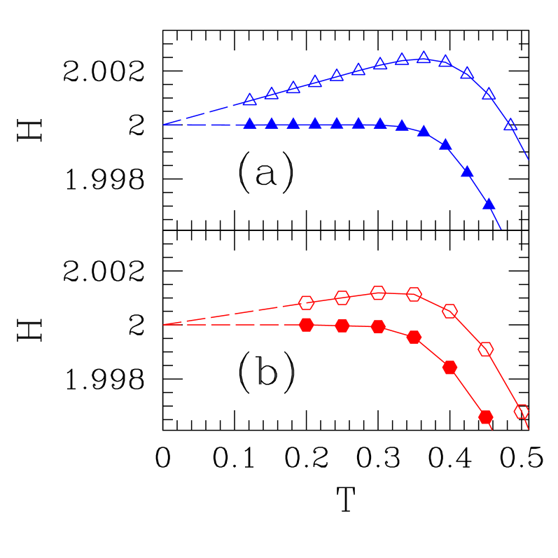
For $H\ll 1$, the solutions to Eq. (2) leave the $T$ axis vertically, and are very close to each other for all three orientations of the TM. We shall briefly return to this, towards the end of the paper. For low temperatures $T\lesssim 1$, the main region of interest here, substantial differences arise. These are illustrated in Fig. 1.

Figure 1: (Color online) Low-temperature approximate critical boundaries given by solutions of Eq. (2). Triangles, squares, and hexagons denote respectively TM along F, AF, and D direction. Empty symbols: $N=4$; full symbols: $N=22$ (F), $20$ (D and AF).

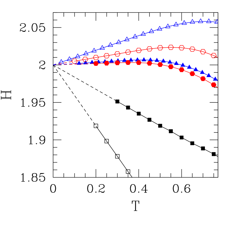
One sees that, with increasing $N$, all three families of curves get closer together, though AF does so at a slower rate. Also, in all cases their limiting shape for $T\lesssim 0.4$ is, with very good accuracy, a straight line going through the exact zero-temperature fixed point at $H=2$. Reentrant behavior is clearly visible for the F curves and, to a lesser extent, for the D ones, though in both cases the peaks turn flatter as $N$ increases. In order to check whether the reentrancies vanish in the $N\to\infty$ limit, we plotted the sequences of slopes $S_{N}$ of the $T\to 0$ straight-line sections referred to above, against $N^{-1}$.

Figure 2: (Color online) Slopes $S_{N}$ of the low-temperature straight-line sections of approximate critical boundaries given by solutions of Eq. (2), against $1/N$. Triangles, squares, and hexagons denote respectively TM along F, AF, and D direction. For AF, data are scaled by a factor of 5. Lines are fits to data: linear for F and D (all $N$), and parabolic (linear plus quadratic) for AF ($N\geq 10$ only).

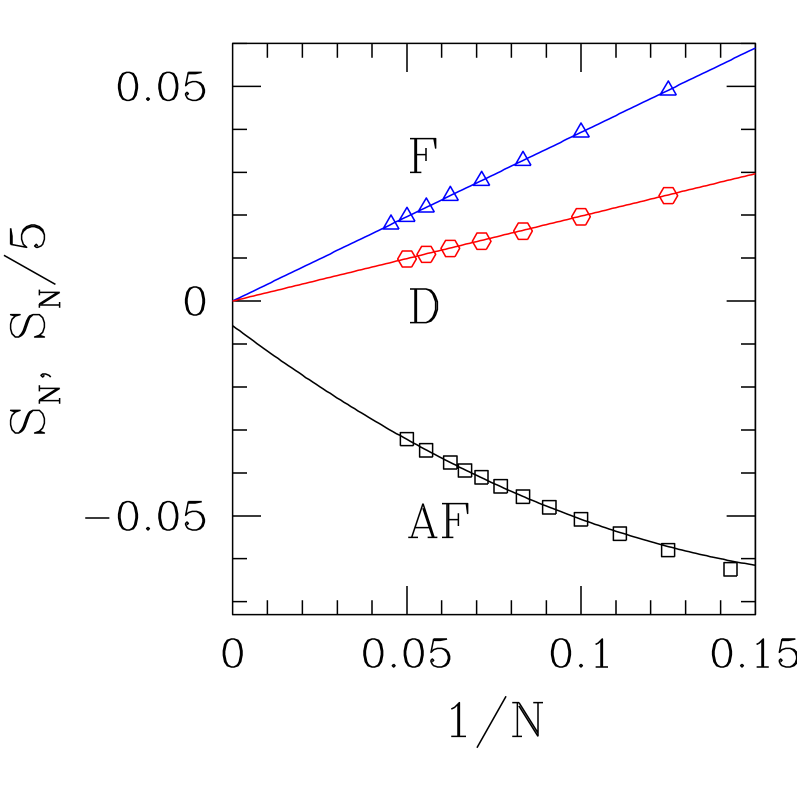
Results are shown in Fig. 2. For both F and D the trend is, to an excellent approximation, $S_{N}\to 0$ linearly with $N^{-1}$. Indeed, the respective extrapolated values are $(4\pm 3)\times 10^{-7}$ (F) and $(-15\pm 4)\times 10^{-5}$ (D), which in practice equate to zero within the present context. For AF, a large amount of curvature is present; from a parabolic fit ($S_{N}=S_{\infty}+a\,N^{-1}+b\,N^{-2}$) of $N\geq 10$ data, one gets $S_{\infty}=-0.029\pm 0.004$. This would correspond to $1-H_{c}(T)/H_{c}(0)\simeq 0.01$ at $T=0.5$ which, though small, is significant.

In summary, the analysis of limiting slopes at low $T$, $N\to\infty$, indicates that the reentrant behavior observed for F and D data is a finite-size effect, which tends to vanish in the thermodynamic limit. A small discrepancy still remains, between F and D data which are consistent with a horizontal critical line at $T\to 0$, and AF results which point to a slightly negative slope in that limit.

II.2 Phenomenological Renormalization

Further insight can be gained by relaxing the assumption made in Eq (2), that the phase transition belongs to the Ising universality class, and demanding only that it remain of second order. From finite-size scaling, one gets the basic equation of the phenomenological renormalization group (PRG) fs2 for the critical line:

$$N\kappa_{N}(T,H)=N^{\prime}\kappa_{N^{\prime}}(T,H),$$ (3)

where the strip widths $N$ and $N^{\prime}$ are to be taken as close as possible for improved convergence of results against increasing $N$. This means $N^{\prime}=N-2$ for F, D, and $N-1$ for AF.

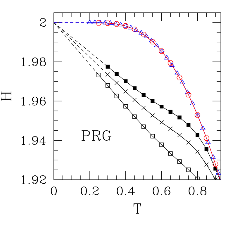
We found that PRG results converge very rapidly for both F and D orientations of the TM, without any sign of the reentrances shown by the solutions of Eq. (2). For the F case, the largest discrepancies between $N=6$ and $8$ amount to $0.8\%$ close to $H=0$, and are slowly reduced upon increasing $H$; around $T\simeq 0.7$, $H\simeq 1.97$, the two curves differ by $0.04\%$. At $T=0.4$, both coincide to within two parts in $10^{5}$, at less than $0.1\%$ of $H=2$, and then home in towards $(T,H)=(0,2)$ on a straight line. The discrepancy between $N=12$ and $14$ is never more than one part in $10^{4}$ for $T\leq 1$. The picture is quantitatively similar for the D orientation.

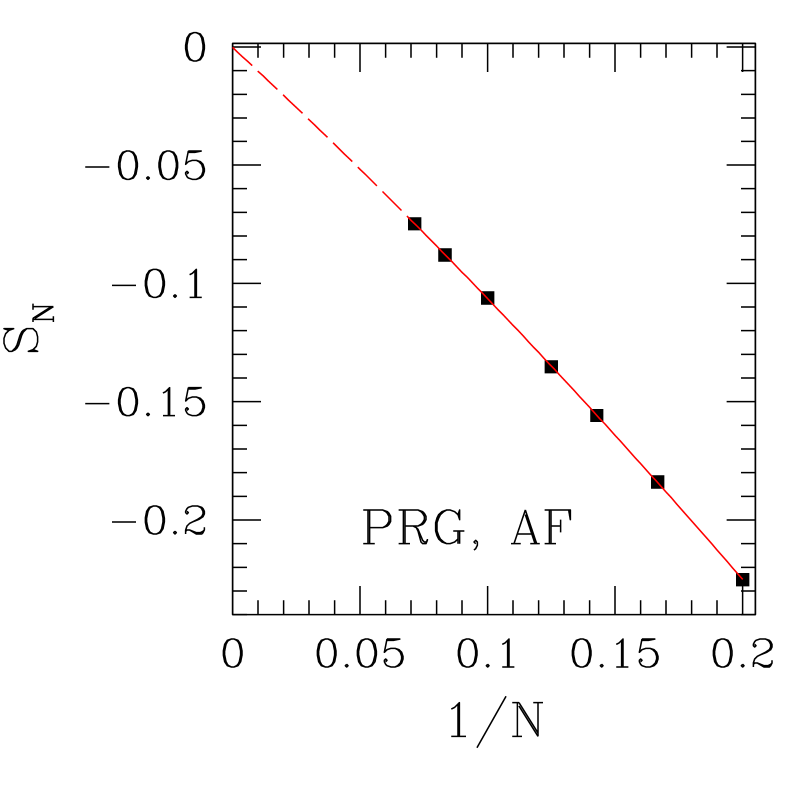
On the other hand, for PRG with the TM along the AF direction, one gets relatively large negative slopes (but approaching zero with increasing $N$) as $T\to 0$. Furthermore, at intermediate temperatures $0.4\lesssim T\lesssim 0.8$ the curves show inflection points which make extrapolation of such sections to $N\to\infty$ prone to instabilities.

Figure 3: (Color online) Low-temperature approximate critical boundaries given by solutions of Eq. (3). Triangles: TM along F direction, $N=14$; hexagons: D, $N=14$; empty squares, crosses, and full squares all for AF, respectively $N=10$, $12$, and $14$.

Figure 4: (Color online) Slopes $S_{N}$ of the low-temperature straight-line sections of approximate critical boundaries given by the solution of Eq. (3), for TM in the AF direction, against $1/N$. Data points are for $N=5-14$. The line is a parabolic (linear plus quadratic) fit to data.

The above-mentioned features are illustrated in Fig. 3. We investigated the behavior of the limiting slopes for the AF family against $1/N$, with results displayed in Fig. 4. The line shown in the Figure is a parabolic fit to data ($S_{N}=S_{\infty}+a\,N^{-1}+b\,N^{-2}$), from which one gets $|S_{\infty}|<10^{-3}$, i.e., essentially zero.

II.3 Extrapolations

In this Subsection, we deal directly with extrapolations of finite-size data for all $(T,H)$. This is in contrast to the analysis of slopes, which applies only at low $T$ where the finite-$N$ data actually fall on straight lines.

Extensive investigation of the related problem of isotropic Ising antiferromagnets in a field bdn88 shows that, in that case, the main irrelevant exponent is $y_{\rm ir}=-2$, i.e., the leading corrections to scaling are expected to depend on $N^{-2}$. Thus, it is plausible to assume that such corrections also play a dominant role here. However, the analysis of slopes above suggests that corrections in $N^{-1}$ are present as well, at least in the low-temperature region.

In what follows, we examine both scenarios, i.e., $y_{\rm ir}=-1$ and $-2$. The locations of points on the approximate critical line, for strip width $N$, are denoted by $(T_{N}^{\ast},H_{N}^{\ast})$. On account of the overall shape of the phase diagram, we extrapolate against negative powers of $N$ in two different ways: (i) at constant $X=H$ for high $T\gtrsim 1.7$, and (ii) at constant $X=T$ for $T\lesssim 1.7$. For large $N$, we fit $Y_{N}$ [$=T_{N}^{\ast}(H)$ in (i), or $H_{N}^{\ast}(T)$ in (ii)] to a form

$$Y_{N}^{\ast}(X)=Y_{\rm ext}(X)+a_{\,y_{\rm ir}}(X)\,N^{\,y_{\rm ir}}+b_{\,y_{\rm ir}}(X)\,N^{2y_{\rm ir}}\ .$$ (4)

We have chosen to calculate $Y_{\rm ext}(X)$, $a_{\,y_{\rm ir}}(X)$, and $b_{\,y_{\rm ir}}(X)$ from the three largest values of $N$ available for each strip orientation, thus error bars (other than those associated to the positions $Y_{N}^{\ast}(X)$ themselves) are not available from this procedure.

We managed to produce well-behaved extrapolated critical lines from the solutions to Eq. (2), only for F and D orientations of the TM. For AF, though extrapolations are generally smooth for $T\gtrsim 0.6$, they display instabilities for lower $T$, i.e. the section of the phase diagram which is most relevant in the search for reentrant behavior. As regards PRG curves, due to the fast convergence of F and D data we found that $N=14$ data can already be taken as very close to the $N\to\infty$ limit, to within an estimated one part in $10^{4}$. As mentioned above, the extrapolated PRG curves for AF display instabilities, except for very low $T$ (for which the relevant information is summarized in the slope analysis illustrated in Fig. 4).

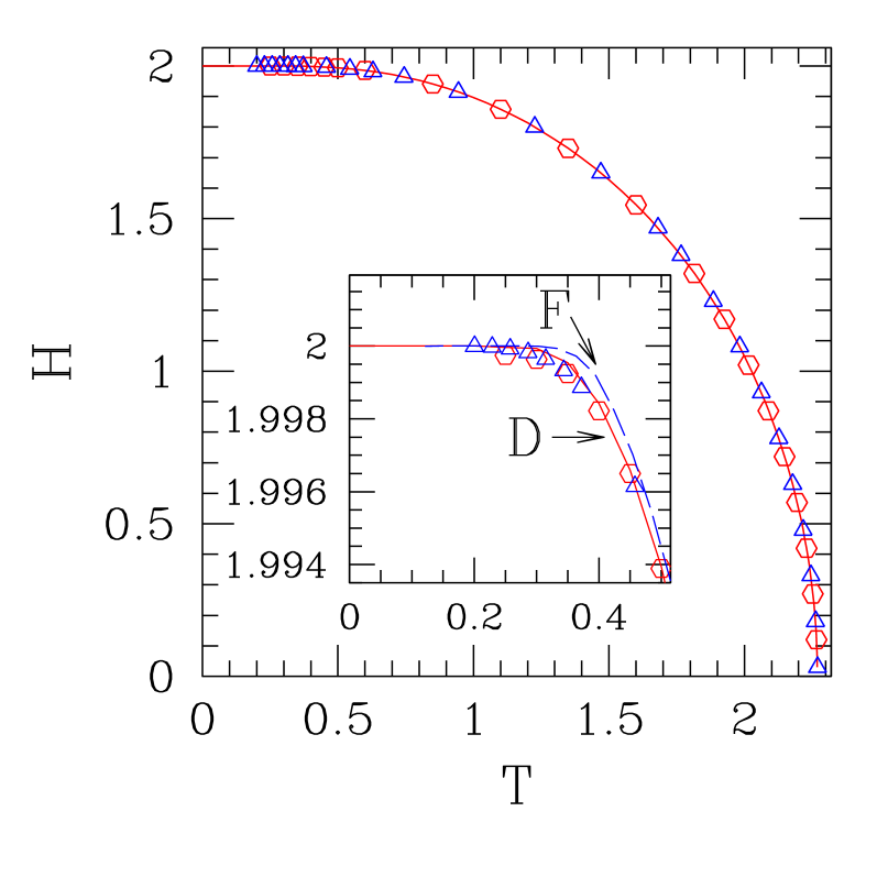
Fig. 5 shows the low-temperature regions of extrapolated critical boundaries, for F and D, assuming $y_{\rm ir}=-1$ or $-2$ in Eq. (4). For both curves corresponding to $y_{\rm ir}=-1$, there is a rather flat section: for F, points with $T\leq 0.36$ remain within one part in $10^{5}$ from $H=2$, while for D the $T\leq 0.35$ region is within one part in $10^{4}$ from that limit. On the other hand, the $y_{\rm ir}=-2$ extrapolations exhibit tiny reentrances, with maxima respectively at $H=2.0024$ (F) and $H=2.0012$ (D).

Figure 5: (Color online) Low-temperature extrapolated critical boundaries, obtained via Eq. (4), with $y_{\rm ir}=-2$ (empty symbols), and $y_{\rm ir}=-1$ (full symbols). TM is in the F direction in (a), and along the diagonal (D) in (b).

In order to get further insight into the competing scenarios under investigation, we examine the behavior of the coefficients $a_{-1}$ and $b_{-1}$ of Eq. (4) along the critical line. Indeed, this amounts to an unbiased test of whether the dominant $N$- dependence of finite-size data is on $N^{-1}$ (via $a_{-1}$) or $N^{-2}$ (via $b_{-1}$).

Figure 6: (Color online) Low-temperature behavior of fitting coefficients $a_{-1}$ (empty symbols), $b_{-1}$ (full symbols) of Eq. (4). Triangles: TM along F direction. Hexagons: TM along diagonal (D). Inset: high-temperature behavior. Same axis labels and symbol captions as in main figure (see text).

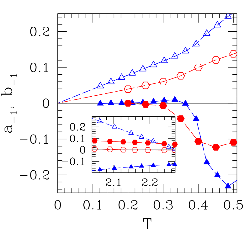
In Figure 6 one sees that, at low $T$, the $N^{-2}$ terms tend to vanish for both F and D cases. Furthermore, the inset of the Figure shows that in the low-field limit, it is the $N^{-2}$ corrections that become dominant, and those in $N^{-1}$ become negligible as $H\to 0$, as is well known for the zero-field Ising model bdn88 ; dQ00 . The latter result gives further credence to the procedure just described, and thus to the conclusions reached regarding the low–$T$ regime.

Finally, we found no clear evidence that an exponent $y_{\rm vac}=-4/3$, associated to vacancy excitations, might be present bdn88 . This is because (i) at the F and D data clearly depend predominantly on $N^{-1}$ at low $T$, as already shown in the slope analysis; and (ii) the slope data for AF do not exhibit any significant improvement in quality of fit when plotted against $N^{-4/3}$ (compared to the parabolic fits in $N^{-1}$ of Figs. 2 and 4).

III Discussion and conclusions

We begin by recalling that Eq. (3) depends on the existence of an underlying diverging correlation length, thus its non-trivial fixed points correspond to a second-order transition. We only failed to find such points for low temperatures, generally $T\lesssim 0.2$. This is due to the extremely slow convergence of numerical results, connected to the very large ratio between positive and negative exponentials which are the TM states’ Boltzmann weights in that region. If a tricritical point were present, separating first- and second-order sections of the critical curve, one would expect spurious effects such as the "hooking" found for the three-dimensional version of the current problem hs72 . On the contrary, as long as we can find low–$T$ solutions to Eq. (3) they behave in the expected manner, i.e. homing in towards the exact $T=0$ fixed point at $H=2$. Furthermore, the extrapolated $\eta=1/4$ curves agree very well with the solutions of Eq. (3) down to $T=0.2$, and still extend somewhat further down to $T\approx 0.1$ Since, by conformal invariance, $\eta=1/4$ corresponds to an Ising transition, our results indicate that this is the character of the critical line, at least down to $T=0.1$. Therefore, if a tricritical point is present, it must be located at $T<0.1$, $H\approx 2$. We thus conclude that the transition is indeed second-order and in the Ising universality class along the whole of the critical curve (except for the latter possibility, which we are not able to probe directly).

We now recall that the reentrant behavior predicted in Ref. wang97, is sizable: in the units used in the present work, it translates into the critical line leaving $(T,H)=(0,2)$ with a slope $S=(1/2)\ln 2=0.3466\dots$ [ see their Eq. (31) ]. This is in contrast with the results of Subsec. II.3, where we find at most $S=7\times 10^{-3}$ (with the TM in the F direction, using $y_{\rm ir}=-2$).

In the comparable problem of isotropic antiferromagnets, though the critical line $H_{c}(T)$ given in Ref. wang97b, does not exhibit reentrances, it is always above that found in Refs. ww90, ; bw90, (except at the $T=0$ and $H=0$ ends, where both lines coincide). The maximum discrepancy, of order $4\%$, is in the central region, $0.7\lesssim T\lesssim 1.5$, tailing off towards both ends. It thus appears that the methods employed in Refs. wang97b, ; wang97, generally tend to overestimate the extent of the ordered region in parameter space.

Though the present problem is weakly anisotropic in a broad sense, the distinct nature of spin couplings along each coordinate axis is responsible for the introduction of subtle biases, when one iterates the TM along either of those very same axes. Indeed, the size of the ordered region predicted by low-$T$ TM results systematically decreases as one changes orientation from F to D, and finally to AF. The explanation is that, for the high fields near the critical curve, the ferromagnetic correlations picked out when the TM goes along F tend to be emphasized; when the TM goes along AF, the corresponding antiferromagnetic correlations are inhibited by the field. The small negative extrapolated slope of the AF curves, shown in Fig. 2, most likely reflects the latter effect. For the TM going along D, an evenly-balanced mixture of both kinds of correlations is collected upon its iteration. Therefore we believe that, of the three setups implemented here, the latter is the one likely to produce the most reliable results.

Note also that, for PRG one is always comparing correlation lengths evaluated along the same lattice direction in Eq. (3), so the aforementioned biases tend to cancel out, if present. Thus, (i) the PRG curves for F and D do not show reentrancies, even for finite $N$; and (ii) the slope of PRG curves for AF approaches zero as $N^{-1}\to 0$ (see fig. 4), as opposed to the small negative value found for the corresponding solutions of Eq. (2).

In principle, the results for F, D, and AF orientations must eventually extrapolate to the same location of the critical boundary as $N\to\infty$. The way finite–$N$ data vary as $N$ increases is consistent with this, see Figs. 1 and 3. However, it is apparent that subdominant corrections to scaling have much larger amplitude for AF than for F or D. Attempting a theoretical understanding of why this is so usually becomes a highly nontrivial task, as it involves (i) unequivocally identifying the associated irrelevant exponents, and (ii) once this is done, analysing the (non-universal) amplitudes of the corresponding terms. Examples of this can be seen in Refs. bdn88, and dQ00, . Here, for practical reasons we chose to extrapolate only the sets of $(T,H)$ data for which the small subdominant corrections could be satisfactorily dealt with via Eq. (4) and its underlying assumptions.

We have found that the minimum amount of discrepancy among all our results corresponds to the set of: (i) extrapolated data from the solutions of Eq. (2), with the TM along D, using $y_{\rm ir}=-1$; (ii) PRG with the TM along D, and (iii) PRG with the TM along F. See Fig. 7. The extrapolations from the solutions of Eq. (2), with the TM along F, and using $y_{\rm ir}=-1$, also agree very well with these, except for the low-temperature ’shoulder’ where curves begin to depart more significantly from the horizontal line $H=2$. This is illustrated in the inset of Fig. 7.

Figure 7: (Color online) General view of extrapolated phase diagram. Full line is extrapolation of solutions of Eq. (2), with the TM along D, using $y_{\rm ir}=-1$. Points: PRG, $N=14$, with the TM along F (triangles) and D (hexagons). Inset: Low-temperature section of same data. Same axis labels and symbol captions as in main figure, except for additional dashed line which is extrapolation of solutions of Eq. (2), with the TM along F, using $y_{\rm ir}=-1$.

Figure 8: (Color online) Thermal scaling exponent $y_{T}=1/\nu$ along extrapolated critical line shown in Fig.7, calculated via Eq. (5), with $M=N-2$. TM along D. The discontinuity at $T\approx 1.74$ marks the change in assumed scaling direction (see text).

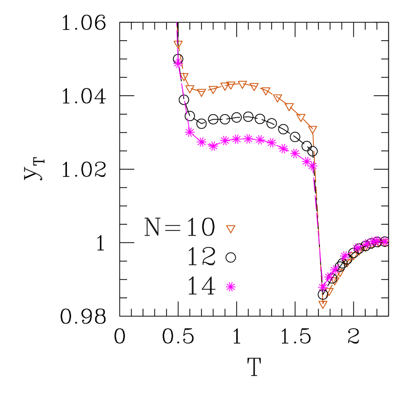
In order to check on the universality of critical properties, we examined the thermal exponent $y_{T}=1/\nu$ along the critical line. Considering two strips of widths $M$ and $N$, finite-size scaling fs2 gives:

$$y_{T}=1+\frac{\ln(\kappa_{N}^{\prime}/\kappa_{M}^{\prime})}{\ln(M/N)}\ ,$$ (5)

where $\kappa_{N}^{\prime}$, $\kappa_{M}^{\prime}$ are derivatives of the inverse correlation lengths, taken with respect to the appropriate temperature-like scaling field, evaluated on the critical curve. With the TM along D, and using $M=N-2$, we swept the extrapolated line shown in Fig. 7. For simplicity, the temperature-like direction was taken as the temperature axis for low and middle fields $H<1.41$ (corresponding to $1.74\lesssim T\leq 2.269\dots$), and as the $H$-axis for the remainder of the critical line. The resulting solutions to Eq. (5), for $N=10$, $12$, and $14$, are shown in Fig. 8. Although the abrupt jump at $T\approx 1.74$ is an artifact, reflecting the above-mentioned (and somewhat arbitrary) change in the assumed scaling direction, one sees that on both sides of the discontinuity the estimates are rather close to the Ising value $y_{T}=1$, and systematically approach it with increasing $N$. On the other hand, for $T\lesssim 0.5$ (where $H$ already differs by less than $0.5\%$ from the zero-temperature $H_{c}(0)=2$), crossover effects related to the energy level crossings at $T=0$ cause an extreme deterioration in our estimates.

Near the $H=0$ extreme of the critical curve, we have fitted our extrapolated curves to a parabolic shape:

$$T_{c}(H)=T_{c}(0)-a\,H^{2}\ ,$$ (6)

from which we get $a=0.217\pm 0.001$, to be compared with $a=0.1767\dots$ and $a=0.3018\dots$, each coming from a slightly different implementation of the interface method rottman90 . Note that the coefficient of a hypothetical linear term in Eq. (6) vanishes identically because the phase diagram is symmetric under field inversion, thus the scaling variable must depend on $H^{2}$. For $H\to 0$ this means that $T_{c}(H)=T_{c}(0)-aH^{2}$ plus higher-order terms mk87 .

Finally, we return to the exponentially vanishing deviations from a horizontal line near $T=0$, predicted in earlier work and mentioned in the Introduction. These are of the general form rottman90

$$H=2+c\,T^{x}\,\exp(-d/T)\ ,$$ (7)

where $c<0$ for both implementations of the interface method rottman90 , as well as for a free-fermion approximation rottman90 , whereas $c>0$ for the linear-chain approximation cg79 ; rottman90 ($|c|$, $d$, and $x$ turn out to be of order unity in all cases). While we do not have enough accuracy at low temperatures to probe for this sort of effect, it seems safe to state that any stronger deviations from the horizontal, be they in the shape of a reentrance or the opposite, are ruled out by our results.

Our extrapolated data for the location of the critical line, for both F and D, with $y_{\rm ir}=-1$ and $-2$, are available as ASCII files epaps .