A numerical investigation of the jamming transition in traffic flow on diluted planar networks

————————————————————————————————————

Abstract. In order to develop a toy model for car’s traffic in cities, in this paper we analyze, by means of numerical simulations, the transition among fluid regimes and a congested jammed phase of the flow of kinetically constrained hard spheres in planar random networks similar to urban roads .
In order to explore as timescales as possible, at a microscopic level we implement an event driven dynamics as the infinite time limit of a class of already existing model (Follow the Leader) on an Erdos-Renyi two dimensional graph, the crossroads being accounted by standard Kirchoff density conservations. We define a dynamical order parameter as the ratio among the moving spheres versus the total number and by varying two control parameters (density of the spheres and coordination number of the network) we study the phase transition.
At a mesoscopic level it respects an, again suitable adapted, version of the Lighthill-Whitham model, which belongs to the fluid-dynamical approach to the problem.
At a macroscopic level the model seems to display a continuous transition from a fluid phase to a jammed phase when varying the density of the spheres (the amount of cars in a city-like scenario) and a discontinuous jump when varying the connectivity of the underlying network.

————————————————————————————————————

1 Introduction

In the past decades an always increasing interest has been payed to the flow of cars in urban roads (see e.g. [1] or [2] for a beautiful modern review): a primary challenge is the reduction of time delays and CO emissions, in a nutshell, the congested traffic flow [3].
Despite progresses developed by engineers and physicist (see i.e. [4, 5]), essentially focused on large streets or small tree-like graphs [6, 7], very little is known concerning the behavior of traffic on large two dimensional networks [2].
In a completely different context, the last twenty years saw the statistical mechanics of disordered and complex systems [8] experience an increasing development as well as its range of applicability (see for instance [9, 10, 11]) and, inspired by these successes, we want to investigate the nature of the transition among a fluid state and a jammed counterpart in traffic flow on planar networks, investigating the presence (or the lacking) of criticality [12, 13] within a out of equilibrium statistical mechanics framework [14, 15].
Furthermore, statistical mechanics of disordered systems recently pointed out a deep connection among replica symmetry breaking scenario [16, 8], the paradigm of the transition among fluid and glass and the $P\rightarrow NP$ transition in problem solving of hard satisfiability problems [17, 18].
Interesting, if the mapping among jamming transition and $P\rightarrow NP$ completeness would apply to traffic jams too, it would vanish every attempt to an online control of car flow by external massive macro-computing giving more firm ground to interacting local optimizers (as i.e. neural networks) [19, 20, 21].
Deepening our knowledge concerning the jam transition in traffic flow should be then of great importance, in our traffic optimization planning, if, varying tunable parameters, glassy-like criticality arises [22].
From a practical viewpoint, as a rigorous formulation of out of equilibrium statistical mechanics is far from being exhausted [23, 24, 14], we do not have a paved mathematical way to follow for checking i.e. the involved time-scales [25] or the reach of a stationary state [26] (which is a primary requirement for giving meaning to the averages) and consequently there is the need of fastest simulation algorithms [27, 28] to cover as timescales as possible.
Even though we will move toward a molecular-dynamics-like approach [29], we stress that for similar reasons the biggest amount of works on this subject uses in fact cellular automata [30, 31, 5, 32] which are quite faster than the continuous models [33, 34, 35].
Fast simulations are in fact hard tasks, especially in models with continuum potentials as they need to be made discrete generally by using Trotter expansions of the Liouvillean [29] describing the motion in the phase space, forbidding a very long simulation time (i.e. by Liapounov constrictions [36]).
Avoiding these potentials, a very fast integration of the dynamics is offered by the Verlet event driven dynamics of hard spheres [37]: these spheres are without a real potential; they move on straight lines, up to a core distance at which they touch one-other and they feel an infinite barrier of potential which converts instantaneously the kinetic energy into potential energy.
In this way the motion against two successive collisions does not require integration. It is in fact propagated from collision to collision, the new positions and momenta are worked out by imposing conservation of particles (Kirchoff rule), energy and momenta, (we will preserve just the Kirchoff rule in our framework) and the motion is propagated again and so on [38] (we emphasize that this approach has been tackled also to granular systems [39], which are glassy systems sharing several features with traffic flow [40, 41]).
Of course there exist already several very sharp models for traffic flow but we introduce our one because we are moving in an opposite way for a different scope with respect the standard approach: as we want a large amount of cars as well as long simulation time for a thermodynamical approach, we allow ourself to skip as details of the motion as possible, retaining just the main features (as usually happens when looking at criticality in statistical mechanics [42]).
Once defined the microscopic dynamics we then focus at first at the mesoscopic level (order $10^{2}$ cars) to recover the Lighthill-Whitham scenario [43], for showing consistence with pre-existing works, then we focus on a macroscopic scale (up to $10^{4}$ cars) to study its thermodynamics. We introduce the ratio of the moving particle as a standard dynamical order parameter [2], labeled by $\phi$ that we call fluidity for the sake of clearness, and define it as

$$\phi=1-N^{-1}\sum_{i}^{N}v_{i},\ v_{i}\in[0,1]$$ (1.1)

(such that it is trivially one in the jammed phase (where there is no longer any motion) and decreases toward zero in the liquid phases) and study its behavior: average, distribution and fluctuations.
The model seems to display a jammed phase where the fluidity is strictly zero and its fluctuations are delta-like centered on the average (the congested phase where all the spheres are caged among their nearest neighbors) and a flowing phase in which the fluidity seems to decrease continuously to zero (cages smoothly disappear) by decreasing the density or discontinuously by increasing the connectivity and its fluctuations appear Gaussians.
The whole suggesting the model undergoes a second order like transition in the density and a first order like in the connectivity.
For the sake of clearness we aim to label with $\alpha$ the connectivity of the network, with $\rho$ the density of the $N$ cars (even thought, from practical comparison of different size networks it will be sometimes easier to deal directly with the un-normalized amount of car $N$) and with $v_{i}=v\ \forall i\in(1,...,N)$ the velocity of the $i^{th}$ car.
It is worth noting that the standard technique of statistical mechanics on diluted systems [44, 45] merges the two parameters via the relation $\alpha\tanh(\rho)=\rho^{\prime}$, $\rho^{\prime}$ being an equivalent density in a fully connected network, so actually do not display clearly the transition split among the two control parameters [46].
Furthermore we want to stress that there exist already works on dilute hard spheres in different contexts (as on the Bethe lattice) [47, 48] but, to our knowledge, not on networks with topology close to urban one.

2 Microscopic model

In this section we point out the simulation scheme, which, for the sake of simplicity we spit in two parts: the choice of the underlying network (the topology) and the choice of the dynamics on the network (the interactions).

2.1 The Network

At first we must introduce the graph. In order to mimic a real urban center we think at a graph whose links represent the roads and vertices represent intersections and end points. For their high connectivity, scale free [49] and fully connected [50] networks are inappropriate to describe such a graph and for the extremum order and homogeneity they present, also Voronoi tessellation [51] and regular grids are avoided [52].
Real data show a linear dependence among the number of roads versus the number of intersections [53], whose ratio must be obviously between one (tree like structures with no loops) and two ($2D$ regular lattice) with an empirical slope close to $3/2$ [54]. Even though clever growth algorithms for these networks recently developed [54], for computational simplicity (as we will have to average over several configurations and we want the fastest procedure) we choose the planar Erdos-Renyi graph [49] above the giant component threshold, which is close to the requested class of random graphs [55] and is of immediate realization on a computer as no growing is concerned.
All the links represent streets built by two lanes so to have both an incoming and an outgoing flux from each node.
On this network we can vary its averaged connectivity -the coordination number- (denoted by $\alpha$) so to explore from the region of extreme dilution near the percolation threshold up to a fully ordered grid.
Of course to check convergence to the infinite volume limit we will test our simulations varying also the size of the grid.

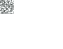
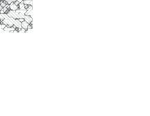
Figure 2.1: Examples of generated networks. At left an high connectivity topology, at right a low one. We start from a fully ordered grid in which each node has exactly $8$ links then we dilute the links with a Poisson distribution with mean $4$, such that the main nodes are ordinary crossroads. If a node has two, one or zero links is removed too.

2.2 The dynamics

On this network we let live $N$ cars for which we want to menage two limits at the same time (which conflict in terms of CPU time): the large $N$ limit to have enough data for the averages and the infinite time behavior so to approach to a steady state: the need of the fastest plausible algorithm follows straightforwardly.
One of the most important class of models which aim to mimic car dynamics is the so called follow the leader [56, 57, 6], where the dynamics of the $i^{th}$ car is assumed to respect the following differential equation (or some suitable variants [2]), where $(i+1)^{th}$ labels the car in front of the $i^{th}$, following the direction of motion:

$$\frac{d^{2}x_{i}}{dt^{2}}\sim(v_{i}-v_{i+1}).$$ (2.1)

In a nutshell the car $i$ accelerates if the car in front of is accelerating too (this happens both for positive and negative accelerations).
As a solution for the long time steady state behavior of the follow the leader model is given by the same constant velocity for all the cars (as it appears clearly by solving eq.(2.1) in the large time limit by imposing $d^{2}x_{i}/dt^{2}=0$) we choose for our microscopic dynamics an event driven hard-sphere-like dynamics [38], which is known to be one of the fastest achievable dynamics in terms of CPU time [28, 58] and is in agreement with these continuous potential in the regime where we are interested in ($t\rightarrow\infty$).
On every lane overtaking is forbidden (FIFO principle [57]) and every car has an energy $E_{i}=v^{2}_{i}/2$ during the free motion, whose dynamics is propagated between collisions among two cars or one car and a crossroad.
There the collision rules are worked out with a remarkable difference with respect to canonical physics: nor detailed balance neither the third law of dynamics do hold. When a collision happens there is no conservation of momenta and the incoming car loses all the energy then starts again following the collided car (crossroads apart which confer a certain degree of randomness), for this reason we call our hard spheres kinetically constrained [59, 60]. However as for instance elegantly explained in [61, 15] this is not a too serious limitation when investigating out of equilibrium steady state (the same is not true of course in equilibrium [42]).
The potential felt by the cars is the classical hard core potential [38, 28] $V$, which, by using $|x_{ij}|$ to evaluate the distance between the two cars situated respectively at $x_{i}$ and $x_{j}$, can be written as

$$V(|x_{ij}|)\equiv\left\{\begin{array}[]{rl}V_{0}=0\ \ \ \ \rm{if}\ \ \ \ |x_{ij}|\geq d\\ V_{1}=\infty\ \ \ \ \rm{if}\ \ \ \ |x_{ij}|<d\end{array}\right\}$$ (2.4)

where $d$ can be thought of as a security distance, the minimal distance allowed among two consecutive cars (we stress that varying $d$ changes also the maximum number of admitted cars inside a network $N_{max}$ -which sets $\rho=1$- and consequently the critical density for the transition, so we fix $d=1$ once for all).
So far we defined the network and the dynamics along a link (street); we must further specify what happens when more links merge in a node (crossroad): several decision rules can be implemented; in this preliminary work we impose a simple random walk at the nodes: if a car is at the end of a link and has $n$ possible directions to take it chooses one of them with probability $n^{-1}$.
Of course the total number of machines is conserved along the dynamics and we impose Kirchoff rules [2] for the flow at the nodes.

3 The adapted Lighthill-Whitham theory

As we want to move from a microscopic prescription toward a macroscopic description, there should be a mesoscopic lengthscale at which well known models, the most famous being the Lighthill-Whitham model (LW) [43], should be recovered. With mesoscopic we mean we are dealing with an ensemble of cars such that their concentration as a function of the space (labeled by $x$) and time (labeled by $t$) is meaningful whilst the average overall the concentrations can still be thought of in terms of a probabilistic description [62].
From a practical viewpoint let us now concentrate just on a big street with an amount $M$ of cars inside and analyze the flow at this level.
Assuming that the cars move from smaller to larger values of $x$, we define the concentration $C$ of an element of the traffic on the street as the amount of cars moving within the space delimited by two generic points $C\supset x\in[x_{a},x_{b}],\ x_{a}<x_{b}$. It follows that $C(x,t)=M^{-1}\sum_{i}^{M}(\theta(x_{i}(t)-x_{a})-\theta(x_{i}-x_{b}))$ and let us also write the velocity of the generic $i^{th}$ particle as $v_{i}(t)=1-\delta((x_{i}(t)+d)-x_{i+1}(t))$, such that if the car is moving, its velocity is one, otherwise is zero.
The traffic flow is defined as $J(x,t)=v_{g}(x,t)C(x,t)$ where $v_{g}(x,t)$ is the group velocity and $C(x,t)$ the concentration. Assuming conservation on the total amount of cars, the following continuity equation holds [43]

$$\frac{\partial C(x,t)}{\partial t}+\frac{\partial J(x,t)}{\partial x}=\sum_{i}^{N}\rho^{i}_{in}(x,t)-\sum_{j}^{N}\rho^{j}_{out}(x,t)$$ (3.1)

where $\rho^{i}_{in}(x,t)=\theta(x_{a}-x_{i}(t))-\theta(x_{a}-x_{b}-x_{i}(t))$ and $\rho^{i}_{out}(x,t)=1-\rho^{i}_{in}(x,t)$ take into account car entries and exits on the street.
The group velocity relates to the local velocity of the particles via [2] $v_{g}=\frac{1}{M}\sum_{i}^{M}v_{i}+\frac{1}{M}C\partial_{C}\sum_{i}^{M}v_{i}\leq 1$ which in our case reads off as

$$v_{g}=\langle v_{i}\rangle-\big{\langle}\frac{1}{N}\sum_{i}^{N}v_{i}\big{\rangle}=1-\phi,$$ (3.2)

where the brackets average out the Dirac deltas on some measure (note that $v_{g}\leq\langle v_{i}\rangle$).
The scenario is as follows: as far as the system is completely un-frustrated (low density liquid) the group velocity corresponds to the single velocity; increasing density of cars (or decreasing the connectivity of the network) frustration arises and lowers the group velocity up to a threshold where the jamming transition starts and $v_{g}$ goes to zero such that the only solution to eq. (3.1) is $C(x,t)=C\in[0,1]$.
For the sake of simplicity let us consider a very long piece of a street without entries or exits such that the LW model in our case obeys the following partial differential equation

$$\frac{\partial C(x,t)}{\partial t}+(1-\phi)\frac{\partial C(x,t)}{\partial x}=0,$$ (3.3)

whose solutions are Galilean characteristics with slope $1-\phi$ and can be expressed by generic functions $f(x\pm(1-\phi)t)$ (cinematic waves [63]). If we now focus on two adjacent elements, $C_{1}(x,t),C_{2}(x,t)$ and suppose that $C_{1}(x,t)$ is in front of $C_{2}(x,t)$ in the direction of motion, we see that as far as their corresponding fluidities are zero they both follow straight lines (on the $x,t$ plane) with the same slope. If we now suppose that $C_{1}$ changes its status (for example by internal rearrangements, that we impose in the simulation by freezing randomly spheres belonging to the first package) and becomes frustrated $\phi_{1}>0$, its group velocity decreases and at the time $\Delta X/(v_{g1}(\phi)-v_{g2})$ the two characteristics meet causing a discontinuity in the concentration functions, which acts as the starter of the transition, as (due to the structure of the solution) it propagates both forward and backward on the street.

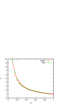
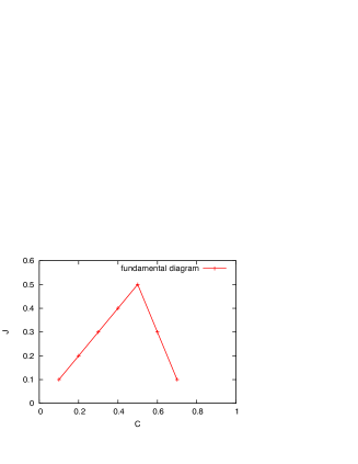
Figure 3.1: Left: Collision time versus the fluidity of the first concentration $C_{1}$ in our LW model, theor stands for analytical prediction, exp for the simulation results. Right: Fundamental diagram for our LW model.

4 Macroscopic behavior

Now we turn to the analysis on large scale networks. We consider three sizes of (squared) networks, which, at the highest connectivity, are completely filled by $N_{max}=2\times 10^{3}$, $5\times 10^{3}$ and $1\times 10^{4}$ spheres, which set $\rho=1$ in the different cities.
The connectivity ranges from $0$ to $1$ and is changed from the percolation threshold (which is defined by $\alpha=0$) to the fully two dimensional network (which is defined by $\alpha=1$) in eight steps and the density (again defined in $[0,1]$) is investigated at five different values too.
The analysis works as follows: for every investigated size, degree of connectivity and density, we average over twenty different runs; for every run we start off spheres randomly over the network (avoiding pathological overlaps) and study the mean of the fluidity, its variance and its distribution by starting to collect data when the mean does not vary sensibly (less than $5\%$ for an amount of time $O(10^{5})$ collisions), that we claim to be a stationary state.

At first, even though we do not provide a plot (as it would have just three points), we stress that we obtained good agreement among the three different city sizes investigating the monotonicity of the convergence of the averages (of fluidity and its variances), which is the basis of the thermodynamic limit (fundamental property for a well behaved model [64]).
For all the not-jammed stationary states (at fixed $\alpha,\rho)$ we analyzed the distribution of the fluidity sampling over the whole simulations performed: they turn out to be close to Gaussians distributions (which we use as a test fit, see figure (4.1)), the variance being almost independent by $\alpha$ and increasing with the density of the spheres up to the transition point (at given $\alpha$), immediately later they are delta-like on the averaged of the fluidity ($\phi=1$).

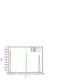
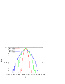
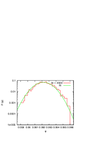
Figure 4.1: Fluidity fluctuations in the steady state for the largest size city at a connectivity $\alpha=0.6$: We show the distributions of $3$ different densities ($N=1\cdot 10^{3},2\cdot 10^{3},3\cdot 10^{3}$) on a lin-lin scale (left), the spread of their variances, centering the distributions on the smallest average for easier visualization (center) and a Gaussian fit $(\chi^{2}\sim 0.93)$ on a log-scale obtained by sampling over $2000$ cars.

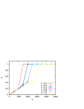
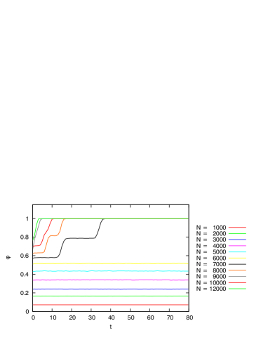
Figure 4.2: Left: Behavior of the fluidity versus the total number of cars at six different values of the connectivity. In the low density regime the dependence of $\phi$ versus $N$ is linear and universal. Right: Example of fluidity versus time on a single network (time is measured by the number of collisions (modulus $10^{4}$) showed from the larger city: there exist only two ”macroscopic” long term behavior: a jammed phase, that for the investigated values appears for $N\geq 7\times 10^{3}$ and a liquid phase, which however shows a continuous variation in the fluidity versus the density of cars (for $N<7\times 10^{3}$).

The average fluidity versus the density (that we plot directly by using the amount of cars) is shown in figure (4.2): For low density regimes, flow behavior appears independent by the connectivity of the network (and the scaling is always the same $\phi\propto\rho$), while, for higher values of the density a second regime is approached which is highly sensible by the connectivity, and in which, continuity of the order parameter with respect to the density is still observed.
Finally, for highest level of density a discontinuous jump to the jammed phase is observed, for all the values of the connectivity (see figure (4.3) where we report results for the medium city size).

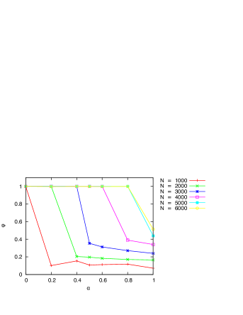
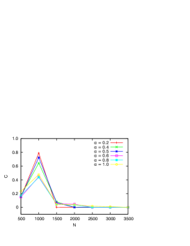
Figure 4.3: Left: Medium city. Behavior of the fluidity versus the connectivity for five different densities, shown in terms of the total amount of cars $N$. Right: Smallest city. self-averaging $C$ of the order parameter: fluctuations versus the density (expressed in terms of the total amount of cars), for six different connectivity values. The onset of the jam transition is shown by the peak, which, increases proportionally to $\alpha^{-1}$.

In figure (4.3) furthermore we show the fluctuations of the order parameter for the smallest city: it is worth noting that a phase transition (marked by a sharp peak inversely proportional to the connectivity) seems to appear at a critical value of density. Analyzing again the medium size city, we show in figure (4.3) the behavior of the order parameter versus the connectivity (for several values of density) and there is no presence of a continuous behavior: at a critical value (depending on the density) a jump to a jammed phase is observed.

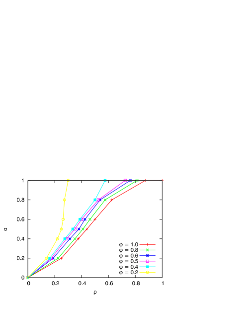
Figure 4.4: Phase diagram: The line $\phi=1$ is the transition line. At right there is the jammed phase at left the fluid phase. Further, the latter is shown split in six zones accordingly with different values of the fluidity.

5 Conclusions

In this paper we implemented a numerical algorithm which mimics the flow of cars in urban cities: cars are described as kinetically constrained hard spheres and urban topology is chosen as a planar Erdos Renyi graph. Kinetically constrained because the one way roads break detailed balance and the collisions among two cars do not respect the third law of thermodynamics. Even though mathematically hard to be analyzed, this model can still be investigated by numerical simulations. Hard spheres because, as in principle we do not know how many timescales are involved in the genesis of the congested phase, and being interest in the long time behavior, we have chosen one of the fastest possible algorithms for the dynamics: the event driven motion, which requires hard spheres. We investigated the response of a dynamical order parameter, the fluidity, defined as the ratio among the moving cars on the whole ensemble, by tuning two control parameters: the density of the cars and the connectivity of the network.
From this numerical investigation we found a continuous transition from a congested phase to a fluid phase by varying the density of the cars (at fixed connectivity) such that the fluidity lowers smoothly from $1$ to smaller values (up to zero where there are no longer cars) and a discontinuous jump of this order parameter when varying the connectivity of the network at fixed amount of cars.
Furthermore the timescales involved seem to be several (the longest of which seems to diverge at the transition to a jammed phase) rising the question on what kind of traffic optimizer should be developed in order to minimize traffic.
On these first heuristic considerations we believe that interacting local optimizers (as a grid of interacting cross-lights able to detect flow [57, 65]) would work better than a global ground state searcher and are more stable with respect to perturbations as new added (or removed) streets.
Future works concerning the kind of transition will be due to investigate the relaxation to equilibrium after the stimuli by introducing a car (or a few) or by introducing a new link, so to check the presence of aging in the network. Furthermore traffic optimization by properly interacting traffic lights will be considered as well.

References

- [1] A.D. May, Traffic Flow Fundamentals, Prentice-Hall (1990).
- [2] D. Chowdhury, L. Santen, A. Schadschneider, Statistical Physics of Vehicular Traffic and some related systems, Phys. Rep. 199, (2000).
- [3] The urban mobility report, Texas Transportation Institute, (2005).
- [4] D. Helbing, Traffic and related self-driven many-particle systems, Rev. Mod. Phys. 73, (2001).
- [5] K. Nagel, J. Esser and M. Rickert, in: Annu. Rev. Comp. Phys., ed. D. Stauffer, World Scientific (1999).
- [6] M. Bando, K. Hasebe, A. Nakayama , A. Shibata, Y. Sugiyama, Dynamical model of traffic congestion and numerical simulation, Phys. Rev. E 51, 1035 - 1042 (1995).
- [7] T. Nagatani, Chaotic jam and phase transition in traffic flow with passing, Phys. Rev. E 60, no. 2 1535 1541 (2001).
- [8] M. Mézard, G. Parisi and M. A. Virasoro, Spin glass theory and beyond, World Scientific, Singapore (1987).
- [9] F. Guerra, An introduction to mean field spin glass theory: methods and results, In: Mathematical Statistical Physics, A. Bovier et al. eds, , Elsevier, Oxford, Amsterdam, (2006).
- [10] A. Engel, C. Van den Broeck, Statistical Mechanics of Learning Cambridge University Press (2001).
- [11] D.J. Amit, Modeling brain function: The world of attractor neural network Cambridge Univerisity Press, (1992)
- [12] H.E. Stanley, Introduction to Phase Transitions and Critical Phenomena, Oxford University Press, (1971).
- [13] A. Barra, L. De Sanctis, V. Folli, Critical behavior of mean-field spin glasses on a dilute random graph, J. Phys. A: Math. Theor. 41 No 21 (2008) 215005
- [14] D.J. Evans and G.P. Morris, Statistical Mechanics of Non-Equilibrium Liquids, Academic, London, (1990);
- [15] G. Ciccotti and G. Kalibaeva, Molecular dynamics of complex systems: non-Hamiltonian, constrained, quantum-classical, ”Novel methods in soft matter simulation” Karttunen, Vattulainen and Lukkarinen Edr., Springer Verlag (2004).
- [16] A. Barra, L. De Sanctis, On the mean field spin glass transition, Europ. Phys. Jour. B - Condensed Matter and Complex Systems 64, 1, 2008
- [17] M. Mezard, G. Parisi, R. Zecchina, Science 297, 812, (2002).
- [18] L. Correale, M. Leone, A. Pagnani, M. Weigt, R. Zecchina, Core percolation and onset of complexity in Boolean networks, Phys. Rev. Lett. 96, 018101 (2006).
- [19] V. Honavar, L. Uhr (Ed.) Artificial Intelligence and Neural Networks: Steps Toward Principled Integration, Elsevier, Boston: Academic Press (1994).
- [20] A.C.C. Coolen, R. Kuehn, P. Sollich, Theory of Neural Information Processing Systems Oxford University Press, (2005)
- [21] A. Barra, F. Guerra, The ergodic region of the analogical Hopfiel neural network, to appear in J. Math. Phys. (2008).
- [22] L. F. Cugliandolo, J. Kurchan, L. Peliti, Energy flow, partial equilibration, and effective temperature in systems with slow dynamics. Phys. Rev. E 55, 3898, (1997).
- [23] G. Gallavotti, E.G.D. Cohen, Phys. Rev. Lett. 74, 2694-2697 (1995); J. Stat. Phys. 80, 931-970 (1995).
- [24] K. Kawasaki, Correlation-Function Approach to the Transport Coefficients near the Critical Point, I . Phys. Rev. 150, 291 (1966).
- [25] J. van Mourik, A.C.C. Coolen, Cluster Derivation of Parisi’s RSB Solution for Disordered Spin Systems, J. Phys. A 34, L111-L117 (2001).
- [26] Bridging time scales: Molecular simulations for the next decade, SIMU Conference, Konstanz (2001), P.Nielaba, M.Mareschal, and G.Ciccotti, Eds., Springer, Berlin, (2003).
- [27] Computer Simulations in Condensed Matter: From Materials to Chemical Biology, M.Ferrario, G.Ciccotti, and K.Binder Eds, LNP, Springer Verlag, Berlin, (2006).
-
[28]
A. Barra, M. Di Pierro, G. Kalibaeva, Algorithms for the dynamics of bond-constrained hard sphere
polymers,
preprint http://abaddon.phys.uniroma1.it/uploads/Main/BdPK.pdf (2007) - [29] D. Frenkel, B. Smith, Understanding Molecular Simulation: From Algorithms to Applications, Academic Press, (2002).
- [30] J. Esser and M. Schreckenberg, Microscopic simulation of urban traffic based on cellular automata, Int. J. Mod. Phys. B 8, no. 5 1025 1036, (1997).
- [31] S. Wolfram, Theory and Applications of Cellular Automata, World Scientific (1986); Cellular Automata and Complexity, Addison-Wesley, (1994).
- [32] K. Nagel and M. Schreckenberg, A cellular automaton model for freeway traffic, J. Phys. 2 , no. 12 2221 2229 (1992).
- [33] R. Herman and K. Gardels, Sci. Am. 209(6), 35 (1963).
- [34] D.C. Gazis, Science 157, 273 (1967).
- [35] R.W. Rothery, in: N. Gartner, C.J. Messner, A.J. Rathi (eds.), Transportation Research Board (TRB) Special Report 165, Traffic Flow Theory, 2nd ed. (1998).
- [36] C. Beck, F. Schogl, Thermodynamics of Chaotic Systems: An Introduction, Cambridge Nonlinear Science Series (2000).
- [37] Dennis C Rapaport, The Art of Molecular Dynamics Simulation, Cambridge University Press, (2004).
- [38] G. Ciccotti and G. Kalibaeva, Simulation of diatomic liquids using hard spheres model, J. Stat. Phys. 115, (2004).
- [39] G. Constantini, U. Marini Bettolo, G. Kalibaeva, G. Ciccotti, The inelastic hard dimer gas: a non-spherical model for granular matter, J. Stat. Phys. 132 (2005)
- [40] D.E. Wolf, M. Schreckenberg and A. Bachem (eds.), Traffic and Granular Flow, World Scientific, Singapore (1996).
- [41] M. Schreckenberg and D.E. Wolf (eds.), Traffic and Granular Flow, Springer, Singapore (1998).
- [42] K. Huang, Statistical Mechanics (2nd edition), John Wiley Pub., (1987).
- [43] M. Lighthill and G. Whitham, On Kinematic Waves: II. A Theory of Traffic Flow on Long Crowded Roads, Proc. Roy. Soc. Lond. Math. Phys. Sci. 229 (1955), no. 1178 317 345.
- [44] E. Agliari, A. Barra, F. Camboni, Criticality in diluted ferromagnet, J. Stat. Mech. 173308 (2008).
- [45] F. Guerra, F. L. Toninelli, The high temperature region of the Viana-Bray diluted spin glass model, J. Stat. Phys. 115 (2004).
- [46] Strictly speaking the investigated systems we meant are spins on lattice, whose order parameter is the temperature, which is well known, for model with discontinuous potentials, substituted by the density.
- [47] G. Biroli, M. Mézard, Phys. Rev. Lett. 88, 025501, (2001).
- [48] O. Rivoire, G. Biroli, O. Martin, M. Mézard, Eur. Phys. J. B 37, 55 (2004).
- [49] G. Caldarelli, Scale-free networks, Oxford Univ. Press (2008).
- [50] K. H. Fischer, J. A. Hertz, em Spin Glasses, Cambridge University Press, (1991).
- [51] A. Okabe, B. Boots, K. Sugihara, S. N. Chiu, Spatial Tessellations - Concepts and Applications of Voronoi Diagrams. John Wiley, (2000)
- [52] N. Ashcroft, N. Mermin Solid state physics, Camrbidge University Press, (1976)
- [53] A. Cardillo, S. Scellato, V. Latora, S. Porta, Phys. Rev. E 73 (2006).
- [54] M. Barthelemy, A. Flammini, Modeling urban street patterns, arXiv:0708.4360v2 (2008).
- [55] S. Gerke, C. McDiarmid, Random planar grap hs with nodes and fixed number of edges, Combinatorics, probability and Computing, 13 (2004).
- [56] I. Gasser, G. Sirito, B. Werner, Bifurcation analysis of a class of car following traffic models, Physica D: Nonlinear Phenomena Volume 197, Issues 3-4, 15 October (2004).
- [57] S. L mmer D. Helbink, Self-control of traffic lights and vehicle flows in urban road networks J. Stat. Mech. P04019 (2008).
- [58] Y. Weinbach, R. Elber, em Revisiting and Parallelizing SHAKE, Journ. Comp. Phys., 209:193-206 (2005).
- [59] Proceedings of workshop on Glassy dynamics in kinetically constrained models. Journal of Physics: Condensed Matter, 14 (7), P. Sollich, F. Ritort eds. (2002).
- [60] P. Sollich, F. Ritort, Glassy dynamics of kinetically constrained models, Advances in Physics, 52:219-342, (2003)
- [61] B. Derrida and M.R. Evans, in: Nonequilibrium Statistical Mechanics in One Dimension, Cambridge University Press, (1997), B. Derrida, Phys. Rep. 301, 65 (1998).
- [62] P. Sollich, A rheological constitutive equation for soft glassy systems, Phys. Rev. E 43, (1996).
- [63] G.B. Whitham, Linear and Nonlinear Waves, Wiley (1974); Lectures on Wave Propagation, Springer (1979).
- [64] F. Guerra, F. L. Toninelli, The Thermodynamic Limit in Mean Field Spin Glass Models, Commun. Math. Phys. 230:1, 71-79 (2002).
- [65] K. Sekiyama, J. Nakanishi, I. Takagawa, T. Higashi, and T. Fukuda, Self-organizing control of urban traffic signal network, IEEE Int. Conf. Syst. Man. Cybern. 4, 2481 2486 (2001).