Dark matter in minimal supergravity with type-II seesaw
Abstract
We calculate the relic density of the lightest neutralino in a supersymmetric seesaw type-II (“triplet seesaw”) model with minimal supergravity boundary conditions at the GUT scale. The presence of a triplet below the GUT scale, required to explain measured neutrino data in this setup, leads to a characteristic deformation of the sparticle spectrum with respect to the pure mSugra expectations, affecting the calculated relic dark matter (DM) density. We discuss how the DM allowed regions in the () plane change as a function of the (type-II) seesaw scale. We also compare the constraints imposed on the models parameter space form upper limits on lepton flavour violating (LFV) decays to those imposed by DM. Finally, we briefly comment on uncertainties in the calculation of the relic neutralino density due to uncertainties in the measured top and bottom masses.
I Introduction
Standard cosmology requires the existence of a non-baryonic dark matter (DM) contribution to the total energy budget of the universe Jungman:1995df ; Bertone:2004pz . In the past few years estimates of the DM abundance have become increasingly precise. Indeed, the Particle Data Group now quotes at 1 c.l. PDG2008
| (1) |
Since the data from the WMAP satellite Spergel:2003cb ; Komatsu:2008hk and large scale structure formation Tegmark:2006az is best fitted if the DM is cold, weakly interacting mass particles (WIMP) are currently the preferred explanation. While there is certainly no shortage of WIMP candidates (lists can be found in many reviews, see for example Jungman:1995df ; Bertone:2004pz ; Bergstrom:2009ib ; Baer:2009bu ), the literature is completely dominated by studies of the lightest neutralino.
Neutrino oscillation experiments have shown that neutrinos have non-zero mass and mixing angles Fukuda:1998mi ; Ahmad:2002jz ; Eguchi:2002dm ; Collaboration:2007zza ; KamLAND2007 and the most recent global fits to all data Maltoni:2004ei confirm again that the mixing angles are surprisingly close to the so-called tri-bimaximal mixing (TBM) values Harrison:2002er . In the minimal supersymmetric extension of the standard model (MSSM) with conserved R-parity neutrino masses are zero for the same reasons as in the SM. However, it was shown long ago that if neutrinos are Majorana particles, their mass is described by a unique dimension-5 operator Weinberg:1979sa
| (2) |
All (Majorana) neutrino mass models reduce to this operator at low energies. If is a coefficient , current neutrino data indicates GeV. This is the essence of the “seesaw” mechanism. There are three different tree-level realizations of the seesaw, classified as type-I, type-II and type-III in Ma:1998dn . Type-I is the well-known case of the exchange of a heavy fermionic singlet Minkowski:1977sc ; seesaw ; MohSen . Type-II corresponds to the exchange of a scalar triplet Schechter:1980gr ; Cheng:1980qt . One could also add one (or more) fermionic triplets to the field content of the SM Foot:1988aq . This is called seesaw type-III in Ma:1998dn .
Neutrino experiments at low energies measure only , thus observables outside the neutrino sector will ultimately be needed to learn about the origin of eq. (2). Augmenting the SM with a high-scale seesaw mechanism does not lead to any conceivable phenomenology apart from neutrino masses, but if weak scale supersymmetry exists indirect probes into the high energy world might be possible. Two kind of measurements containing such indirect information exist in principle, lepton flavour violating (LFV) observables and sparticle masses.
Assuming complete flavour blindness in the soft supersymmetry breaking parameters at some large scale, the neutrino Yukawa matrices will, in general, lead to non-zero flavour violating entries in the slepton mass matrices, if the seesaw scale is lower than the scale at which SUSY is broken. This was first pointed out in Borzumati:1986qx . The resulting LFV processes have been studied in many publications, for low-energy observables such as and conversion in seesaw type-I see for example Hisano:1995nq ; Hisano:1995cp ; Ellis:2002fe ; Deppisch:2002vz ; Arganda:2005ji ; Antusch:2006vw ; Arganda:2007jw , for seesaw type-II Rossi:2002zb ; Hirsch:2008gh . LFV collider observables have also been studied in a number of papers, see for example Hirsch:2008gh ; Hisano:1998wn ; Krasnikov:1995qq ; ArkaniHamed:1996au ; Nomura:2000zb ; Porod:2002zy ; Deppisch:2003wt ; delAguila:2008iz ; Deppisch:2005rv ; Bartl:2005yy ; Hirsch:2008dy ; Carquin:2008gv ; Esteves:2009vg .
Mass measurements in the sparticle sector will not only be necessary to learn about the mechanism of SUSY breaking in general, but might also reveal indications about the scale of the seesaw mechanism. However, very precise knowledge of masses will be necessary before one can learn about the high scale parameters Blair:2002pg ; Freitas:2005et . Especially interesting in this context is the observation that from the different soft scalar and gaugino masses one can define certain combinations (“invariants”) which are nearly constant over large parts of mSugra space. Adding a seesaw mechanism of type-II or type-III these invariants change in a characteristic way as a function of the seesaw scale and are thus especially suited to extract information about the high energy parameters Buckley:2006nv . Note, however, that the “invariants” are constants in mSugra space only in leading order and that quantitatively important 2-loop corrections exist Hirsch:2008gh .
In this paper we study neutralino dark matter Ellis:1983ew ; Griest:1990kh ; Drees:1992am within a supersymmetric type-II seesaw model with mSugra boundary conditions. For definiteness, the model we consider consists of the MSSM particle spectrum to which we add a single pair of - and -plets. This is the simplest supersymmetric type-II setup, which allows one to maintain gauge coupling unification Rossi:2002zb and explain measured neutrino oscillation data.
In mSugra - assuming a standard thermal history of the early universe 111In models with non-standard thermal history the relation between sparticle masses and relic density can be lost completely Gelmini:2006pw . - only four very specific regions in parameter space can correctly explain the most recent WMAP data Komatsu:2008hk . These are (i) the bulk region; (ii) the co-annihilation line; (iii) the “focus point” line and (iv) the “higgs funnel” region. In the bulk region there are no specific relations among the sparticle masses. However, all sparticles are rather light in this region, so it is already very constrained from the view point of low-energy data Allanach:2004xn . In the co-annihilation line the lightest scalar tau is nearly degenerate with the lightest neutralino, thus reducing the neutralino relic density with respect to naive expectations Griest:1990kh ; Baer:2002fv . In the “focus point” line Feng:1999zg ; Baer:2002fv is small enough to explain due to a rather small value of leading to an enhanced higgsino component in the lightest neutralino and thus an enhanced coupling to the boson. Lastly, at large an s-channel resonance pair annihilation of neutralinos through the CP-odd higgs boson can become important. This is called the “higgs funnel” region Drees:1992am .
The addition of the and pair at the high scale does not, in general, lead to the appearance of new allowed regions. However, the deformed sparticle spectrum with respect to mSugra expectations leads to characteristic changes in the allowed regions as a function of the unknown seesaw scale. We discuss these changes in detail and compare the results to other indirect constraints, namely, the observed neutrino masses and upper limits on LFV processes. We concentrate on the seesaw type-II scheme, since for mSugra + seesaw type-I the changes in the DM allowed regions with respect to pure mSugra are, in general, expected to be tiny. 222We have confirmed this general expectation with some sample calculations. However, an exceptional case has been presented recently in Kadota:2009vq , see the more detailed discussion in section (III).
The rest of this paper is organized as follows. In the next section we briefly summarize the main ingredients of the model and give a short discussion of mSugra and the expected changes in sparticle masses in our setup with respect to mSugra. In section (III) we present our numerical results. This is the main section of the current paper, where we discuss in detail how the introduction of a changes the predicted DM abundance as a function of the seesaw scale. We also confront the DM allowed regions with constraints from non-observation of LFV processes and briefly comment on DM in mSugra with a seesaw type-I. We then close with a short summarizing discussion in section (IV).
II Setup: mSugra and motivated type-II seesaw
In this section we summarize the main features of the model we will use in the numerical calculation. We will always refer to minimal Supergravity (mSugra) as the “standard” against which we compare all our results. The model consists in extending the MSSM particle spectrum by a pair of and . It is the minimal supersymmetric seesaw type-II model which maintains gauge coupling unification Rossi:2002zb .
mSugra is specified by 4 continuous and one discrete parameter Nilles:1983ge . These are usually chosen to be , the common scalar mass, , the gaugino mass parameter, , the common trilinear parameter, and the sign of . , and are defined at the GUT scale, the RGEs are known at the 2-loop level Martin:1993zk .
Under the decomposes as
| (3) | |||||
The invariant superpotential reads as
Here, , , and . Below the GUT scale in the -broken phase the potential contains the terms
, and generate quark and charged lepton masses in the usual manner. In addition there are the matrices , and . For the case of a complete , apart from calculable threshold corrections, and , and are determined from by the RGEs. As long as gauge coupling unification will be maintained. The equality need not be exact for successful unification.
The triplet has the correct quantum numbers to generate neutrino masses via the first term in eq. (II). Integrating out the heavy triplets at their mass scale a dimension-5 operator of the form eq. (2) is generated and after electro-weak symmetry breaking the resulting neutrino mass matrix can be written as
| (6) |
Here is the vacuum expectation value of Higgs doublet and we use the convention . can be diagonalized in the standard way with a unitary matrix , containing in general 3 angles and 3 phases. Note that is diagonalized by the same matrix as . This means that if all neutrino eigenvalues, angles and phases were known, would be completely fixed up to an overall constant, which can be written as . Thus, current neutrino data requires to be lower than the GUT scale by (at least) an order or magnitude.
The full set of RGEs for the + can be found in Rossi:2002zb and in the numerical calculation, presented in the next section, we solve the exact RGEs. However, for a qualitative understanding of the results, the following approximative solutions are quite helpful.
For the gaugino masses one finds in leading order
| (7) |
Eq. (7) implies that the ratio , which is measured at low-energies, has the usual mSugra value, but the relationship to is changed. Neglecting the Yukawa couplings (see below), for the soft mass parameters of the first two generations one gets
| (8) | |||||
| (9) |
The various coefficients can be found in Hirsch:2008gh . The gauge couplings are given as
| (10) | |||||
with and being the usual standard model and MSSM coefficients. for all in case of a complete 15-plet.
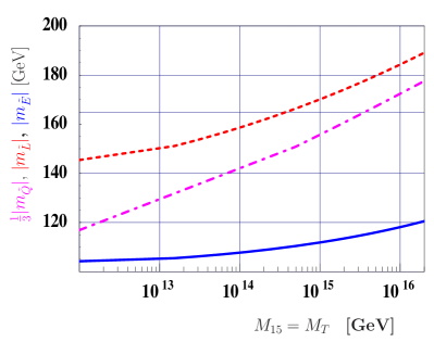
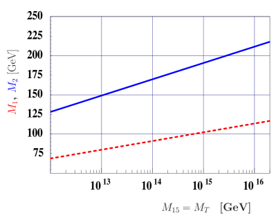
We can estimate the soft mass parameters given the above formulas for a given choice of and . We show some arbitrarily chosen examples in fig. (1). Note that the result shown is approximate, since we are (a) using the leading log approximation and (b) two loop effects are numerically important, especially for , but not included. The figure serves to show that for any the resulting mass parameters are always smaller than the mSugra expectations for the same choice of initial parameters (). While the exact values depend on () and on the other mSugra parameters, this feature is quite generally true in all of the () plane. Note, that the running is different for the different scalar mass parameters, but the ratio of the gaugino mass parameters always stays close to the mSugra expectation, .
|
III Numerical results
In this section we discuss our numerical results. All the plots shown below are based on the program packages SPheno Porod:2003um and micrOMEGAs Belanger:2004yn ; Belanger:2006is . We use SPheno V3 PorodWebpage , including the RGEs for the + case Rossi:2002zb ; Hirsch:2008gh at the 2-loop level for gauge couplings and gaugino masses and at one-loop level for the remaining MSSM parameters and the 15-plet parameters, for a discussion see Hirsch:2008gh . For any given set of mSugra and 15-plet parameters SPheno calculates the supersymmetric particle spectrum at the electro-weak scale, which is then interfaced with micrOMEGAs2.2 micrOMEGAsWebpage to calculate the relic density of the lightest neutralino, .
For the standard model parameters we use the PDG 2008 values PDG2008 , unless specified otherwise. As discussed below, especially important are the values (and errors) of the bottom and top quark masses, GeV and GeV. Note, the is understood to be the pole-mass and is the mass. As the allowed range for we always use the 3 c.l. boundaries as given in PDG2008 , i.e. . Note, however that the use of 1 contours results in very similar plots, due to the small error bars.
|
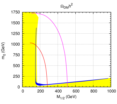
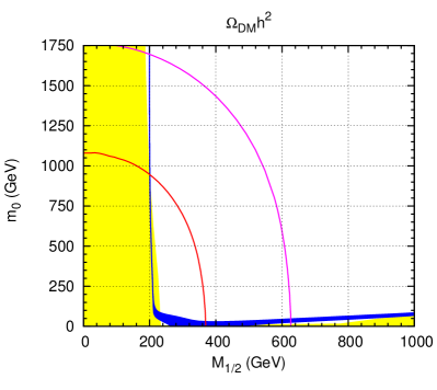
|
In the “seesaw sector” we have the parameters connected with the 15-plets, i.e. , , and . For the calculation of the dark matter abundance the most important parameter is . It has turned out that the effects of , and on the relic abundance of neutralinos are very minor. Note, however, that as discussed in the previous section, atmospheric neutrino oscillation data can not be explained in our setup, if the triplet mass is larger than approximately GeV. Also, the non-observation of lepton flavour violating (LFV) decays puts an upper bound on . The latter, however, is strongly dependent on and depends also on and . We will first show results using different values of as free parameter, without paying attention to neutrino masses and LFV. We will discuss how our results change for correctly fitted neutrino masses and angles towards the end of this section, where we also discuss and compare LFV excluded regions with DM allowed ones.
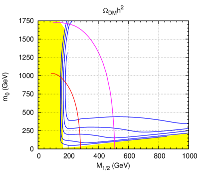
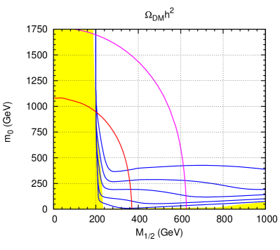
We define our “standard choice” of mSugra parameters as , and and use these values in all plots, unless specified otherwise. We then show our results in the plane of the remaining two free parameters, (). Fig. (2) shows in the top panel contours of equal dark matter density, . The lines are constant with . In the bottom panel we show the range of parameters allowed by the DM constraint at 3 c.l. In both cases, to the left a pure mSugra calculation, whereas the plot to the right shows mSugra + 15-plet with GeV. In each plot the yellow regions are eluded either by the lighter scalar tau being the LSP (to the bottom right) or by the LEP limit on the mass of the lighter chargino (to the left), GeV. In addition, we show two lines of constant lightest Higgs boson mass, GeV (dotted) and GeV (dashed), as calculated by SPheno, see the discussion below.
The plots show three of the different allowed regions discussed in the introduction. To the right the co-annihilation region, here the lightest neutralino and the lighter scalar tau are nearly degenerate in mass. The line going nearly vertically upwards at constant is the “focus point” line. The small region connecting the two lines are the remains of the bulk region, which has shrunk considerably due to the reduced error bars on after the most recent WMAP data Komatsu:2008hk . The focus point line is excluded by the LEP constraint on the lighter chargino mass at low and moderate values of . It becomes allowed only at values of larger than (very roughly) 1-1.5 TeV. However, note that the exact value of at which the focus point line becomes allowed is extremely sensitive to errors in , both from the experimental bound and the error in the theoretical calculation.
Comparing the results for the pure mSugra case to the mSugra+15-plet calculation, two differences are immediately visible in fig. (2). First, the focus point line is shifted towards larger values of . This is due to the fact that for the 15-plet at GeV the neutralino is lighter than in the mSugra case at the same value of , compare to fig. (1). Maintaining the same relation between and as in the mSugra case requires a then a larger value of . Note that for the same reason the excluded region from the LEP bound on the chargino mass is larger than in the mSugra case. Second on finds that the co-annihilation line is shifted towards smaller values of . The latter can be understood from fig. (3).

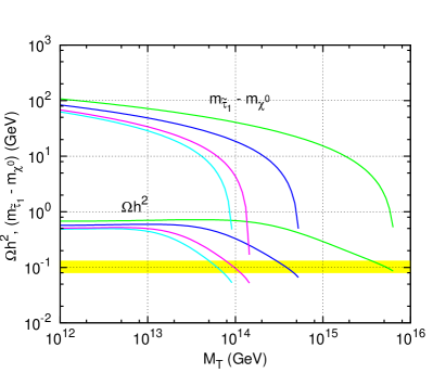
|
Fig. (3) shows the allowed region for the dark matter density in the () plane for our “standard choice” of other mSugra parameters for a number of different (to the left). The plot shows how the co-annihilation line moves towards smaller values of for smaller values of . The plot on the right in fig. (3) explains this behaviour. It shows the variation of the mass difference (top lines) and of (bottom lines), as a function of for four different values of : 0 (cyan), 50 (magenta), 100 (blue) and 150 GeV (green) for one fixed value of GeV. The yellow region corresponds to the experimentally allowed DM region. Co-annihilation requires a small value of , typically smaller than a few GeV. With decreasing values of the gaugino masses run down to smaller values faster than the slepton masses, thus effectively increasing in these examples with respect to mSugra. To compensate for this effect at constant smaller values of are required to get the in the required range.
At this point a short discussion of the Higgs boson mass bound might be in order. LEP excluded a light Higgs boson with SM couplings with masses below GeV PDG2008 . For reduced coupling of the Higgs boson to the bound is less severe, so this bound is not strictly valid in all of MSSM space. More important for us, however, is the theoretical uncertainty in the calculation of the lightest Higgs boson mass. SPheno calculates at two-loop level using renormalization. Expected errors for this kind of calculation, including a comparison of different public codes, have been discussed in Allanach:2004rh . As discussed in Allanach:2004rh ; Heinemeyer:2004xw even at the 2-loop level uncertainties in the calculation of can be of the order of GeV. In this context it is interesting to note that FeynHiggs Frank:2006yh , which calculates the higgs masses in a diagrammatic approach within the renormalization scheme tends to predict higgs masses which are systematically larger by GeV, when compared with the calculation. We therefore showed in fig. (2) two lines of constant Higgs boson masses. The value of GeV is taking the LEP bound at face value, while the lower value of GeV estimates the parameter region which is excluded conservatively, including the theoretical error. Since the lightest Higgs boson mass varies slowly with and , even a relatively tiny change in of, say 1 GeV, shifts the extreme values of the excluded region by GeV in (at small ) and by GeV in (at small ).
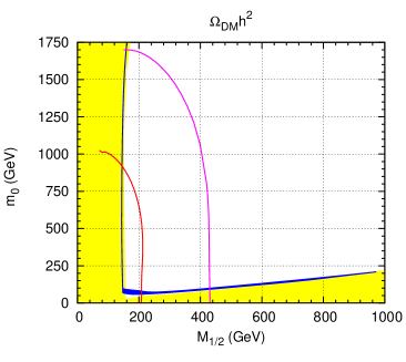 |
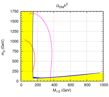 |
Moreover, it is well known that the calculated Higgs boson masses are strongly dependent on the mixing in the stop sector and thus, indirectly, on the value of . This is shown for the case of a pure mSugra calculation in fig. (4). Here we show two examples for the DM allowed region and the regions disfavoured by the Higgs boson mass bound at GeV and GeV. Larger negative leads to a less stringent constraint (for ). Note, that all of the bulk region becomes allowed at GeV, once the theoretical uncertainty in the Higgs boson mass calculation is taken into account. We have checked for a few values of that for the case of mSugra+ the resulting Higgs boson bounds are very similar. We thus do not repeat the corresponding plots here. Comparing the calculations shown in fig. (4) and the mSugra calculation in fig. (2) with each other, one finds that the DM allowed regions are actually affected very little by the choice of . We have checked that this is also the case for mSugra + seesaw type-II.
 |
 |
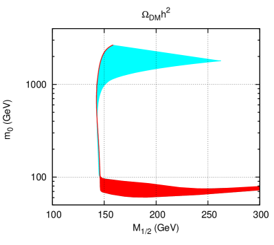
As mentioned above the uncertainty in the top mass is important for the calculation of the relic density. At low and moderate values of the exact value of affects mainly the focus point region. As fig. (2) demonstrates near the focus point line the relic density changes very abruptly even for tiny changes of . This is because a comparatively small value of is required to get a sufficiently enhanced coupling of the neutralino to the boson. In mSugra the value of is determined from all other parameters by the condition of having correct electro-weak symmetry breaking (EWSB) and usually leads to . In the focus point region varies abruptly, points to the “left” of the focus point region are usually ruled out by the fact that EWSB can not be achieved. Since is the largest fermion mass, its exact value influences the value of required to achieve EWSB most. The change of with respect to a change of then can lead to a significant shift in the DM allowed region of parameter space. This is demonstrated in fig. (5), which shows a zoom into the focus point region for pure mSugra (to the left) and mSugra + (to the right). The variation of the top mass shown corresponds to the current 1 allowed range PDG2008 . The pure mSugra is especially sensitive to a change of . At large values of the uncertainty in “fixing” from the DM constraint can be larger than GeV in the case of mSugra. Given this large uncertainty it would be impossible at present to distinguish the pure mSugra case from mSugra + seesaw, if the focus point region is the correct explanation of the observed DM. Note, however, that in the future the top mass will be measured more precisely. At the LHC one expects an uncertainty of 1-2 GeV Aad:2009wy at a linear collider could be determined down to an uncertainyy of MeV AguilarSaavedra:2001rg .
We now turn to a discussion of large . At large values of the width of the CP-odd Higgs boson becomes large, , and a wide s-channel resonance occurs in the region . The enhanced annihilation cross section reduces to acceptable levels, the resulting region is known as the “higgs funnel” region. In fig. (6) we show the allowed range of parameters in the () plane for one specific value of and three different values of . As demonstrated, the higgs funnel region is very sensitive to the choice of . It is fairly obvious that varying one can cover nearly all of the plane, even for fixed values of all other parameters. We have calculated the DM allowed region for various values of and found that the funnel appears for all , approximately.
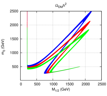
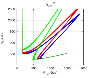
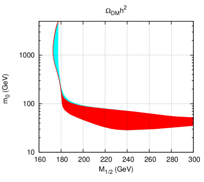
The strong dependence of the higgs funnel region on unfortunately does not imply automatically that if large is realized in nature one could get a very sensitive indirect “measurement” of the seesaw scale by determining (). The reason is that the higgs funnel is also very sensitive to the exact value of and to the values (and errors) of the top and bottom quark mass. The latter is demonstrated in fig. (7), where we show the DM allowed range of parameters for a fixed choice of and varying to the left (to the right) () within their current 1 c.l. error band. The position of the funnel is especially sensitive to the exact value of . Comparing fig. (7) with fig. (6) one can see that the uncertainty in and currently severely limit any sensitivity one could get on . However, future determinations of and could improve the situation considerably. For future uncertainties in see the discussion above for the focus point region. For reference Brambilla:2004wf estimates that could be fixed to GeV, which might even be improved to an accuracy of MeV according to Chetyrkin:2009fv .
|
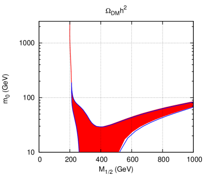
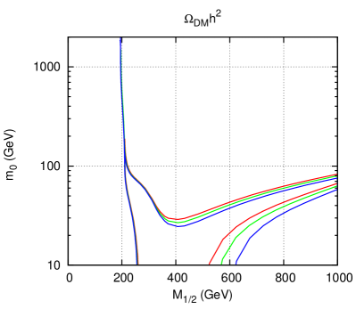
All of the above figures have been calculated using fixed values for and and negligibly small Yukawa couplings . This choice in general does not affect the calculation of the DM allowed regions much. However, a fully consistent calculation can not vary , and independently, since this will lead to neutrino masses and angles outside the experimentally allowed ranges. Since is diagonalized by the same matrix as the effective neutrino mass matrix, , see the previous section, the measured neutrino angles provide constraints on the relative size of the entries in . The absolute size of is then fixed for any fixed choice of and , once the neutrino spectrum is chosen to be hierarchical or quasi-degenerate. In the numerical calculation shown in fig. (8) we have chosen neutrino masses to be of the normal hierarchical type and fitted the neutrino angles to exact tri-bimaximal (TBM) values Harrison:2002er , i.e. , and . This has to be done in a simple iterative procedure, since the triplet parameters are defined at the high scale, whereas neutrino masses and angles are measured at low scale. For more details on the fit procedure see Hirsch:2008gh .
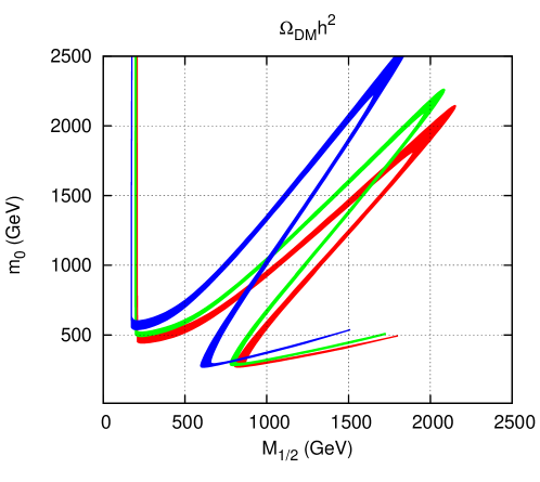
In fig. (8) to the left we show two calculations of the DM allowed regions. The allowed range for negligibly small neutrino Yukawa couplings is shown by the filled (red) region, while the calculation with fitted to correctly explain solar and atmospheric neutrino data is the one inside the (blue) lines. Note the logarithmic scale. As demonstrated, the exact values of are of minor importance for the determination of the parameter region allowed by the DM constraint. Slightly larger differences between the fitted and unfitted calculations are found pushing to larger values (see, however, below). For smaller values of , the entries in needed to correctly explain neutrino data are smaller and, thus, affects the DM allowed region even less for GeV.
In fig. (8) to the right we compare three different calculations for , (red), (green) and (blue), for fixed choice of other parameters. This plot serves to show that also the exact choice of is of rather minor importance for the determination of the DM allowed region. Very similar results have been found for , we therefore do not repeat plots varying here.
|
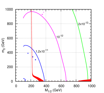
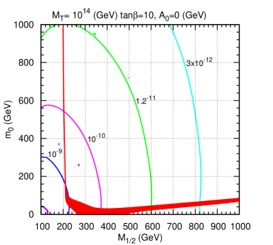
Finally, we will compare the constraints imposed on the parameter space of the model by with the constraints from the current data on non-observation of lepton flavour violating processes. Since LFV within the present model has been studied in some detail in Hirsch:2008gh , we will not repeat all of the discussion here. Instead, here we concentrate on exclusively, since the upper bound on of PDG2008 has been shown to provide currently the most important constraint.
In fig. (9) we show the DM allowed parameter regions for and two values of , GeV (to the left) and GeV (to the right), for a fixed choice of all other parameters. Superimposed on this plot are lines of constant branching ratio for . The latter have been calculated requiring neutrino masses being hierarchical and fitted to solar and atmospheric neutrino mass squared differences and neutrino angles fitted to TBM values. Within the () region shown, can vary by two orders of magnitude, depending on the exact combination of (), even for all other parameters fixed. The most important parameter determining , once neutrino data is fixed, however, is , as can be seen comparing the figure to the left with the plot on the right. While for GeV about “half” of the plane is ruled out by the non-observation of , for GeV with the current upper limit nearly all of the plane becomes allowed. The strong dependence of on can be understood from the analytical formulas presented in Hirsch:2008gh . In this paper it was shown that scales very roughly as , if neutrino masses are to be explained correctly. For one thus concludes that with present data values of larger than (few) GeV - (few) GeV are excluded by , to be compared with GeV from the measured neutrino masses. Note, however, that (i) the constraint from neutrino masses is relatively independent of , and , while shows strong dependence on these parameters; and (ii) allowing the value of the reactor angle to vary up to its experimental upper limit, Maltoni:2004ei , leads to larger values of and thus to a tighter upper limit on .
 |
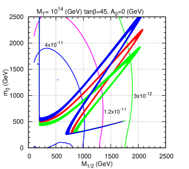 |
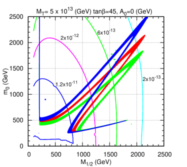
In fig. (10) we show the results for a calculation comparing dark matter and LFV in the case of large . Here the same constraints as in fig. (9) are shown, however for . Again we show the calculation for two values of , since is the most important free parameter. It is known that at large values of , LFV decays are enhanced due to an enhanced chargino diagram, which in the limit of large scales approximately as Hisano:1995cp . Therefore, constraints on the parameter space from non-observation of LFV decays are more severe in case of large , leading to tighter upper limits on . This is clear if we compare fig. (9) and fig. (10), noticing the different scales. However, because of the higgs funnel region developing for large , the interesting part of the parameter space enlarges compensating for the larger values of the LFV decays. This can be seen in fig. (10), where for GeV (left), most of the () plane is allowed by the upper limit on , while for GeV (right), about “half” of the plane is ruled out by this limit.
We have concentrated in this paper on discussing DM in mSugra with a seesaw type-II. Before closing this section, we would like to briefly comment on the case of seesaw type-I. In seesaw type-I one adds two or more singlet superfields to the superpotential of the MSSM. These singlets have Yukawa couplings to the standard model lepton doublet and a Majorana mass term, but no other couplings to any of the MSSM fields. The running of the mSugra soft parameters in this setup is therefore only changed by the neutrino Yukawa couplings. Just as in the seesaw type-II one can estimate from current neutrino data that the Yukawa couplings are order for the right-handed Majorana mass order GeV. 333Different from the seesaw type-II, where depends linearly on , however, in seesaw type-I Yukawas scale like . For any smaller than this number, one therefore expects that the running of the soft parameters is essentially mSugra-like. (Apart from small off-diagonal terms in , which are exactly zero in mSugra.) This implies that also the DM regions should be very close to those found in the mSugra case. We have confirmed this expectation by calculating the DM allowed region for our standard choice of mSugra parameters and various values of the right-handed neutrino masses. Even for at the upper limit allowed by perturbativity we did not find any significant departure from the mSugra case. With the hindsight of the results shown in fig. (8) for the seesaw type-II this is not surprising.
One exceptional case for the seesaw type-I has been discussed, however, recently in Kadota:2009vq . The authors of Kadota:2009vq observed that for Yukawa couplings close to one and a large value of the common trilinear , say GeV, the left sneutrinos can be the next-to-LSP (NLSP) for small-to-moderate values of , and . For a sneutrino NLSP nearly degenerate with the lightest neutralino a new co-annihilation regions then shows up at small values of . We have repeated this calculation with three right-handed neutrinos (Kadota:2009vq use only one singlet superfield) and confirm the sneutrino co-annihilation region for and large . However, in our calculation, if we insist on fitting the large atmospheric and solar angles, all of the region is excluded by upper limits on LFV decays, if we put the matrix of the Casas-Ibarra parameterization for the neutrino Yukawa couplings Casas:2001sr to the identity matrix. As has been shown in Ellis:2002fe ; Arganda:2005ji , we could, in principle, avoid these strong constraints from LFV by a careful adjustments of the unknown parameters in . We did, however, not attempt to do a systematic study as to how has to be chosen that the sneutrino co-annihilation becomes consistent with LFV decays.
IV Conclusions
In conclusion, we have calculated the neutralino relic density in a supersymmetric model with mSugra boundary conditions including a type-II seesaw mechanism to explain current neutrino data. We have discussed how the allowed ranges in mSugra parameter space change as a function of the seesaw scale. The stau co-annihilation region is shifted towards smaller for smaller values of the triplet mass , while the bulk region and the focus point line are shifted towards larger values of for sufficiently below the GUT scale. The higgs funnel, which appears at large values of has turned out to be especially sensitive to the value of . Determining from the mass of any gaugino and from a sparticle which is not important for the DM calculation, one could, therefore, get a constraint on from the requirement that the observed is correctly explained by the calculated .
On the positive side, we can remark that current data on neutrino masses put an upper bound on of the order of GeV. Since this is at least one order of magnitude smaller than the GUT scale, the characteristic shifts in the DM regions are necessarily non-zero if our setup is the correct explanation of the observed neutrino oscillation data. Even more stringent upper limits on follow, in principle, from the non-observation of LFV decays. A smaller implies larger shifts of the DM region. However, the “exact” upper limit on from LFV decays depends strongly on , and , and thus can be quantified only once at least some information on these parameters is available.
On the down side, we need to add a word of caution. We have found that the DM calculation suffers from a number of uncertainties, even if we assume the soft masses to be perfectly known. The most important SM parameters turn out to be the bottom and the top quark mass. The focus point line depends extremely sensitively on the exact value of the top mass, the higgs funnel shows a strong sensitivity on both, and .
Finally, it is clear that quite accurate sparticle mass measurements will be necessary, before any quantitative conclusions can be taken from the effects we have discussed. Unfortunately, such accurate mass measurements might be very difficult to come by for different reasons. In the focus point region all scalars will be heavy, leading to small production cross section at the LHC. In the co-annihilation line with a nearly degenerate stau and a neutralino, the stau decays produce very soft taus, which are hard for the LHC to measure. And the higgs funnel extends, depending on and , to very large values of (), at least partially outside the LHC reach. Nevertheless, DM provides in principle an interesting constraint on the (supersymmetric) seesaw explanation of neutrino masses, if seesaw type-II is realized in nature, a fact which to our knowledge has not been discussed before in the literature.
Acknowledgements
Work supported by Spanish grants FPA2008-00319/FPA and Accion Integrada HA-2007-0090 (MEC). The work of J.N.E.. is supported by Fundação para a Ciência e a Tecnologia under the grant SFRH/BD/29642/2006. The work of J.C.R. and J.N.E. is also supported by the RTN Network MRTN-CT-2006-035505 and by Fundação para a Ciência e a Tecnologia through the projects CFTP-FCT UNIT 777 and CERN/FP/83503/2008. W.P. is partially supported by the German Ministry of Education and Research (BMBF) under contract 05HT6WWA and by the DAAD project number D/07/13468.
References
- (1) G. Jungman, M. Kamionkowski and K. Griest, Phys. Rept. 267, 195 (1996) [arXiv:hep-ph/9506380].
- (2) G. Bertone, D. Hooper and J. Silk, Phys. Rept. 405, 279 (2005) [arXiv:hep-ph/0404175].
- (3) C. Amsler et al., Physics Letters B667, 1 (2008); http://pdg.lbl.gov/
- (4) D. N. Spergel et al. [WMAP Collaboration], Astrophys. J. Suppl. 148, 175 (2003) [arXiv:astro-ph/0302209].
- (5) E. Komatsu et al. [WMAP Collaboration], Astrophys. J. Suppl. 180, 330 (2009) [arXiv:0803.0547 [astro-ph]].
- (6) M. Tegmark et al. [SDSS Collaboration], Phys. Rev. D 74, 123507 (2006) [arXiv:astro-ph/0608632].
- (7) L. Bergstrom, arXiv:0903.4849 [hep-ph].
- (8) H. Baer, E. K. Park and X. Tata, arXiv:0903.0555 [hep-ph].
- (9) Y. Fukuda et al. [Super-Kamiokande Collaboration], Phys. Rev. Lett. 81, 1562 (1998)
- (10) SNO, Q. R. Ahmad et al., Phys. Rev. Lett. 89, 011301 (2002), [nucl-ex/0204008].
- (11) KamLAND, K. Eguchi et al., Phys. Rev. Lett. 90, 021802 (2003), [hep-ex/0212021].
- (12) [MINOS Collaboration], arXiv:0708.1495 [hep-ex].
- (13) KamLAND Collaboration, arXiv:0801.4589 [hep-ex].
- (14) For a review of neutrino oscillation data, see: M. Maltoni, T. Schwetz, M. A. Tortola and J. W. F. Valle, New J. Phys. 6, 122 (2004); an updated analysis has now been published in T. Schwetz, M. Tortola and J. W. F. Valle, New J. Phys. 10, 113011 (2008) [arXiv:0808.2016 [hep-ph]] where all experimental references can be found.
- (15) P. F. Harrison, D. H. Perkins and W. G. Scott, Phys. Lett. B530, 167 (2002), [hep-ph/0202074].
- (16) S. Weinberg, Phys. Rev. Lett. 43, 1566 (1979); S. Weinberg, Phys. Rev. D 22, 1694 (1980).
- (17) E. Ma, Phys. Rev. Lett. 81, 1171 (1998) [arXiv:hep-ph/9805219].
- (18) P. Minkowski, Phys. Lett. B 67 (1977) 421.
- (19) T. Yanagida, in KEK lectures, ed. O. Sawada and A. Sugamoto, KEK, 1979; M Gell-Mann, P Ramond, R. Slansky, in Supergravity, ed. P. van Niewenhuizen and D. Freedman (North Holland, 1979);
- (20) R.N. Mohapatra and G. Senjanovic, Phys. Rev. Lett. 44 912 (1980).
- (21) J. Schechter and J. W. F. Valle, Phys. Rev. D 22, 2227 (1980).
- (22) T. P. Cheng and L. F. Li, Phys. Rev. D 22, 2860 (1980).
- (23) R. Foot, H. Lew, X. G. He and G. C. Joshi, Z. Phys. C 44, 441 (1989).
- (24) F. Borzumati and A. Masiero, Phys. Rev. Lett. 57, 961 (1986).
- (25) J. Hisano, T. Moroi, K. Tobe, M. Yamaguchi and T. Yanagida, Phys. Lett. B 357, 579 (1995) [arXiv:hep-ph/9501407].
- (26) J. Hisano, T. Moroi, K. Tobe and M. Yamaguchi, Phys. Rev. D 53, 2442 (1996) [arXiv:hep-ph/9510309].
- (27) J. R. Ellis, J. Hisano, M. Raidal and Y. Shimizu, Phys. Rev. D 66, 115013 (2002) [arXiv:hep-ph/0206110].
- (28) F. Deppisch, H. Pas, A. Redelbach, R. Ruckl and Y. Shimizu, Eur. Phys. J. C 28, 365 (2003) [arXiv:hep-ph/0206122].
- (29) E. Arganda and M. J. Herrero, Phys. Rev. D 73, 055003 (2006) [arXiv:hep-ph/0510405].
- (30) S. Antusch, E. Arganda, M. J. Herrero and A. M. Teixeira, JHEP 0611, 090 (2006) [arXiv:hep-ph/0607263].
- (31) E. Arganda, M. J. Herrero and A. M. Teixeira, JHEP 0710, 104 (2007) [arXiv:0707.2955 [hep-ph]].
- (32) A. Rossi, Phys. Rev. D 66, 075003 (2002) [arXiv:hep-ph/0207006].
- (33) M. Hirsch, S. Kaneko and W. Porod, Phys. Rev. D 78, 093004 (2008) [arXiv:0806.3361 [hep-ph]].
- (34) J. Hisano, M. M. Nojiri, Y. Shimizu and M. Tanaka, Phys. Rev. D 60, 055008 (1999) [arXiv:hep-ph/9808410].
- (35) N. V. Krasnikov, Phys. Lett. B 388 (1996) 783 [arXiv:hep-ph/9511464].
- (36) N. Arkani-Hamed, H. C. Cheng, J. L. Feng and L. J. Hall, Phys. Rev. Lett. 77 (1996) 1937 [arXiv:hep-ph/9603431].
- (37) D. Nomura, Phys. Rev. D 64 (2001) 075001 [arXiv:hep-ph/0004256].
- (38) W. Porod and W. Majerotto, Phys. Rev. D 66 (2002) 015003 [arXiv:hep-ph/0201284].
- (39) F. Deppisch, H. Pas, A. Redelbach, R. Ruckl and Y. Shimizu, Phys. Rev. D 69 (2004) 054014 [arXiv:hep-ph/0310053].
- (40) F. del Aguila et al., Eur. Phys. J. C 57 (2008) 183 [arXiv:0801.1800 [hep-ph]].
- (41) F. Deppisch, H. Pas, A. Redelbach and R. Ruckl, Phys. Rev. D 73, 033004 (2006) [arXiv:hep-ph/0511062].
- (42) A. Bartl, K. Hidaka, K. Hohenwarter-Sodek, T. Kernreiter, W. Majerotto and W. Porod, Eur. Phys. J. C 46, 783 (2006) [arXiv:hep-ph/0510074].
- (43) M. Hirsch, J. W. F. Valle, W. Porod, J. C. Romao and A. Villanova del Moral, Phys. Rev. D 78, 013006 (2008) [arXiv:0804.4072 [hep-ph]].
- (44) E. Carquin, J. Ellis, M. E. Gomez, S. Lola and J. Rodriguez-Quintero, arXiv:0812.4243 [hep-ph].
- (45) J. N. Esteves, J. C. Romao, A. Villanova del Moral, M. Hirsch, J. W. F. Valle and W. Porod, JHEP 05 (2009) 003 [arXiv:0903.1408]
- (46) G. A. Blair, W. Porod and P. M. Zerwas, Eur. Phys. J. C27, 263 (2003), [hep-ph/0210058].
- (47) A. Freitas, W. Porod and P. M. Zerwas, Phys. Rev. D72, 115002 (2005), [hep-ph/0509056].
- (48) M. R. Buckley and H. Murayama, Phys. Rev. Lett. 97, 231801 (2006) [arXiv:hep-ph/0606088].
- (49) J. R. Ellis, J. S. Hagelin, D. V. Nanopoulos, K. A. Olive and M. Srednicki, Nucl. Phys. B 238, 453 (1984).
- (50) K. Griest and D. Seckel, Phys. Rev. D 43, 3191 (1991).
- (51) M. Drees and M. M. Nojiri, Phys. Rev. D 47, 376 (1993) [arXiv:hep-ph/9207234].
- (52) G. B. Gelmini and P. Gondolo, Phys. Rev. D 74, 023510 (2006) [arXiv:hep-ph/0602230].
- (53) B. C. Allanach, G. Belanger, F. Boudjema and A. Pukhov, JHEP 0412, 020 (2004) [arXiv:hep-ph/0410091].
- (54) H. Baer, C. Balazs and A. Belyaev, JHEP 0203, 042 (2002) [arXiv:hep-ph/0202076].
- (55) J. L. Feng, K. T. Matchev and T. Moroi, Phys. Rev. D 61, 075005 (2000) [arXiv:hep-ph/9909334].
- (56) K. Kadota, K. A. Olive and L. Velasco-Sevilla, arXiv:0902.2510 [hep-ph].
- (57) For reviews on mSugra and MSSM, see for example: H. P. Nilles, Phys. Rept. 110, 1 (1984). H. E. Haber and G. L. Kane, Phys. Rept. 117, 75 (1985); S. P. Martin, arXiv:hep-ph/9709356.
- (58) S. P. Martin and M. T. Vaughn, Phys. Rev. D 50, 2282 (1994) [Erratum-ibid. D 78, 039903 (2008)] [arXiv:hep-ph/9311340].
- (59) W. Porod, Comput. Phys. Commun. 153, 275 (2003) [arXiv:hep-ph/0301101];
- (60) G. Belanger, F. Boudjema, A. Pukhov and A. Semenov, Comput. Phys. Commun. 176, 367 (2007) [arXiv:hep-ph/0607059].
- (61) G. Belanger, F. Boudjema, A. Pukhov and A. Semenov, Comput. Phys. Commun. 174, 577 (2006) [arXiv:hep-ph/0405253].
- (62) The latest version of SPheno can be obtained from: http://theorie.physik.uni-wuerzburg.de/ porod/SPheno.html
- (63) http://wwwlapp.in2p3.fr/lapth/micromegas/
- (64) B. C. Allanach, A. Djouadi, J. L. Kneur, W. Porod and P. Slavich, JHEP 0409, 044 (2004) [arXiv:hep-ph/0406166].
- (65) S. Heinemeyer, W. Hollik, H. Rzehak and G. Weiglein, Eur. Phys. J. C 39 (2005) 465
- (66) M. Frank, T. Hahn, S. Heinemeyer, W. Hollik, H. Rzehak and G. Weiglein, JHEP 0702, 047 (2007) [arXiv:hep-ph/0611326]. The FeynHiggs code can be found at: http://www.feynhiggs.de/
- (67) G. Aad et al. [The ATLAS Collaboration], arXiv:0901.0512 [hep-ex].
- (68) J. A. Aguilar-Saavedra et al. [ECFA/DESY LC Physics Working Group], arXiv:hep-ph/0106315.
- (69) N. Brambilla et al. [Quarkonium Working Group], arXiv:hep-ph/0412158.
- (70) K. G. Chetyrkin, J. H. Kuhn, A. Maier, P. Maierhofer, P. Marquard, M. Steinhauser and C. Sturm, arXiv:0907.2110 [hep-ph].
- (71) J. A. Casas and A. Ibarra, Nucl. Phys. B618, 171 (2001), [hep-ph/0103065].