Abstract

We study two-dimensional ${\cal N}=(2,2)$ $SU(N)$ super Yang-Mills theory on Euclidean two-torus using Sugino’s lattice regularization. We perform the Monte-Carlo simulation for $N=2,3,4,5$ and then extrapolate the result to $N=\infty$. With the periodic boundary conditions for the fermions along both circles, we establish the existence of a bound state in which scalar fields clump around the origin, in spite of the existence of a classical flat direction. In this phase the global $({\mathbb{Z}}_{N})^{2}$ symmetry turns out to be broken. We provide a simple explanation for this fact and discuss its physical implications.

1 Introduction

Large-$N$ supersymmetric Yang-Mills theories (SYM) are promising candidates for nonperturbative formulations of the superstring theories [1, 2, 3, 4, 5]. Recent developments of discretization technique enable us to study nonperturbative aspects of these theories. (For a recent review, see e.g. [6, 7].) Especially, one-dimensional maximally supersymmetric gauge theory has been studied extensively [8, 9, 10, 11, 12] and the gauge/gravity duality [4, 5] has been confirmed very precisely, including the stringy $\alpha^{\prime}$ corrections [12]. By assuming that the gauge/gravity duality holds, then the Monte-Carlo simulation of the gauge theory provides a new and powerful tool to study the physics of black holes.

Next simplest model to study is two-dimensional theory, of which some lattice regularizations are known. Maximally supersymmetric 2d SYM is expected to have dual D1-brane description in type IIB superstring theory [5]. By compactifying the spatial direction, one obtains D1-branes winding on the compactified direction. By taking T-dual, one obtains a system of D0-branes in compact space, which can have several phases – if D0-branes are smeared along the compactified direction it is a black string, and if they are localized in a small region it is a black hole. The transition between these phases (the Gregory-Laflamme transition [13]) corresponds to the breakdown of the global ${\mathbb{Z}}_{N}$ symmetry in the gauge theory [14]. By studying the Gregory-Laflamme transition in supergravity and then by using the gauge/gravity duality to translate the supergravity to the gauge theory, one can study the phase structure of the gauge theory at strong coupling [15]. Using the duality in the opposite direction, we can study the detail of the stringy correction to the Gregory-Laflamme transition with the Monte-Carlo simulation of the gauge theory. At present, it is difficult to study the maximally supersymmetric 2d SYM by using the Monte-Carlo simulation. However, four-supercharge system has been studied extensively by using the formulations free from fine tuning.

In this paper, we study two-dimensional ${\cal N}=(2,2)$ $SU(N)$ SYM on two-torus using Sugino’s lattice regularization [16]. In this model, the restoration of supersymmetry without fine-tuning has been tested extensively [18]. We study $N=2,3,4,5$ and extrapolate to the planar limit $N=\infty$. The action in the continuum is obtained from 4d ${\cal N}=1$ SYM through the dimensional reduction, and is given by

$$S=N\int_{0}^{L_{x}}dx\int_{0}^{L_{y}}dy\ \mathop{Tr}\nolimits\left\{\frac{1}{4}F_{\mu\nu}^{2}+\frac{1}{2}(D_{\mu}X_{i})^{2}-\frac{1}{4}[X_{i},X_{j}]^{2}-\frac{i}{2}\bar{\psi}\Gamma^{\mu}D_{\mu}\psi-\frac{1}{2}\bar{\psi}\Gamma^{i}[X_{i},\psi]\right\},$$ (1)

where $\mu$ and $\nu$ run $x$ and $y$, $i$ and $j$ run $1$ and $2$, and $\Gamma^{I}=(\Gamma^{\mu},\Gamma^{i})$ are gamma matrices in four dimensions. $X_{i}$ are $N\times N$ hermitian matrices, $\psi_{\alpha}$ are $N\times N$ fermionic matrices with a Majorana index $\alpha$ and the covariant derivative is given by $D_{\mu}=\partial_{\mu}-i[A_{\mu},\ \cdot\ ]$. The only parameters of the model are the size of circles $L_{x}$ and $L_{y}$. (Note that the coupling constant can be absorbed by redefining the fields and coordinates. In other words, the ’t Hooft coupling $\lambda$ which has mass dimension $2$ can be taken to be $\lambda=1$. Then the strong coupling corresponds to the large volume.) There are several motivations to study this system. Firstly, it is the simplest SYM in two dimensions which can be studied nonperturbatively by lattice simulation. Especially, notorious “sign problem” is absent. Secondly, we can expect that it is qualitatively similar to maximally supersymmetric (${\cal N}=(8,8)$) SYM, which is conjectured to be dual to type II superstring. Thirdly, its bosonic cousin is studied in [24] and it is interesting to compare the phase structure. In the bosonic model, the ${\mathbb{Z}}_{N}$ symmetry is broken below the critical volume. In the supersymmetric model it is expected to be broken in any finite volume [25]. The argument in [25] is valid only large and small volume region and it is desirable to check the breakdown of ${\mathbb{Z}}_{N}$ at intermediate volume.

An obstacle for the simulation is the existence of the flat direction, along which two scalar fields $X_{1}$ and $X_{2}$ commute. In contrary to a theory on ${\mathbb{R}}^{1,3}$, there is no superselection of the moduli parameter in this case. That is, eigenvalues of scalars are determined dynamically. Therefore, some mechanism which restrict eigenvalues to a finite region is necessary in order for the stable simulation. One possible way is to introduce an IR regulator and gradually remove it. In [18, 21, 22] this method has been applied to the $SU(2)$ theory at finite temperature. In those works, a mass term of scalars has been introduced and physical quantities are evaluated by an extrapolation to the massless limit or evaluated with small scalar mass. In this case, as we will see, in fact the scalar eigenvalues spread as IR regulator is removed. In string terminology, this phase can be understood as a gas of freely propagating D-branes.

At large-$N$, there is a more interesting phase, namely a bound state in which eigenvalues clump to a small region [25]. It is metastable at finite-$N$ and becomes stable at large-$N$. This bound state is a cousin of the one in one-dimensional system, which has been found in [9], and corresponds to the black brane background in type II superstring. (The black brane solution in supergravity corresponds to the bound state of the D-branes. Because the scalar fields represent the collective coordinates of the D-branes, the bunch of the D-branes is nothing but the bound state of scalar eigenvalues.) In this paper we study this phase. Because the very existence of this bound state is nontrivial from a purely field-theoretical point of view, we provide numerical evidence. As we will see, with periodic-periodic (P-P) boundary conditions for fermions, we construct the bound state explicitly. In this bound state, there are two possible phases, namely the $({\mathbb{Z}}_{N})^{2}$ broken and unbroken phases. (The model has global $({\mathbb{Z}}_{N})^{2}$ symmetry, which shifts the complex phases of Wilson loops winding on circles. If Wilson loops are non-zero, then the $({\mathbb{Z}}_{N})^{2}$ symmetry is spontaneously broken.) We study the phase structure under the variation of the periods. Because of the limitation of the resources, we study only the case of $L_{x}=L_{y}$. We confirm that, in the bound state, the $({\mathbb{Z}}_{N})^{2}$ symmetry is broken as discussed in [25]. With antiperiodic-periodic (A-P) boundary conditions, we need rather large $N$ to find such an bound state and we could not construct it numerically. Hence we cannot discuss the thermal properties of the black brane in this paper. However we can expect that we can study the finite temperature system in near future, by using a faster computer.

This paper is organized as follows. In § 2 we review the conjectured phase diagram and explain its physical implications. In § 3 we show the numerical results. We give the conclusion and discussion in § 4. The simulation details are explained in the appendices.

2 Conjectured phase structure

In this section we review the expectations on the phase structure. In short, the ${\mathbb{Z}}_{N}$ symmetry is broken in the bound state. The phases are summarized in Table 1.

Model	large volume	finite volume	small volume
4d $\mathcal{N}=1$, P-P	$(\mathbb{Z}_{N})^{4}$ and (broken)	$(\mathbb{Z}_{N})^{4}$ and (broken)	$(\mathbb{Z}_{N})^{4}$ and (broken)
2d $\mathcal{N}=(2,2)$, P-P	$(\mathbb{Z}_{N})^{2}$	(broken)	(broken)
2d $\mathcal{N}=(8,8)$, A-P	$\mathbb{Z}_{N}$	(phase transition(s))	(broken)

Table 1: Conjecture for phases of various super Yang-Mills. In this paper, we confirm the 2d $\mathcal{N}=(2,2)$ case numerically.

2.1 4d ${\cal N}=1$ SYM on Euclidean four-torus

Let us start by considering the 4d ${\cal N}=1$ SYM on four-torus $T^{4}$. For all circles we impose periodic boundary conditions for both bosons and fermions. Let $L_{\mu}\ (\mu=1,\cdots,4)$ be the periods along four directions and $W_{\mu}$ be the Wilson loops winding on each directions,

$$W_{\mu}=P\exp\left(i\int_{0}^{L_{\mu}}dx^{\mu}A_{\mu}\right),$$ (2)

where the contraction over $\mu$ is not taken in the right hand side. Under the global $({\mathbb{Z}}_{N})^{4}$ transformation, $W_{\mu}$ are multiplied by phase factors,

$$W_{\mu}\to e^{2\pi in_{\mu}/N}W_{\mu}\qquad(n_{\mu}\in{\mathbb{Z}}).$$ (3)

Therefore the $({\mathbb{Z}}_{N})^{4}$ is broken if $\mathop{Tr}\nolimits W_{\mu}$ have nonzero expectation values. In 4d ${\cal N}=1$, there are (at least) two phases – $({\mathbb{Z}}_{N})^{4}$ broken and unbroken. (Note that the ${\mathbb{Z}}_{N}$ symmetry can be broken only in the large-$N$ limit.)

The existence of the $({\mathbb{Z}}_{N})^{4}$ unbroken phase can be shown as follows [26]. Consider the situation in which one of the periods $L_{1}$ is much smaller than other three periods $L_{2},L_{3}$ and $L_{4}$. Then essentially we obtain SYM on ${\mathbb{R}}^{3}\times S^{1}$. If we take $L_{1}\ll\Lambda_{{\rm QCD}}^{-1}\ll L_{2},L_{3},L_{4}$, the effective potential of the Wilson line phase $\ln W_{1}$ can be calculated perturbatively and it gives exactly zero. By taking monopole and instanton effects [27] into account, it turns out that the eigenvalue of the Wilson line (the Wilson line phases) repel each other once they spread uniformly. Therefore, ${\mathbb{Z}}_{N}$-unbroken configuration is stable. This calculation itself is done in a specific limit, but due to the supersymmetry the same result should hold at any volume [26].

The $({\mathbb{Z}}_{N})^{4}$ broken phase can be found at small volume limit [25]. Suppose that $({\mathbb{Z}}_{N})^{4}$ is broken, or equivalently, the Wilson line phases clump in a small region around the origin. If the size of the phase distribution is small enough, then the system can be approximated by its zero-dimensional reduction. This model has been studied extensively. Especially, it is known to have a bound state of eigenvalues even though it has a flat direction classically, and the size of the eigenvalue distribution is known [28, 29, 30]. It is small enough so that the assumption that the system is described by the zero-dimensional reduction is correct. Therefore, a $({\mathbb{Z}}_{N})^{4}$ broken phase exists at small volume. We expect this phase persists at any finite volume due to the supersymmetry.

2.2 2d ${\cal N}=(2,2)$ SYM on two-torus

2d ${\cal N}=(2,2)$ SYM is obtained from 4d ${\cal N}=1$ through the dimensional reduction. When we take two circles in 4d theory to be small, in order for the dimensional reduction to work the ${\mathbb{Z}}_{N}$ symmetries along these circles must be broken. In such a phase Wilson line phases clump, so it corresponds to the bound state in 2d theory. Therefore, it is natural to assume that the bound state in 2d theory corresponds to $({\mathbb{Z}}_{N})^{4}$ broken phase in 4d theory. If this is the case, the $({\mathbb{Z}}_{N})^{2}$ symmetry of the 2d theory should be broken.

At large volume, $({\mathbb{Z}}_{N})^{2}$ symmetry should be restored. This is because $({\mathbb{Z}}_{N})^{2}$ is essentially continuous $U(1)^{2}$ symmetry at large-$N$ and hence at noncompact two-dimensional space it is unbroken according to the Coleman’s theorem.

In § 3, we will confirm the above statement by numerical simulation. The discussion above does not exclude an existence of a ${\mathbb{Z}}_{N}$ unbroken phase; see a remark in § 3.1.

2.3 2d ${\cal N}=(8,8)$ SYM : ${\mathbb{Z}}_{N}$ broken phase as a black hole

For 2d ${\cal N}=(8,8)$ SYM, there is a dual gravity interpretation. Here we consider the correspondence between thermal SYM and black branes in type II supergravity. First, let us briefly describe the SYM in terms of D-branes. We impose the antiperiodic boundary condition. for temporal direction (we take $y$ to be temporal direction). In this case, the bound state (i.e. a state in which scalar eigenvalues clump around the origin) is dual to the system of coincident $N$ D1-branes at finite temperature. The temperature $T$ is inverse of the $\beta\equiv L_{y}$. By taking T-duality along the spatial circle ($x$-direction), we obtain the system of $N$ D0-branes, sitting in the compactified spatial dimension of radius $(2\pi)^{2}/L_{x}$. The Wilson line phases correspond to the positions of the D0-branes along $x$-direction.

According to the gauge/gravity duality conjecture [5], at low temperature this system is well approximated by type II supergravity, and for fixed $\beta$ there is a first-order phase transition associated with the breakdown of the ${\mathbb{Z}}_{N}$ symmetry along $x$-direction [14, 15]. Below the critical value of the radius $L_{x,c}\sim\sqrt{\beta}$, ${\mathbb{Z}}_{N}$ is broken. Along the temporal direction, ${\mathbb{Z}}_{N}$ is conjectured to be broken at any nonzero temperature, that is, the system is always deconfined. For 1d system obtained by dimensional reduction from 2d $\mathcal{N}=(8,8)$ SYM it has been confirmed by using the Monte-Carlo simulation [9, 12, 11].

The physical interpretation of the ${\mathbb{Z}}_{N}$ breakdown in string theory is simple. In ${\mathbb{Z}}_{N}$ unbroken phase, D0-branes (Wilson line phases) fill the compact direction uniformly. It is a “uniform black string”. If ${\mathbb{Z}}_{N}$ is broken completely, D0-branes clump to a small region along compact direction; it is similar to the usual “black hole” (black 0-brane). This black hole is small at low temperature, and cannot wind on the spatial direction. At high temperature the black hole becomes large, and gradually fills the compact dimension, wraps on it and becomes the black string. At intermediate temperature the “nonuniform black string” may exist. In this phase, ${\mathbb{Z}}_{N}$ is broken and phases of the Wilson line is distributed nonuniformly, but still the density is nonzero everywhere.

In the high-temperature limit, fermions decouple and the system reduces to 1d bosonic Yang-Mills. In [31] this limit was studied by the Monte-Carlo simulation and it was found that the nonuniform black string phase exists indeed. By fixing the temperature and varying the size of the spatial circle, there are two phase transitions, namely between uniform and nonuniform black strings and between the nonuniform black string and the black hole. The orders of the transitions are of third and second order, respectively.

The situation is similar for $(p+1)$-dimensional SYM with 16 supercharges, in which the bound state is dual to a bunch of D$p$-branes. At low temperature we can analyze it using type II supergravity and $({\mathbb{Z}}_{N})^{p}$ symmetry broken/unbroken phases correspond to smeared D0-brane solution and black 0-brane solution. For detailed phase structure, see [32].

We emphasize again that the bound state of scalar eigenvalues is necessary for the black brane description. In order to understand this statement, let us remind that the black brane is the bound state of very large number of D-branes (indeed the gravity picture is valid in the large-$N$ limit, where $N$ is nothing but the number of D-branes). Because the scalar fields represent the collective coordinates of the D-branes, the bound state of the D-branes is exactly the bound state of scalar eigenvalues.

2.4 $\mathbb{Z}_{N}$ breakdown and volume (in)dependence

Before concluding this section, we argue general features of the large-$N$ volume independence.

In the large-$N$ limit, if the ${\mathbb{Z}}_{N}$ symmetry is not broken then the system is volume independent (Eguchi-Kawai equivalence) [33, 24]. That is, physical quantities do not depend on the volume up to a trivial proportionality factor. For example, the free energy per unit volume is volume-independent. This property is practically very useful when one studies the large-$N$ field theories numerically, because by using small-volume (sometimes zero-volume) lattice one can save computational cost. Recently its application for a study of the ${\mathbb{Z}}_{N}$ unbroken phase of 4d ${\cal N}=1$ pure SYM [26] has been discussed [34, 35]. In the case of 2d $\mathcal{N}=(2,2)$, however, the ${\mathbb{Z}}_{N}$ symmetry is broken (although we cannot prove the non-existence of the ${\mathbb{Z}}_{N}$ unbroken phase) and hence the theory is volume dependent.

There is another formulation utilizing the Eguchi-Kawai equivalence [36]. In this construction, matrix quantum mechanics around a certain background is equivalent to 4d gauge theory on $\mathbb{R}\times S^{3}$. This theory is manifestly volume-dependent because the curvature of the sphere emerges as a parameter. This technique can be used to formulate 4d ${\cal N}=1$ SYM [37]. Similarly, 3d gauge theory on $\mathbb{R}\times S^{2}$ can be formulated by expanding the matrix quantum mechanics around a fuzzy sphere and then taking the commutative limit. We can also formulate 3d theory on $S^{3}$ and 2d theory on $S^{2}$ by using a zero-dimensional matrix model. These models are presumably corresponding to the ${\mathbb{Z}}_{N}$ broken phase.

3 Numerical results and the phase structure

In this section we study the phase structure of 2d $\mathcal{N}=(2,2)$ SYM in the case of P-P boundary condition numerically. Because of the limitation of the resources, we study only the case that $L_{x}=L_{y}=L$.

3.1 The existence of the bound state

As we have explained, the system should have a bound state in which scalar eigenvalues clump around the origin. Although this is stable at large-$N$, for small $N$ it is at most metastable; it often collapses and eigenvalues spread along the flat direction. In order for the stable simulation, we add the mass term for scalars to regularize the flat direction,

$$S=N\int_{0}^{L}dx\int_{0}^{L}dy\ \mathop{Tr}\nolimits\left(\frac{1}{4}F_{\mu\nu}^{2}+\frac{1}{2}(D_{\mu}X^{i})^{2}-\frac{1}{4}[X^{i},X^{j}]^{2}+m^{2}(X^{i})^{2}\right)+(\mbox{fermionic\ part}),$$ (4)

and gradually remove it. Furthermore we impose the periodic-periodic boundary condition, because the metastable state becomes more stable since the fermion zero-modes provide an attractive force between eigenvalues [38]. In Fig. 1, the mass-dependence of $\left(\left\langle\sqrt{\frac{1}{NL^{2}}\int dx\int dy\,\mathop{Tr}\nolimits X_{i}^{2}}\right\rangle\right)^{-1}$ is plotted. (The physical volume is $L=0.707$.) As we can see, it converges to a nonzero value, which suggests the existence of the bound state. As we will show in § 3.2, the mass-dependence of the Wilson loops disappears at $m\lesssim 0.4$. This suggests that the mass term is so small that it is effective only when the eigenvalue of the scalar fields deviates significantly from the typical size of the bound state. Furthermore, as we will show in § 3.3, this state corresponds to the bound state in the zero-dimensional matrix model. Therefore we conclude that we have constructed the bound state mentioned in the previous section. We also plot the same quantity with A-P boundary condition. It is clear that the scalar eigenvalues diverges in the $m\to 0$ limit. Hence this phase is not the bound state. Note that the unbounded state exists also with P-P boundary condition. Indeed, we observed that the norm of the scalar fields sometimes blows up if we set $m=0$. This can be interpreted that a meta-stable bound state decayed into an unbounded state. For A-P boundary condition, we expect that larger value of $N$ is needed to stabilize the bound state, as in 1d theory studied in [9].

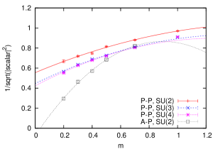
Figure 1: The mass-dependence of scalar eigenvalues at $L=0.707$ is plotted. The vertical axis represents $\left(\left\langle\sqrt{\frac{1}{NL^{2}}\int dx\int dy\,\mathop{Tr}\nolimits X_{i}^{2}}\right\rangle\right)^{-1}$, which is the inverse of the typical value of the scalar eigenvalues. In P-P boundary condition the scalar eigenvalues remain finite in the $m\to 0$ limit, while it diverges in A-P boundary condition. Fitting lines are quadratic polynomials of $m$.

A few remarks on the previous numerical simulations for $SU(2)$ gauge group [18, 19, 20, 21, 22] are in order here. In [18, 21, 22] the same regularization by introduction of the mass term is used. In these works the scalars seems to diverge in $m\to 0$ limit (it is the same as the one with A-P boundary condition, shown in Fig. 1. See also [39].) and hence it is plausible that the extrapolation to $m=0$ picks up the different phase from the bound state. It is plausible that this phase corresponds to the ${\mathbb{Z}}_{N}$-unbroken phase discussed in [26, 25]. On the other hand, the phase studied in [19, 20] should be the bound state, because in these papers the configurations have been made by using the bosonic part of the action and the effect of the fermionic part has been taken into account by the reweighting method. (Note that in the bosonic model the flat direction is lifted by quantum corrections and hence only bound states exist.)

3.2 Large-$N$ behavior of the Wilson loop and breakdown of ${\mathbb{Z}}_{N}$ symmetry

In this subsection, we study the Wilson loop $\mathop{Tr}\nolimits W_{\mu}/N$, where $W_{\mu}$ is a unitary matrix which is defined by

$$W_{x}(y)=P\exp\left(i\int_{0}^{L}dxA_{x}(x,y)\right),\qquad W_{y}(x)=P\exp\left(i\int_{0}^{L}dyA_{y}(x,y)\right).$$ (5)

On lattice, it can be obtained by multiplying the link variables. Because of the translational invariance of the model, the expectation value does not depend on the coordinate.

At finite $N$, there is a tunneling between different vacua related by a multiplication of a phase factor (3) and hence the expectation value $\langle\frac{1}{N}\mathop{Tr}\nolimits W_{\mu}\rangle$ is zero. (In the large-$N$ limit, the tunneling is suppressed and the expectation value can be non-zero.) Therefore, in order to see a possible symmetry breakdown at large-$N$, we fix the $({\mathbb{Z}}_{N})^{2}$ symmetry so that ${\rm Re}\sum_{j=1}^{k}\mathop{Tr}\nolimits W_{\mu}^{(j)}$ becomes maximum. That is, $W_{\mu}^{(j)}$ is replaced by $e^{2\pi in_{\mu}/N}W_{\mu}^{(j)}$ with a suitable $n_{\mu}$ which satisfies the above condition. In our numerical simulation, we have performed this ${\mathbb{Z}}_{N}$ fixing at each measurement.

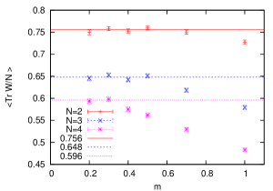
Figure 2: The expectation value of the Wilson loop $\langle\mathop{Tr}\nolimits W/N\rangle$ at $L=0.707$ is plotted for $0\leq m\leq 1$. At small values of $m$, the mass-dependence disappears.

Below we show the expectation values of the Wilson loops. We found that $\langle\frac{1}{N}\mathop{Tr}\nolimits W_{x}\rangle$ and $\langle\frac{1}{N}\mathop{Tr}\nolimits W_{y}\rangle$ are the same in the error. Therefore we use the average of them $\langle\frac{1}{N}\mathop{Tr}\nolimits W\rangle$, where $W\equiv(W_{x}+W_{y})/2$. (In the bosonic models, they take different values for some parameters [24, 32].)

In Fig. 2, the mass-dependence of the Wilson loop is plotted. (The size of the torus is $L=0.707$.) The mass-dependence disappears at small values of $m$, which allows us to use small fixed value of $m$. In practice, we use $m=0.2$, $0.3$ and $0.4$.

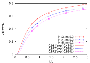
Figure 3: The expectation value of the Wilson loop $\langle\mathop{Tr}\nolimits W/N\rangle$ for $N=3,4$ and $5$. Mass parameter is $m=0.2$.

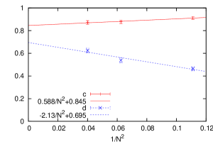
Figure 4: $N$-dependence of the coefficients in (6), $N=3,4$ and $5$. Mass parameter is $m=0.2$.

In Fig. 3, we plot the expectation value of the Wilson loop against the size of the torus $L$. For each $N$, the expectation value can be fitted by

$$\left\langle\frac{1}{N}\mathop{Tr}\nolimits W\right\rangle=c\times\exp\left(-d\cdot L\right),$$ (6)

where $c$ and $d$ are real and positive. By using the data at $L=0.471$, $0.707$, $1.061$, $1.414$ and $m=0.2$, we obtain $c=0.911\pm 0.012,d=0.464\pm 0.018$ for $N=3$, $c=0.877\pm 0.015,d=0.538\pm 0.022$ for $N=4$ and $c=0.872\pm 0.016,d=0.624\pm 0.020$ for $N=5$. Extrapolating these coefficients to $N=\infty$, we obtain $c=0.845\pm 0.009$ and $d=0.695\pm 0.040$ (Fig. 4). Therefore, in the large-$N$ limit, the expectation value of the Wilson loop is nonzero at finite volume, and hence the ${\mathbb{Z}}_{N}$ symmetry is broken. Note that the ${\mathbb{Z}}_{N}$ symmetry is restored in the large volume limit as expected.

3.3 Zero-volume limit

As we have seen above, the simulation data suggests that the ${\mathbb{Z}}_{N}$ symmetry is broken completely in the zero-volume limit, that is, the expectation value of the Wilson loop $\left\langle\frac{1}{N}\mathop{Tr}\nolimits W_{\mu}\right\rangle$ becomes close to $1$. Then the model reduces to the one-point reduction of 4d ${\cal N}=1$ SYM, which has been studied numerically in [29]. Hence, by comparing the 2d and 0d models, we can check the validity of our simulation.

Let us start with the action in two dimensions,

$$S_{2d}=N\int_{0}^{L}dx\int_{0}^{L}dy\,\mathop{Tr}\nolimits\left(\frac{1}{2}(D_{\mu}Y_{i})^{2}-\frac{1}{4}[Y_{i},Y_{j}]^{2}+\frac{1}{4}F_{\mu\nu}^{2}\right).$$ (7)

Here we denoted the scalar fields as $Y_{i}$ in order to distinguish them from the scalars $X_{I}$ in the zero-dimensional model. (For simplicity, we write down only the bosonic part.) By neglecting nonzero-modes, this action reduces to the zero-dimensional one. By using $X_{I}=(X_{\mu},X_{i})$ defined by

$$X_{i}=L^{-3/2}\int_{0}^{L}dx\int_{0}^{L}dy\,Y_{i},\quad X_{\mu}=L^{-3/2}\int_{0}^{L}dx\int_{0}^{L}dy\,A_{\mu},$$ (8)

we obtain the zero-dimensional model with the canonical normalization,

$$S_{0d}=-\frac{N}{4}\mathop{Tr}\nolimits[X_{I},X_{J}]^{2}.$$ (9)

Here, the gauge field $A_{\mu}$ can be obtained by

$$\frac{1}{2}\left[-i(W_{\mu}-1)+c.c.\right]\simeq\int_{0}^{L}dx^{\mu}A_{\mu},$$ (10)

where in the r.h.s. the index $\mu$ is not contracted. When we consider the $k\times k$ square lattice, we can calculate $k$ Wilson loops along both $x$ and $y$ directions, $W_{\mu}^{(1)},\cdots,W_{\mu}^{(k)}$. $X_{\mu}$ can be obtained as

$$X_{\mu}\simeq\frac{1}{k\sqrt{L}}\sum_{j=1}^{k}\frac{1}{2}\left[-i(W_{\mu}^{(j)}-1)+h.c.\right].$$ (11)

There is a subtlety in the discussion above – “zero-mode” is not a gauge-invariant notion. (A constant field configuration, which corresponds to the zero-dimensional model, can be transformed to rapidly varying configuration just by a gauge transformation!) Therefore, we have to choose a suitable gauge in which zero modes reproduce the zero-dimensional matrix model [40]. In the current setup, we should maximize (resp. minimize) the zero-mode (resp. nonzero-mode) contributions, so that the configuration is as static as possible. For that purpose we choose the gauge so that $\mathop{Tr}\nolimits(X_{i}^{2}+X_{\mu}^{2})$ is maximum.

In this gauge we can compare the small volume behavior with zero-dimensional matrix model. The simplest quantity is $\left\langle-\frac{1}{N}\mathop{Tr}\nolimits[X_{I},X_{J}]^{2}\right\rangle$, which can be evaluated exactly [41]:

$$\left\langle-\frac{1}{N}\mathop{Tr}\nolimits[X_{1},X_{2}]^{2}\right\rangle=\left\langle-\frac{1}{N}\mathop{Tr}\nolimits[X_{3},X_{4}]^{2}\right\rangle=\frac{1}{2}\left(1-\frac{1}{N^{2}}\right).$$ (12)

In Fig. 6 and Fig. 6, the corresponding quantity in two-dimensional SYM is plotted. In Fig. 8 and Fig. 8, $\left\langle\sqrt{\sum_{\mu=1}^{2}\frac{1}{N}\mathop{Tr}\nolimits X_{\mu}^{2}}\right\rangle$ and the corresponding quantity in two dimensions are plotted. In these plots, the results at $m=0$ is obtained by extrapolating results at $m=0.2,0.3$ and $m=0.4$ by a straight line. Then we have fitted them by a polynomial $A+BL+CL^{2}$. We have evaluated $\left\langle\sqrt{\sum_{\mu=1}^{2}\frac{1}{N}\mathop{Tr}\nolimits X_{\mu}^{2}}\right\rangle$ numerically in 0d theory and found that it is $1.78\pm 0.03$ for $SU(3)$. In Fig. 6, Fig. 6 and Fig. 8 the data is consistent with 0d model results for $SU(3)$. (In Fig. 8, the extrapolated value differs slightly from the 0d result. One possible reason is this quantity is sensitive to the error in the approximation in (11), which is exact in the limit $W_{\mu}=\textbf{1}_{N}$.) Since our 2d simulation is smoothly connected to the 0d model, we conclude that the bound state we have constructed is exactly the one discussed in §2.2.

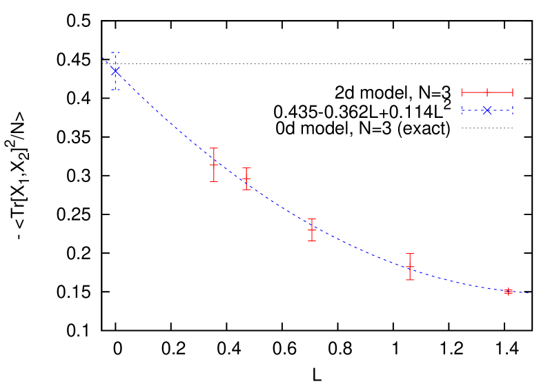
Figure 5: $\left\langle-\frac{1}{N}\mathop{Tr}\nolimits[X_{1},X_{2}]^{2}\right\rangle$, $N=3$, calculated from gauge fields.

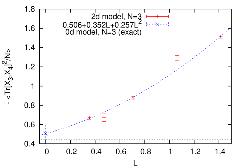
Figure 6: $\left\langle-\frac{1}{N}\mathop{Tr}\nolimits[X_{3},X_{4}]^{2}\right\rangle$, $N=3$, calculated from scalar fields.

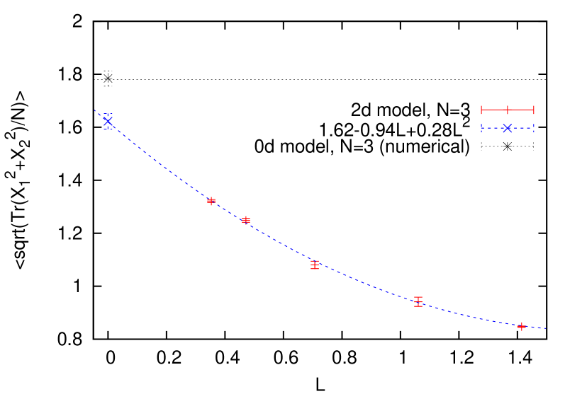
Figure 7: $\left\langle\sqrt{\frac{1}{N}\mathop{Tr}\nolimits\left(X_{1}^{2}+X_{2}^{2}\right)}\right\rangle$, $N=3$, calculated from gauge fields.

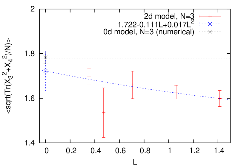
Figure 8: $\left\langle\sqrt{\frac{1}{N}\mathop{Tr}\nolimits\left(X_{3}^{2}+X_{4}^{2}\right)}\right\rangle$, $N=3$, calculated from scalar fields.

3.4 Supersymmetry

It is important to study whether the bound state preserves supersymmetry or not. Here we show the expectation value of the action. In the Sugino model the action is of the form

$$S=\{Q,{\cal O}\},$$ (13)

where $Q$ is one of four supercharges which is exactly kept in the regularization. Therefore, the expectation value of the action must be zero if the vacuum is invariant under the supersymmetry generated by $Q$. As we can see from Fig. 9, the expectation value of the action is consistent with zero.

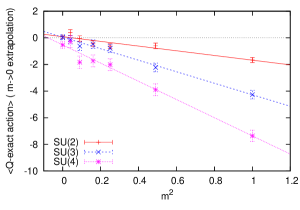
Figure 9: Mass-dependence of the action at $L=0.707$. The points at $m=0$ are obtained by extrapolations. In the $m\to 0$ limit, where the continuum theory becomes supersymmetric, the expectation value is consistent with zero ( SU(4) case seems nonzero but consistent with zero in 2 standard deviations).

Strictly speaking, there is a subtlety for studying the breakdown of the supersymmetry with periodic boundary conditions. The reason is as follows [20]. In the simulation, we obtain the expectation values normalized as

$$\frac{\langle 0|\{Q,{\cal O}\}|0\rangle}{\langle 0|0\rangle}$$ (14)

where the denominator $\langle 0|0\rangle$ is the partition function. In order for the simulation to make sense, the denominator must be nonzero, but this condition can be broken. Indeed, if the continuum spectrum is absent and the Witten index is well-defined, then the partition function with the periodic boundary conditions is nothing but the Witten index, which is zero if the supersymmetry is spontaneously broken. In the present case, because the continuum spectrum exists due to the existence of the unbounded state and there is an ambiguity for the definition of the Witten index, the above argument cannot be applied straightforwardly. Although it is difficult to exclude the possibility that the partition function is zero, we believe the partition function is nonzero because this system does not suffer from the sign problem. Clarification of this point is desirable.

In order to see whether the supersymmetry is spontaneously broken or not, the simplest and unambiguous way is to put the theory at finite temperature and calculate the energy density [20]. Supersymmetry is not broken if and only if the energy density is zero at zero temperature. It is an important future problem to study 2d theory at large-$N$ and at finite temperature, and confirm that the energy converges to zero.

As we will see in § 3.5, it is plausible that the explicit supersymmetry breaking lattice artifacts disappears in the continuum limit. Then, the fact that the expectation value of the action is zero suggests the absence of the spontaneous supersymmetry breaking. It is desirable to check it more rigorously by measuring the energy of the system.

3.5 Convergence to the continuum limit

In this subsection, we show that the lattice spacing used in the current simulation is small enough to study the system quantitatively.

gauge group	volume	lattice size
$SU(2)$	0.707	$4\times 4$
$SU(2)$	1.414	$8\times 8,\ 6\times 6,\ 5\times 5,\ 4\times 4$
$SU(3)$	0.354, 0.471, 0.707	$4\times 4$
$SU(3)$	1.061, 1.414	$6\times 6$
$SU(4)$	0.354, 0.471, 0.707	$4\times 4$
$SU(4)$	1.061, 1.414	$6\times 6$
$SU(5)$	0.354, 0.471, 0.707, 1.061, 1.414	$4\times 4$

Table 2: A list of lattice sizes used in this work.

The lattice sizes used in this work are listed in Table. 2. In Fig. 10, Fig. 11 and Fig. 12, we plot the lattice spacing dependences of the extent of the scalar eigenvalues, the Wilson loop and the action. Lattice size was taken to be $4\times 4$, $5\times 5$, $6\times 6$ and $8\times 8$ and other parameters are taken to be $N=2,L=1.414,m=0.2$. It turns out that the expectation values, especially that of the Wilson loop, are not sensitive to the lattice spacing used in the simulation. Note that $4\times 4$ lattice at $L=1.414$ is the coarsest one in this work. Therefore the numerical data used in the previous sections is sufficiently close to the continuum limit.

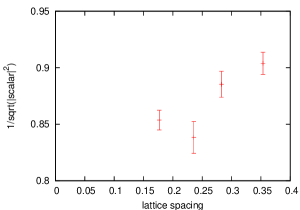
Figure 10: Dependence of the inverse of the scalar norm $\left(\left\langle\sqrt{\frac{1}{NL^{2}}\int dx\int dy\,\mathop{Tr}\nolimits X_{i}^{2}}\right\rangle\right)^{-1}$ on the lattice spacing at $N=2,L=1.414,m=0.2$.

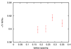
Figure 11: Dependence of the Wilson loop to the lattice spacing at $N=2,L=1.414,m=0.2$.

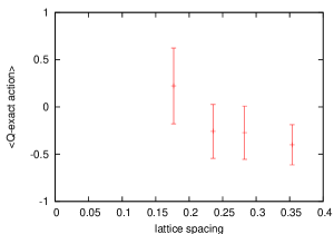
Figure 12: Dependence of the action on the lattice spacing at $N=2,L=1.414,m=0.2$.

In order to see that the supersymmetries which are broken by a lattice artifact are restored in the continuum limit, we utilize the discrete symmetry of the system which is related to the R-symmetry. The action in the continuum has the following discrete symmetries (we follow the notation in the Appendix):

$$\frac{\eta}{2} \to\chi, \chi \to-\frac{\eta}{2}, \psi_{0} \to\psi_{1}, \psi_{1} \to-\psi_{0}$$ (15)

and

$$\frac{\eta}{2} \to\psi_{1}, \chi \to\psi_{0}, \psi_{1} \to\frac{\eta}{2}, \psi_{0} \to\chi, \phi \to-\bar{\phi}, \bar{\phi} \to-\phi.$$ (16)

Because of these symmetries, in the continuum limit, all four Yukawa interaction terms $\mathcal{L}_{F1},...,\mathcal{L}_{F4}$ (for explicit forms, see Appendix) should give an identical expectation value. In Fig. 13, we plot them for the coarsest ($L=1.414$ with $4\times 4$ lattice) and the finest ($L=0.354$ with $4\times 4$ lattice) cases with $N=5$. We also plot $N=2$ case using the same configuration used to plot Fig. 8 in [18]. The plots show that the expectation values from the finest lattice are almost degenerated for all $\mathcal{L}_{Fi}$ ($i=1,...4$) and it strongly suggests that this discrete symmetry is restored in the continuum limit. Therefore we can expect that supersymmetries broken by a lattice artifact are restored in the continuum limit, because they are related to the exactly kept supersymmetry via this discrete symmetry. Note that, although the coarsest case would have some effects from the lattice artifacts, at least for the quantities like the Wilson loop such effects are negligible, as we have seen above.

A remark on the previous simulation [18] is in order here. In [18], the restoration of supersymmetries which are explicitly broken by lattice artifacts has been studied. In that work, expectation values of two-point functions are used. (In the present simulation, this technique cannot be used because the lattice is too small to calculate the two-point functions.) In Fig. 8 and 9 in [18], four different two-point functions are plotted for P-P case which should be degenerated because of the above discrete symmetries. The plots, however, does not show the degenerate behavior and hence it seems that the simulation is far from the continuum limit. The non-degenerate behavior is again found in the lowest plot in Fig. 13 while in the first plot from the current simulation almost degenerated behavior can be seen.

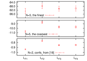
Figure 13: Expectation values of $\mathcal{L}_{Fi}(i=1,...,4)$, the almost degenerate behavior implies the that the simulation is close to the continuum limit. The lowest plot uses the same configuration used to plot Fig. 8 in [18].

4 Conclusion and discussions

In this paper we have studied large-$N$ properties of two-dimensional ${\cal N}=(2,2)$ SYM. Especially we have established the existence of the bound state in which scalar eigenvalues clump around the origin. It makes the simulation well-defined in spite of the existence of the flat direction along which scalar eigenvalues spread to infinity. We also have shown numerically that at finite volume global $(\mathbb{Z}_{N})^{2}$ is broken. This symmetry is restored in the large volume limit.

If the $({\mathbb{Z}}_{N})^{2}$ symmetry were not broken, then because of the Eguchi-Kawai equivalence the expectation values of the loops would not depend on the volume in the large-$N$ limit [33, 24]. The Eguchi-Kawai equivalence works for bosonic Yang-Mills only above a critical volume [24] because the $({\mathbb{Z}}_{N})^{4}$ symmetry is broken below it. The twisted [43] and quenched [44] Eguchi-Kawai models were believed to cure this problem, but recently turned out to fail in the large-$N$ limit [45, 46]. The reason is that the backgrounds collapses due to large fluctuations. (Another deformation has been proposed in [47].) For supersymmetric theories the ${\mathbb{Z}}_{N}$ symmetry was expected not to be broken, but as shown in this paper, it is not necessarily the case. However, once we combine the idea of twisted or quenched Eguchi-Kawai model with the supersymmetry then the ${\mathbb{Z}}_{N}$-unbroken background becomes stable [48] and the Eguchi-Kawai equivalence can hold. A concrete proposal has been given in [36] . Studying this direction further is very important, because using the Eguchi-Kawai equivalence we can regularize planar SYM in higher dimensions (3d and 4d) without using lattice, and hence we may avoid the difficulties in lattice SUSY.

Although finite-temperature properties of the bound state is very interesting in connection to the black hole thermodynamics, it is much more difficult to study because we need to take $N$ to be rather large. The same difficulty exists in matrix quantum mechanics, though large enough $N$ (say $N=16$) can be taken in that case [9] because the model requires less computational resources. In [11], to avoid this difficulty at rather small $N$, finite-temperature properties of the matrix quantum mechanics have been studied by performing the simulation with the periodic boundary condition and then taking into account the effect of the antiperiodic boundary condition by the reweighting method. This method would work for the ${\mathbb{Z}}_{N}$-broken phase (“black hole” and “non-uniform black string”). However, for the ${\mathbb{Z}}_{N}$-unbroken phase, this method might not work because we expect a severer overlapping problem. In any case, we expect an unambiguous study of the thermal properties with large enough $N$ will be possible in near future. It will provide us with valuable insights into black hole/black string physics.

Acknowledgment

A part of the program used in this work was developed from the ones used in collaborations of I. K. with H. Suzuki. The authors would like to thank O. Aharony, B. Bringoltz, D. Kadoh, S. Matsuura, J. Nishimura, T. Nishioka, D. Robles-Llana, H. Shimada, H. Suzuki, M. Ünsal and L. Yaffe for discussions. The computations were carried out on PC clusters at Yukawa Institute and RIKEN RSCC. The work of I. K. was supported by the Nishina Memorial Foundation.

Appendix A Simulation details

A.1 The Sugino model

We consider the ${\cal N}=(2,2)$ supersymmetric Yang-Mills theory on $T^{2}$, whose action is given by

$$S_{continuum}$$

$$=N\int_{0}^{L_{x}}dx\int_{0}^{L_{y}}dy\,\mathop{Tr}\nolimits\left\{\frac{1}{4}F_{\mu\nu}^{2}+\frac{1}{2}(D_{\mu}X_{i})^{2}-\frac{1}{4}[X_{i},X_{j}]^{2}-\frac{i}{2}\bar{\psi}\Gamma^{\mu}D_{\mu}\psi-\frac{1}{2}\bar{\psi}\Gamma^{i}[X_{i},\psi]\right\},$$ (17)

which is obtained from four-dimensional ${\cal N}=1$ SYM through the dimensional reduction.

As a discretization, we use Sugino’s lattice action [16] ,

$$S_{lattice}=a_{x}a_{y}\sum_{\vec{x}}\left\{\sum_{i=1}^{3}{\cal L}_{Bi}(\vec{x})+\sum_{i=1}^{6}{\cal L}_{Fi}(\vec{x})\right\}+{\rm(auxiliary\ field)},$$ (18)

where

$${\cal L}_{B1}(\vec{x}) =\frac{N}{4a_{x}^{2}a_{y}^{2}}\mathop{Tr}\nolimits[\phi(\vec{x}),\bar{\phi}(\vec{x})]^{2},$$ (19)

$${\cal L}_{B2}(\vec{x}) =\frac{N}{4a_{x}^{2}a_{y}^{2}}\mathop{Tr}\nolimits\hat{\Phi}_{TL}(\vec{x})^{2},$$ (20)

$${\cal L}_{B3}(\vec{x}) =\frac{N}{a_{x}^{3}a_{y}}\mathop{Tr}\nolimits\bigl{\{}\left(\phi(\vec{x})-U_{x}(\vec{x})\phi(\vec{x}+a_{x}\hat{x})U_{x}(\vec{x})^{-1}\right)$$

$$\hskip 85.35826pt\times\left(\bar{\phi}(\vec{x})-U_{x}(\vec{x})\bar{\phi}(\vec{x}+a_{x}\hat{x})U_{x}(\vec{x})^{-1}\right)\bigl{\}}$$

$$+\frac{N}{a_{x}a_{y}^{3}}\mathop{Tr}\nolimits\bigl{\{}\left(\phi(\vec{x})-U_{y}(\vec{x})\phi(\vec{x}+a_{y}\hat{y})U_{y}(\vec{x})^{-1}\right)$$

$$\hskip 85.35826pt\times\left(\bar{\phi}(\vec{x})-U_{y}(\vec{x})\bar{\phi}(\vec{x}+a_{y}\hat{y})U_{y}(\vec{x})^{-1}\right)\bigl{\}}$$ (21)

and

$${\cal L}_{F1}(\vec{x}) =-\frac{N}{4a_{x}^{2}a_{y}^{2}}\mathop{Tr}\nolimits\left(\eta(\vec{x})[\phi(\vec{x}),\eta(\vec{x})]\right),$$ (22)

$${\cal L}_{F2}(\vec{x}) =-\frac{N}{a_{x}^{2}a_{y}^{2}}\mathop{Tr}\nolimits\left(\chi(\vec{x})[\phi(\vec{x}),\chi(\vec{x})]\right),$$ (23)

$${\cal L}_{F3}(\vec{x}) =-\frac{N}{a_{x}^{3}a_{y}}\mathop{Tr}\nolimits\left\{\psi_{0}(\vec{x})\psi_{0}(\vec{x})\left(\bar{\phi}(\vec{x})+U_{x}(\vec{x})\bar{\phi}(\vec{x}+a_{x}\hat{x})U_{x}(\vec{x})^{-1}\right)\right\},$$ (24)

$${\cal L}_{F4}(\vec{x}) =-\frac{N}{a_{x}a_{y}^{3}}\mathop{Tr}\nolimits\left\{\psi_{1}(\vec{x})\psi_{1}(\vec{x})\left(\bar{\phi}(\vec{x})+U_{y}(\vec{x})\bar{\phi}(\vec{x}+a_{y}\hat{y})U_{y}(\vec{x})^{-1}\right)\right\},$$ (25)

$${\cal L}_{F5}(\vec{x}) =i\frac{N}{a_{x}^{2}a_{y}^{2}}\mathop{Tr}\nolimits\left(\chi(\vec{x})\cdot Q\hat{\Phi}(\vec{x})\right),$$ (26)

$${\cal L}_{F6}(\vec{x}) =-i\frac{N}{a_{x}^{3}a_{y}}\mathop{Tr}\nolimits\bigl{\{}\psi_{0}\left(\eta(\vec{x})-U_{x}(\vec{x})\eta(\vec{x}+a_{x}\hat{x})U_{x}(\vec{x})^{-1}\right)\bigl{\}}$$

$$-i\frac{N}{a_{x}a_{y}^{3}}\mathop{Tr}\nolimits\bigl{\{}\psi_{1}\left(\eta(\vec{x})-U_{y}(\vec{x})\eta(\vec{x}+a_{y}\hat{y})U_{y}(\vec{x})^{-1}\right)\bigl{\}},$$ (27)

where $U(\vec{x},\mu)$ are gauge link variables, $\phi(\vec{x})$ is a complex scalar, $\eta(\vec{x})$, $\chi(\vec{x})$ and $\psi_{\mu}(\vec{x})$ are fermion field, $a_{x}$ and $a_{y}$ are lattice spacings , $\epsilon$ is a real parameter which must be chosen appropriately for each $N$ (in this work, we used $\epsilon=2.6$),

$$\hat{\Phi}(\vec{x}) =\frac{-i(P(\vec{x})-P(\vec{x})^{-1})}{1-|1-P(\vec{x})|^{2}/\epsilon^{2}},\qquad\hat{\Phi}_{TL}(\vec{x})=\hat{\Phi}(\vec{x})-\frac{1}{N}\left(\mathop{Tr}\nolimits\hat{\Phi}(\vec{x})\right)\cdot\textbf{1},$$ (28)

where $P(\vec{x})=U_{x}(\vec{x})U_{y}(\vec{x}+\hat{x})U_{x}^{\dagger}(\vec{x}+\hat{y})U_{y}^{\dagger}(\vec{x})$ is the plaquette variable, and $Q$ generates one of the four supersymmetries,

$$QU_{\mu}(\vec{x}) =i\psi_{\mu}(\vec{x})U_{\mu}(\vec{x}),$$ (29)

$$Q\psi_{\mu}(\vec{x}) =i\psi_{\mu}(\vec{x})\psi_{\mu}(\vec{x})-i\bigl{(}\phi(\vec{x})-U_{\mu}(\vec{x})\phi(\vec{x}+a_{\mu}\hat{\mu})U_{\mu}(\vec{x})^{-1}\bigr{)},$$ (30)

$$Q\phi(\vec{x}) =0,$$ (31)

$$Q\chi(\vec{x}) =H(\vec{x}),$$ (32)

$$QH(\vec{\vec{x}}) =[\phi(\vec{x}),\chi(\vec{x})],$$ (33)

$$Q\bar{\phi}(\vec{x}) =\eta(\vec{x}),$$ (34)

$$Q\eta(\vec{x}) =[\phi(\vec{x}),\bar{\phi}(\vec{x})].$$ (35)

Sugino’s action $S_{lattice}$ is invariant under the supersymmetry generated by $Q$, because $Q$ is nilpotent up to gauge transformation and $S$ can be written in a $Q$-exact form.

In [16], using super-renormalizability and symmetry argument, it was shown that other three supersymmetries, which is broken by a lattice artifact at the discretized level, is restored in the continuum limit. Furthermore, in [18], this restoration has been confirmed explicitly by the Monte-Carlo simulation.

A.2 Simulation

We have adopted the rational hybrid Monte-Carlo algorithm [50]. We have use the code [51] based on the Remez algorithm to find necessary coefficients in the simulation. In 2d ${\cal N}=(2,2)$ SYM, the complex phase of the fermion determinant is absent in the continuum limit and at discretized level only small phase appears as a lattice artifact. In this work we have ignored it. Fermi QCD/MDP [52] has been used to develop the simulation code.

Because of the limitation of the resources, we have concentrated on the square torus, $L_{x}=L_{y}=L$. We took the number of sites and lattice spacings in two directions to be the same. For each set of parameters, we have collected 1000 $-$ 2000 samples of configurations. We have evaluated the error by using the Jack Knife method and it turned out the autocorrelations are sufficiently small.

References

- [1] T. Banks, W. Fischler, S. H. Shenker and L. Susskind, “M theory as a matrix model: A conjecture,” Phys. Rev. D 55, 5112 (1997) [arXiv:hep-th/9610043].
- [2] N. Ishibashi, H. Kawai, Y. Kitazawa and A. Tsuchiya, “A large-N reduced model as superstring,” Nucl. Phys. B 498, 467 (1997) [arXiv:hep-th/9612115].
- [3] L. Motl, “Proposals on nonperturbative superstring interactions,” arXiv:hep-th/9701025. R. Dijkgraaf, E. P. Verlinde and H. L. Verlinde, “Matrix string theory,” Nucl. Phys. B 500, 43 (1997) [arXiv:hep-th/9703030].
- [4] J. M. Maldacena, “The large N limit of superconformal field theories and supergravity,” Adv. Theor. Math. Phys. 2, 231 (1998) [Int. J. Theor. Phys. 38, 1113 (1999)] [arXiv:hep-th/9711200].
- [5] N. Itzhaki, J. M. Maldacena, J. Sonnenschein and S. Yankielowicz, “Supergravity and the large N limit of theories with sixteen supercharges,” Phys. Rev. D 58, 046004 (1998) [arXiv:hep-th/9802042].
- [6] J. Giedt, “Advances and applications of lattice supersymmetry,” PoS LAT2006, 008 (2006) [arXiv:hep-lat/0701006].
- [7] S. Catterall, D. B. Kaplan and M. Unsal, “Exact lattice supersymmetry,” arXiv:0903.4881 [hep-lat].
- [8] M. Hanada, J. Nishimura and S. Takeuchi, “Non-lattice simulation for supersymmetric gauge theories in one dimension,” Phys. Rev. Lett. 99, 161602 (2007) [arXiv:0706.1647 [hep-lat]].
- [9] K. N. Anagnostopoulos, M. Hanada, J. Nishimura and S. Takeuchi, “Monte Carlo studies of supersymmetric matrix quantum mechanics with sixteen supercharges at finite temperature,” Phys. Rev. Lett. 100, 021601 (2008) [arXiv:0707.4454 [hep-th]].
- [10] S. Catterall and T. Wiseman, “Towards lattice simulation of the gauge theory duals to black holes and hot strings,” JHEP 0712, 104 (2007) [arXiv:0706.3518 [hep-lat]].
- [11] S. Catterall and T. Wiseman, “Black hole thermodynamics from simulations of lattice Yang-Mills theory,” Phys. Rev. D 78, 041502 (2008) [arXiv:0803.4273 [hep-th]].
- [12] M. Hanada, A. Miwa, J. Nishimura and S. Takeuchi, “Schwarzschild radius from Monte Carlo calculation of the Wilson loop in supersymmetric matrix quantum mechanics,” Phys. Rev. Lett. 102, 181602 (2009) [arXiv:0811.2081 [hep-th]]. M. Hanada, Y. Hyakutake, J. Nishimura and S. Takeuchi, “Higher derivative corrections to black hole thermodynamics from supersymmetric matrix quantum mechanics,” Phys. Rev. Lett. 102, 191602 (2009) [arXiv:0811.3102 [hep-th]].
- [13] R. Gregory and R. Laflamme, “Black strings and p-branes are unstable,” Phys. Rev. Lett. 70, 2837 (1993) [arXiv:hep-th/9301052].
- [14] L. Susskind, “Matrix theory black holes and the Gross Witten transition,” hep-th/9805115. J. L. F. Barbon, I. I. Kogan and E. Rabinovici, “On stringy thresholds in SYM/AdS thermodynamics,” Nucl. Phys. B 544, 104 (1999) [arXiv:hep-th/9809033]. M. Li, E. J. Martinec and V. Sahakian, “Black holes and the SYM phase diagram,” Phys. Rev. D 59, 044035 (1999) [arXiv:hep-th/9809061]. E. J. Martinec and V. Sahakian, “Black holes and the SYM phase diagram. II,” Phys. Rev. D 59, 124005 (1999) [arXiv:hep-th/9810224]. O. Aharony, J. Marsano, S. Minwalla and T. Wiseman, “Black hole - black string phase transitions in thermal 1+1 dimensional supersymmetric Yang-Mills theory on a circle,” Class. Quant. Grav. 21, 5169 (2004) [arXiv:hep-th/0406210]. T. Harmark and N. A. Obers, “New phases of near-extremal branes on a circle,” JHEP 0409, 022 (2004) [arXiv:hep-th/0407094].
- [15] O. Aharony, J. Marsano, S. Minwalla, K. Papadodimas, M. Van Raamsdonk and T. Wiseman, “The phase structure of low dimensional large N gauge theories on tori,” JHEP 0601, 140 (2006) [arXiv:hep-th/0508077].
- [16] F. Sugino, “Super Yang-Mills theories on the two-dimensional lattice with exact supersymmetry,” JHEP 0403, 067 (2004) [arXiv:hep-lat/0401017].
- [17] A. G. Cohen, D. B. Kaplan, E. Katz and M. Unsal, “Supersymmetry on a Euclidean spacetime lattice. I: A target theory with four supercharges,” JHEP 0308, 024 (2003) [arXiv:hep-lat/0302017]. A. D’Adda, I. Kanamori, N. Kawamoto and K. Nagata, “Exact extended supersymmetry on a lattice: Twisted N = 2 super Yang-Mills in two dimensions,” Phys. Lett. B 633, 645 (2006) [arXiv:hep-lat/0507029]. S. Catterall, “A geometrical approach to N = 2 super Yang-Mills theory on the two dimensional lattice,” JHEP 0411, 006 (2004) [arXiv:hep-lat/0410052]. H. Suzuki and Y. Taniguchi, “Two-dimensional N = (2,2) super Yang-Mills theory on the lattice via dimensional reduction,” JHEP 0510, 082 (2005) [arXiv:hep-lat/0507019].
- [18] I. Kanamori and H. Suzuki, “Restoration of supersymmetry on the lattice: Two-dimensional supersymmetric Yang-Mills theory,” Nucl. Phys. B 811, 420 (2009) [arXiv:0809.2856 [hep-lat]].
- [19] H. Suzuki, “Two-dimensional super Yang-Mills theory on computer,” JHEP 0709, 052 (2007) [arXiv:0706.1392 [hep-lat]].
- [20] I. Kanamori, H. Suzuki and F. Sugino, “Euclidean lattice simulation for the dynamical supersymmetry breaking,” Phys. Rev. D 77, 091502 (2008) [arXiv:0711.2099 [hep-lat]]. I. Kanamori, F. Sugino and H. Suzuki, “Observing dynamical supersymmetry breaking with euclidean lattice simulations,” Prog. Theor. Phys. 119, 797 (2008) [arXiv:0711.2132 [hep-lat]].
- [21] I. Kanamori and H. Suzuki, “Some physics of the two-dimensional supersymmetric Yang-Mills theory: Lattice Monte Carlo study,” Phys. Lett. B 672, 307 (2009) [arXiv:0811.2851 [hep-lat]].
- [22] I. Kanamori, “Vacuum energy of two-dimensional N=(2,2) super Yang-Mills theory,” Phys. Rev. D 79, 115015 (2009) [arXiv:0902.2876 [hep-lat]].
- [23] S. Catterall, “First results from simulations of supersymmetric lattices,” JHEP 0901, 040 (2009) [arXiv:0811.1203 [hep-lat]].
- [24] R. Narayanan and H. Neuberger, “Large N reduction in continuum,” Phys. Rev. Lett. 91, 081601 (2003) [arXiv:hep-lat/0303023].
- [25] M. Hanada, S. Matsuura, J. Nishimura and D. Robles-Llana, in preparation.
- [26] P. Kovtun, M. Unsal and L. G. Yaffe, “Volume independence in large N(c) QCD-like gauge theories,” JHEP 0706, 019 (2007) [arXiv:hep-th/0702021].
- [27] N. M. Davies, T. J. Hollowood, V. V. Khoze and M. P. Mattis, “Gluino condensate and magnetic monopoles in supersymmetric gluodynamics,” Nucl. Phys. B 559, 123 (1999) [arXiv:hep-th/9905015].
- [28] W. Krauth and M. Staudacher, “Eigenvalue distributions in Yang-Mills integrals,” Phys. Lett. B 453, 253 (1999) [arXiv:hep-th/9902113].
- [29] J. Ambjorn, K. N. Anagnostopoulos, W. Bietenholz, T. Hotta and J. Nishimura, “Large N dynamics of dimensionally reduced 4D SU(N) super Yang-Mills theory,” JHEP 0007, 013 (2000) [arXiv:hep-th/0003208].
- [30] P. Austing and J. F. Wheater, “Convergent Yang-Mills matrix theories,” JHEP 0104, 019 (2001) [arXiv:hep-th/0103159].
- [31] N. Kawahara, J. Nishimura and S. Takeuchi, “Phase structure of matrix quantum mechanics at finite temperature,” JHEP 0710, 097 (2007) [arXiv:0706.3517 [hep-th]].
- [32] M. Hanada and T. Nishioka, “Cascade of Gregory-Laflamme Transitions and U(1) Breakdown in Super Yang-Mills,” JHEP 0709, 012 (2007) [arXiv:0706.0188 [hep-th]].
- [33] T. Eguchi and H. Kawai, “Reduction Of Dynamical Degrees Of Freedom In The Large N Gauge Theory,” Phys. Rev. Lett. 48, 1063 (1982).
- [34] B. Bringoltz, “Large-N volume reduction of lattice QCD with adjoint Wilson fermions at weak-coupling,” JHEP 0906, 091 (2009) [arXiv:0905.2406 [hep-lat]].
- [35] P. F. Bedaque, M. I. Buchoff, A. Cherman and R. P. Springer, “Can fermions save large N dimensional reduction?,” arXiv:0904.0277 [hep-th].
- [36] T. Ishii, G. Ishiki, S. Shimasaki and A. Tsuchiya, “N=4 Super Yang-Mills from the Plane Wave Matrix Model,” Phys. Rev. D 78, 106001 (2008) [arXiv:0807.2352 [hep-th]].
- [37] M. Hanada, L. Mannelli and Y. Matsuo, “Four-dimensional N=1 super Yang-Mills from matrix model,” arXiv:0905.2995 [hep-th]. M. Hanada, L. Mannelli and Y. Matsuo, “Large- reduced models of supersymmetric quiver and Chern-Simons gauge theories,” in preparation.
- [38] H. Aoki, S. Iso, H. Kawai, Y. Kitazawa and T. Tada, “Space-time structures from IIB matrix model,” Prog. Theor. Phys. 99, 713 (1998) [arXiv:hep-th/9802085].
- [39] I. Kanamori, “RHMC simulation of two-dimensional N=(2,2) super Yang-Mills with exact supersymmetry,” PoS LATTICE 2008, 232 (2008) [arXiv:0809.0655 [hep-lat]].
- [40] T. Azeyanagi, M. Hanada, T. Hirata and H. Shimada, “On the shape of a D-brane bound state and its topology change,” JHEP 0903, 121 (2009) [arXiv:0901.4073 [hep-th]].
- [41] T. Hotta, J. Nishimura and A. Tsuchiya, “Dynamical aspects of large N reduced models,” Nucl. Phys. B 545, 543 (1999) [arXiv:hep-th/9811220].
- [42] A. V. Smilga, “Comments on thermodynamics of supersymmetric matrix models,” Nucl. Phys. B 818, 101 (2009) [arXiv:0812.4753 [hep-th]].
- [43] A. Gonzalez-Arroyo and M. Okawa, “The Twisted Eguchi-Kawai Model: A Reduced Model For Large N Lattice Gauge Theory,” Phys. Rev. D 27, 2397 (1983).
- [44] G. Bhanot, U. M. Heller and H. Neuberger, “The Quenched Eguchi-Kawai Model,” Phys. Lett. B 113, 47 (1982). G. Parisi, “A Simple Expression For Planar Field Theories,” Phys. Lett. B 112, 463 (1982). D. J. Gross and Y. Kitazawa, “A Quenched Momentum Prescription For Large N Theories,” Nucl. Phys. B 206, 440 (1982).
- [45] T. Azeyanagi, M. Hanada, T. Hirata and T. Ishikawa, “Phase structure of twisted Eguchi-Kawai model,” JHEP 0801, 025 (2008) [arXiv:0711.1925 [hep-lat]]. M. Teper and H. Vairinhos, “Symmetry breaking In twisted Eguchi-Kawai models,” Phys. Lett. B 652, 359 (2007) [arXiv:hep-th/0612097]. W. Bietenholz, J. Nishimura, Y. Susaki and J. Volkholz, “A non-perturbative study of 4d U(1) non-commutative gauge theory: The fate of one-loop instability,” JHEP 0610, 042 (2006) [arXiv:hep-th/0608072].
- [46] B. Bringoltz and S. R. Sharpe, “Breakdown of large-N quenched reduction in SU(N) lattice gauge theories,” Phys. Rev. D 78, 034507 (2008) [arXiv:0805.2146 [hep-lat]].
- [47] M. Unsal and L. G. Yaffe, “Center-stabilized Yang-Mills theory: confinement and large volume independence,” Phys. Rev. D 78, 065035 (2008) [arXiv:0803.0344 [hep-th]].
- [48] T. Azeyanagi, M. Hanada and T. Hirata, “On Matrix Model Formulations of Noncommutative Yang-Mills Theories,” Phys. Rev. D 78, 105017 (2008) [arXiv:0806.3252 [hep-th]].
- [49] G. Ishiki, S. W. Kim, J. Nishimura and A. Tsuchiya, “Deconfinement phase transition in super Yang-Mills theory on from supersymmetric matrix quantum mechanics,” Phys. Rev. Lett. 102, 111601 (2009) [arXiv:0810.2884 [hep-th]]. G. Ishiki, S. W. Kim, J. Nishimura and A. Tsuchiya, “Testing a novel large-N reduction for N=4 super Yang-Mills theory on ,” arXiv:0907.1488 [hep-th]. Y. Kitazawa and K. Matsumoto, “ Supersymmetric Yang-Mills on in Plane Wave Matrix Model at Finite Temperature,” arXiv:0811.0529 [hep-th].
- [50] M. A. Clark, A. D. Kennedy and Z. Sroczynski, “Exact 2+1 flavour RHMC simulations,” Nucl. Phys. Proc. Suppl. 140, 835 (2005) [arXiv:hep-lat/0409133].
- [51] M. A. Clark and A. D. Kennedy, http://www.ph.ed.ac.uk/ mike/remez, 2005.
- [52] M. Di Pierro, “MDP 1.0: Matrix distributed processing,” Comput. Phys. Commun. 141, 98 (2001) [arXiv:hep-lat/0004007]. M. Di Pierro and J. M. Flynn, “Lattice QFT with FermiQCD,” PoS LAT2005, 104 (2006) [arXiv:hep-lat/0509058].