Random matrices and Laplacian growth

The theory of random matrices with eigenvalues distributed in the complex plane and more general “$\beta$-ensembles” (logarithmic gases in 2D) is reviewed. The distribution and correlations of the eigenvalues are investigated in the large $N$ limit. It is shown that in this limit the model is mathematically equivalent to a class of diffusion-controlled growth models for viscous flows in the Hele-Shaw cell and other growth processes of Laplacian type. The analytical methods used involve the technique of boundary value problems in two dimensions and elements of the potential theory.

1 Introduction

Applications of random matrices in physics (and mathematics) are known to range from energy levels statistics in nuclei to number theory and from quantum chaos to string theory. Most extensively employed and best-understood are ensembles of hermitian or unitary matrices (see e.g. [1]-[4]). Their eigenvalues are confined either to the real axis or to the unit circle. In this paper we consider more general classes of random matrices, with no a priori restrictions to their eigenvalues. Such models are as yet less well understood but they are equally interesting and meaningful from both mathematical and physical points of view. (A list of the relevant physical problems and corresponding references can be found in, e.g., [5].)

The progenitor of ensembles of matrices with general complex eigenvalues is the statistical model of complex matrices with the Gaussian weight introduced by Ginibre [6] in 1965. The partition function of this model is

$$Z_{N}=\int[D\Phi]\exp\left(-\,\frac{N}{t}\mbox{tr}\,\Phi^{{\dagger}}\Phi\right).$$ (1.1)

Here $[D\Phi]=\prod_{ij}d(\Re\,\Phi_{ij})d(\Im\,\Phi_{ij})$ is the standard volume element in the space of $N\times N$ matrices with complex entries $\Phi_{ij}$ and $t$ is a (real positive) parameter. Along with the Ginibre ensemble and its generalizations we also consider ensembles of normal matrices [7], i.e., such that $\Phi$ commutes with its hermitian conjugate $\Phi^{{\dagger}}$.

Since one is primarily interested in statistics of eigenvalues, it is natural to express the probability density in terms of complex eigenvalues $z_{j}=x_{j}+iy_{j}$ of the matrix $\Phi$. It appears that the volume element can be represented as

$$[D\Phi]\propto\prod_{i<j}\left|z_{i}-z_{j}\right|^{2}\,\prod_{i}d^{2}z_{i}.$$ (1.2)

If the statistical weight depends on the eigenvalues only, as it is usually assumed, the other parameters of the matrix (often referred to as “angular variables”) are irrelevant and can be integrated out giving an overall normalization factor. In this case the original matrix problem reduces to statistical mechanics of $N$ particles with complex coordinates $z_{j}$ in the plane. Specifically, the factor $\prod_{i<j}\left|z_{i}-z_{j}\right|^{2}$, being equal to the exponentiated Coulomb energy in two dimensions, means an effective “repelling” of eigenvalues. This remark leads to the Dyson logarithmic gas interpretation [8], which treats the matrix ensemble as a two-dimensional “plasma” of eigenvalues in a background field and prompts to introduce more general “$\beta$-ensembles” with the statistical weight proportional to $\prod_{i<j}\left|z_{i}-z_{j}\right|^{2\beta}$.

It is also natural to consider matrix ensembles with statistical weights of a general form, $\displaystyle{\exp\left(-\,\frac{N}{t}\mbox{tr}\,W(\Phi^{{\dagger}},\Phi)\right)}$, with a background potential $W$. An important observation made in [9] and developed in subsequent works [10, 11, 12, 13] is that evolution of an averaged spectrum of such matrices as a function of $t$, as $N\to\infty$, serves as a simulation of Laplacian growth of water droplets in the Hele-Shaw cell (for different physical and mathematical aspects of the latter see [14, 15, 16]). To be more precise, in the limit $N\to\infty$, under some weak assumptions about the statistical weight, the eigenvalues are confined, with probability 1, to a compact domain in the complex plane. One can ask how its shape depends on the parameter $t$. The answer is: this dependence is exactly the Laplacian growth of the domain with zero surface tension. Namely, the edge of the support moves along gradient of a scalar harmonic field in its exterior, with the velocity being proportional to the absolute value of the gradient. The general solution can be expressed in term of the exterior Dirichlet boundary value problem.

This fact allows one to treat the model of normal or complex random matrices as a growth problem [12]. The advantage of this viewpoint is two-fold. First, the hydrodynamic interpretation makes some of the large $N$ matrix model results more illuminating and intuitively accessible. Second and most important, the matrix model perspective may help to suggest new approaches to the long-standing growth problems. In this respect, of special interest is the identification of finite time singularities in some exact solutions to the Hele-Shaw flows with critical points of the normal and complex matrix models.

2 Random matrices with complex eigenvalues

We consider square random matrices $\Phi$ of size $N$ with complex entries $\Phi_{ij}$. The probability density is assumed to be of the form $P(\Phi)\propto e^{\frac{1}{\hbar}{\rm tr}W(\Phi)}$, where the function $W(\Phi)$ (often called the potential of the matrix model) is a matrix-valued function of $\Phi$ and $\Phi^{{\dagger}}$ such that $(W(\Phi))^{{\dagger}}=W(\Phi)$ and $\hbar$ is a parameter introduced to stress a quasiclassical nature of the large $N$ limit. The partition function is defined as an integral

$$Z_{N}=\int[D\Phi]e^{\frac{1}{\hbar}\mbox{tr}\,W(\Phi)}$$ (2.1)

over the matrices with the integration measure $[D\Phi]$ to be specified below in this section.

We consider two ensembles of random matrices $\Phi$ with complex eigenvalues: ensemble ${\cal C}$ of general complex matrices (with no restrictions on the entries except for $\det\Phi\neq 0$) and ensemble ${\cal N}$ of normal matrices (such that $[\Phi,\Phi^{{\dagger}}]=0$).

2.1 Integration measure

The integration measure has the most simple form for the ensemble of general complex matrices:

$$[D\Phi]=\prod_{i,j=1}^{N}d(\Re\,\Phi_{ij})\,d(\Im\,\Phi_{ij}).$$

This measure is additively invariant and multiplicatively covariant, i.e. for any fixed (non-degenerate) matrix $A\in{\cal C}$ we have the properties $[D(\Phi+A)]=[D\Phi]$ and $[D(\Phi A)]=[D(A\Phi)]=|\det A|^{2N}[D\Phi]$. It is also clear that the measure is invariant under transformations of the form $\Phi\to U^{{\dagger}}\Phi U$ with a unitary matrix $U$.

The measure for ${\cal N}$ is induced by the standard flat metric in ${\cal C}$, $||\delta\Phi||^{2}=\mbox{tr}\,(\delta\Phi\delta\Phi^{{\dagger}})=\sum_{ij}|\delta\Phi_{ij}|^{2}$ via the embedding ${\cal N}\subset{\cal C}$. Here ${\cal N}$ is regarded as a hypersurface in ${\cal C}$ defined by the quadratic relations $\Phi\Phi^{{\dagger}}=\Phi^{{\dagger}}\Phi$. As usual in the theory of random matrices, one would like to integrate out the “angular” variables and to express the integration measure through the eigenvalues only.

The measure for ${\cal N}$ through eigenvalues [1, 7].

We derive the explicit representation of the measure in terms of eigenvalues in three steps:

• Introduce coordinates in ${\cal N}\subset{\cal C}$.

• Compute the inherited metric on ${\cal N}$ in these coordinates: $||\delta\Phi||^{2}=g_{\alpha\beta}d\xi^{\alpha}d\xi^{\beta}$.

• Compute the volume element $[D\Phi]=\sqrt{|\det g_{\alpha\beta}|}\prod_{\alpha}d\xi^{\alpha}$.

Step 1: Coordinates in ${\cal N}$. For any matrix $\Phi$, the matrices $H_{1}=\frac{1}{2}(\Phi+\Phi^{{\dagger}})$, $H_{2}=\frac{1}{2i}(\Phi-\Phi^{{\dagger}})$ are Hermitian. The condition $[\Phi,\Phi^{{\dagger}}]=0$ is equivalent to $[H_{1},H_{2}]=0$. Thus $H_{1,2}$ can be simultaneously diagonalized by a unitary matrix $U$:

$$\begin{array}[]{l}H_{1}=UXU^{{\dagger}}\,,\quad X=\mbox{diag}\,\{x_{1},\ldots,x_{N}\}\\ H_{2}=UYU^{{\dagger}}\,,\quad\,\,Y=\mbox{diag}\,\{y_{1},\ldots,y_{N}\}\,.\end{array}$$

Introduce the diagonal matrices $Z=X+iY$, $\bar{Z}=X-iY$ with diagonal elements $z_{j}=x_{j}+iy_{j}$ and $\bar{z}_{j}=x_{j}-iy_{j}$ respectively. Note that $z_{j}$ are eigenvalues of $\Phi$. Therefore, any $\Phi\in{\cal N}$ can be represented as $\Phi=UZU^{{\dagger}}$, where $U$ is a unitary matrix and $Z$ is the diagonal matrix with eigenvalues of $\Phi$ on the diagonal. The matrix $U$ is defined up to multiplication by a diagonal unitary matrix from the right: $U\rightarrow U\,U_{{\rm diag}}$. The dimension of ${\cal N}$ is thus

$$\mbox{dim}\,({\cal N})=\mbox{dim}\,({\cal U})-\mbox{dim}\,({\cal U}_{{\rm diag}})+\mbox{dim}\,({\cal C}_{{\rm diag}})=N^{2}-N+2N\,=\,N^{2}+N$$

(here ${\cal U}\subset{\cal C}$ is the submanifold of unitary matrices).

Step 2: The induced metric. Since $\Phi=UZU^{{\dagger}}$, the variation is $\delta\Phi=U(\delta u\cdot Z+\delta Z+Z\cdot\delta u^{{\dagger}})U^{{\dagger}}$, where $\delta u^{{\dagger}}=U\delta U^{{\dagger}}=-\delta u^{{\dagger}}$. Therefore,

$$||\delta\Phi||^{2}=\,\mbox{tr}\,(\delta\Phi\delta\Phi^{{\dagger}})=\,\mbox{tr}\,(\delta Z\delta\bar{Z})+2\,\mbox{tr}\,(\delta uZ\delta u\bar{Z}\!-\!(\delta u)^{2}Z\bar{Z})$$

$$=\sum_{j=1}^{N}|\delta z_{j}|^{2}+2\sum_{j<k}^{N}|z_{j}-z_{k}|^{2}\,|\delta u_{jk}|^{2}.$$

(Note that $\delta u_{jj}$ do not enter.)

Step 3. The volume element. We see that the metric $g_{\alpha\beta}$ is diagonal in the coordinates $\Re(\delta z_{j})$, $\Im(\delta z_{j})$, $\Re(\delta u_{jk})$, $\Im(\delta u_{jk})$ with $1\leq j<k\leq N$, so the determinant of the diagonal matrix $g_{\alpha\beta}$ is easily calculated to be $|\det g_{\alpha\beta}|=2^{N^{2}-N}\prod_{j<k}^{N}|z_{i}-z_{k}|^{4}$. Therefore,

$$[D\Phi]\propto[DU]^{\prime}\,|\Delta_{N}(z_{1},\ldots,z_{N})|^{2}\prod_{j=1}^{N}d^{2}z_{j}\,,$$ (2.2)

where $d^{2}z\equiv dxdy$ is the flat measure in the complex plane, $[DU]^{\prime}=[DU]/[DU_{{\rm diag}}]$ is the invariant measure on ${\cal U}/{\cal U}_{{\rm diag}}$, and $\Delta_{N}$ is the Vandermonde determinant:

$$\Delta_{N}(z_{1},\ldots,z_{N})=\prod_{j>k}^{N}(z_{j}\!-\!z_{k})=\det_{N\times N}(z_{j}^{k-1}).$$ (2.3)

The measure for ${\cal C}$ through eigenvalues.

A complex matrix $\Phi$ with eigenvalues $z_{1},\ldots,z_{N}$ can be decomposed as $\Phi=U(Z+R)U^{{\dagger}}$, where $Z=\mbox{diag}\,\{z_{1},\ldots,z_{N}\}$ is diagonal, $U$ is unitary, and $R$ is strictly upper triangular, i.e., $R_{ij}=0$ if $i\geq j$. These matrices are defined up to a “gauge transformation”: $U\to U\,U_{{\rm diag}}$, $R\to U^{{\dagger}}_{{\rm diag}}\,R\,U_{{\rm diag}}$. It is not so easy to see that the measure factorizes. This requires some work, of which the key step is a specific ordering of the independent variables. The final result is:

$$[D\Phi]\propto[DU]^{\prime}\,\left(\prod_{k<l}d^{2}R_{kl}\right)|\Delta_{N}(z_{i})|^{2}\prod_{j=1}^{N}d^{2}z_{j}\,.$$ (2.4)

The details can be found in the Mehta book [1].

2.2 Potentials

For the ensemble ${\cal N}$ the “angular variables” (parameters of the unitary matrix $U$) always decouple after taking the trace $\mbox{tr}\,W(\Phi)=\sum_{j}W(z_{j})$, so the potential $W$ can be a function of $\Phi$, $\Phi^{{\dagger}}$ of a general form $W(\Phi)=\sum a_{nm}\Phi^{n}(\Phi^{{\dagger}})^{m}$. The partition function reads

$$Z_{N}=\int|\Delta_{N}(z_{i})|^{2}\prod_{j=1}^{N}e^{\frac{1}{\hbar}W(z_{j})}d^{2}z_{j},$$ (2.5)

where we ignore a possible $N$-dependent normalization factor. From now on this formula is taken as the definition of the partition function.

The choice of the potential for the ensemble ${\cal C}$ is more restricted. For a general potential, the matrix $U$ in $\Phi=U(Z+R)U^{{\dagger}}$ still decouples but $R$ does not. An important class of potentials when $R$ decouples nevertheless is $W(\Phi)=-\Phi\Phi^{{\dagger}}+V(\Phi)+\bar{V}(\Phi^{{\dagger}})$, where $V(z)$ is an analytic function of $z$ in some domain containing the origin and $\bar{V}(z)=\overline{V(\bar{z})}$. In terms of the eigenvalues,

$$W(z)=-|z|^{2}+V(z)+\overline{V(z)}.$$ (2.6)

In what follows, we call such a potential quasiharmonic. In this case, $\mbox{tr}\,(\Phi\Phi^{{\dagger}})=\mbox{tr}\,(Z\bar{Z})+\mbox{tr}\,(RR^{{\dagger}})$, $\mbox{tr}\,(\Phi^{n})=\mbox{tr}\,(Z+R)^{n}=\mbox{tr}\,Z^{n}$, and so

$$\int_{{\cal C}}[D\Phi]e^{\frac{1}{\hbar}\mbox{tr}\,W(\Phi)}=C_{N}\int|\Delta(z_{i})|^{2}\prod_{k}e^{\frac{1}{\hbar}W(z_{k})}d^{2}z_{k},$$ (2.7)

where $C_{N}$ is an $N$-dependent normalization factor proportional to the gaussian integral $\int[DR]e^{-\frac{1}{\hbar}\mbox{tr}\,(RR^{{\dagger}})}$.

As an example, let us consider the quadratic potential: $W(z)=-|z|^{2}+2\Re\,(t_{1}z+t_{2}z^{2})$. The ensemble ${\cal C}$ with this potential is known as the Ginibre-Girko ensemble [6, 17]. In this case the partition function (2.5) can be calculated exactly [18]:

$$Z_{N}=Z_{N}^{(0)}(1-4|t_{2}|^{2})^{-N^{2}/2}\exp\left(\frac{N}{\hbar}\,\frac{t_{1}^{2}\bar{t}_{2}+\bar{t}_{1}^{2}t_{2}+|t_{1}|^{2}}{1-4|t_{2}|^{2}}\right),$$ (2.8)

where $\displaystyle{Z_{N}^{(0)}=\hbar^{(N^{2}+N)/2}\pi^{N}\prod_{k=1}^{N}k!}$ is the partition function of the model with $W=-|z|^{2}$.

Note that for quasiharmonic potentials the integral (2.5) diverges unless $V$ is quadratic or logarithmic with suitable coefficients. The simplest way to give sense to the integral when it diverges at infinity is to introduce a cut-off, i.e., to integrate over a big but finite disk of radius $R_{0}$ centered at the origin. Just for technical simplicity we assume that a) $V$ is a holomorphic function everywhere inside this disk, b) $W$ has a maximum at the origin with $W(0)=0$ and no other critical critical points inside the disk, c) At $|z|=R_{0}$ the potential $W$ is bounded from above by a constant $B<0$. The large $N$ expansion is then well-defined. For details and rigorous proofs see [19, 20, 21].

2.3 The Dyson gas picture

The statistics of eigenvalues appears to be mathematically equivalent to some important models of classical statistical mechanics, with the eigenvalues being represented as charged particles in the plane interacting via 2D Coulomb (logarithmic) potential. This interpretation, first suggested by Dyson [8] for the unitary, symplectic and orthogonal matrix ensembles, relies on rewriting $|\Delta_{N}(z_{i})|^{2}$ as $\exp\Bigl{(}\sum_{i\neq j}\log|z_{i}\!-\!z_{j}|\Bigr{)}$. Clearly, the integral (2.5) looks then exactly as the partition function of the 2D Coulomb plasma (often called the Dyson gas) in the external field:

$$Z_{N}=\int e^{-\beta E(z_{1},\ldots,z_{N})}\prod d^{2}z_{j}\,,$$ (2.9)

where

$$E=-\sum_{i<j}\log|z_{i}-z_{j}|^{2}-\frac{1}{\beta\hbar}\sum_{j}W(z_{j}).$$ (2.10)

Here $\beta$ plays the role of inverse temperature (in (2.5) $\beta=1$). The first sum is the Coulomb interaction energy, the second one is the energy due to the external field. For the Hermitian and unitary ensembles the charges are confined to lines of dimension 1 (the real line or the unit circle) but still interact as 2D Coulomb charges. So, the Dyson gas picture for ensembles of matrices with general complex eigenvalues distributed on the plane looks even more natural. It becomes especially helpful in the large $N$ limit, where it allows one to apply thermodynamical arguments.

The Dyson gas picture prompts to consider more general ensembles with arbitrary values of $\beta$ (“$\beta$-ensembles”):

$$Z_{N}=\int|\Delta_{N}(z_{i})|^{2\beta}\prod_{j=1}^{N}e^{\frac{1}{\hbar}W(z_{j})}d^{2}z_{j}\,.$$ (2.11)

In general they can not be defined through matrix integrals. As we shall see, the leading large $N$ contribution has a simple regular dependence on $\beta$. However, the sub-leading corrections may depend on $\beta$ in a rather non-trivial way.

3 Exact relations at finite $N$

Here we present some general exact relations for correlation functions valid for any values of $N$ and $\beta$.

3.1 Correlation functions: general relations

The main objects of interest are correlation functions, i.e., mean values of functions of matrices. We shall consider functions that depend on eigenvalues only – for example, traces $\mbox{tr}\,f(\Phi)=\sum_{i}f(z_{i})$. Here, $f(\Phi)=f(\Phi,\Phi^{{\dagger}})$ is any function of $\Phi$, $\Phi^{{\dagger}}$ which is regarded as the function $f(z_{i})=f(z_{i},\bar{z}_{i})$ of the complex argument $z_{i}$ (and $\bar{z}_{i}$). (For the abuse of notation, in case of arbitrary $\beta$ we write $\mbox{tr}\,f:=\sum_{i}f(z_{i})$ although a matrix realization may be not available.) Typical correlation functions which we are going to study are mean values of products of traces: $\left<\mbox{tr}\,f(\Phi)\right>$, $\left<\mbox{tr}\,f_{1}(\Phi)\,\mbox{tr}\,f_{2}(\Phi)\right>$ and so on. Clearly, they are represented as integrals over eigenvalues. For instance,

$$\left<\mbox{tr}\,f(\Phi)\right>=\frac{1}{Z_{N}}\int|\Delta_{N}(z_{i})|^{2\beta}\left(\sum_{l=1}^{N}f(z_{l})\right)\prod_{j=1}^{N}e^{\frac{1}{\hbar}W(z_{j})}d^{2}z_{j}\,.$$

A particularly important example is the density function defined as

$$\rho(z)=\hbar\sum_{j}\delta^{(2)}(z-z_{j}),$$ (3.1)

where $\delta^{(2)}(z)$ is the 2D $\delta$-function. Note that in our units $\hbar$ has dimension of $[\mbox{length}]^{2}$ and $\rho(z)$ is dimensionless. As it immediately follows from the definition, any correlator of traces is expressed through correlators of $\rho$:

$$\left<\mbox{tr}\,f_{1}\,\ldots\,\mbox{tr}\,f_{n}\right>=\hbar^{-n}\int\left<\rho(z_{1})\ldots\rho(z_{n})\right>f_{1}(z_{1})\ldots f_{n}(z_{n})\prod_{j=1}^{n}d^{2}z_{j}\,.$$ (3.2)

Instead of correlations of density it is often convenient to consider correlations of the field

$$\varphi(z)=-\beta\hbar\sum_{j}\log|z-z_{j}|^{2}$$ (3.3)

from which the correlations of density can be found by means of the relation

$$4\pi\beta\rho(z)=-\Delta\varphi(z),$$ (3.4)

where $\Delta=4\partial\bar{\partial}$ is the Laplace operator. Clearly, $\varphi$ is the 2D Coulomb potential created by the eigenvalues (charges).

Handling with multi-point correlation functions, it is customary to pass to their connected parts. For example, in the case of 2-point functions, the connected correlation function is defined as

$$\left<\rho(z_{1})\rho(z_{2})\right>_{c}\equiv\left<\rho(z_{1})\rho(z_{2})\right>-\left<\rho(z_{1})\right>\left<\rho(z_{2})\right>.$$

The connected multi-trace correlators are expressed through the connected density correlators by the same formula (3.2) with $\left<\rho(z_{1})\ldots\rho(z_{n})\right>_{c}$ in the r.h.s. The connected part of the $(n+1)$-point density correlation function is given by the linear response of the $n$-point one to a small variation of the potential. More precisely, the following variational formulas hold true:

$$\left<\rho(z)\right>=\hbar^{2}\,\frac{\delta\log Z_{N}}{\delta W(z)}\,,\;\;\;\;\left<\rho(z_{1})\rho(z_{2})\right>_{c}=\hbar^{2}\,\frac{\delta\left<\rho(z_{1})\right>}{\delta W(z_{2})}=\hbar^{4}\frac{\delta^{2}\log Z_{N}}{\delta W(z_{1})\delta W(z_{2})}.$$ (3.5)

Connected multi-point correlators are higher variational derivatives of $\log Z_{N}$. These formulas follow from the fact that variation of the partition function over a general potential $W$ inserts $\sum_{i}\delta^{(2)}(z-z_{i})$ into the integral. Basically, they are linear response relations used in the Coulomb gas theory [22].

3.2 Loop equations

The standard source of exact relations for correlation functions is the formal identity

$$\sum_{i}\int\frac{\partial}{\partial z_{i}}\left(\epsilon(\{z_{j}\})\,e^{-\beta E}\right)\prod_{j}d^{2}z_{j}=0,$$ (3.6)

where $\epsilon(\{z_{j}\})$ is any function of coordinates $z_{j}$ bounded at infinity and $E$ is given by (2.10). Introducing, if necessary, a cutoff at infinity one sees that the 2D integral over $z_{i}$ can be transformed, by virtue of the Green’s theorem, into a contour integral around infinity and so it does vanish. Being expressed in terms of correlation functions of local fields (such as $\rho$ or $\varphi$), this identity yields, with a suitable choice of $\epsilon$, certain exact relations between them. For historical reasons, they are referred to as loop equations.

Let us take

$$\epsilon(z_{i})=\frac{X(\{z_{l}\})}{z-z_{i}},$$ (3.7)

where $X(\{z_{l}\})$ is any symmetric function of $z_{1},z_{2},\ldots,z_{N}$, then the identity reads

$$\sum_{i}\int\left[\left(\frac{-\beta\,\partial_{z_{i}}E}{z-z_{i}}+\frac{1}{(z-z_{i})^{2}}\right)X+\frac{\partial_{z_{i}}X}{z-z_{i}}\right]e^{-\beta E}\prod_{j}d^{2}z_{j}=0.$$

The singularity at the point $z$ does not destroy the identity since its contribution is proportional to the vanishing integral $\oint d\bar{z}_{i}/(z_{i}-z)$ over a small contour encircling $z$. Plugging $\partial_{z_{i}}E$ in the first term and using the bracket notation for the mean value, we have:

$$\left<\left(\frac{1}{\hbar}\sum_{i}\frac{\partial W(z_{i})}{z-z_{i}}+\beta\sum_{i\neq j}\frac{1}{(z-z_{i})(z_{i}-z_{j})}+\sum_{i}\frac{1}{(z-z_{i})^{2}}\right)X+\sum_{i}\frac{\partial_{z_{i}}X}{z-z_{i}}\right>=0.$$

The second sum can be transformed by means of the simple algebraic identity

$$\sum_{i,j}\frac{1}{(z-z_{i})(z-z_{j})}=\sum_{i\neq j}\frac{2}{(z-z_{i})(z_{i}-z_{j})}+\sum_{i}\frac{1}{(z-z_{i})^{2}}\,.$$

Finally, we arrive at the relation

$$\left<L(z)X+\sum_{i}\frac{\partial_{z_{i}}X}{z-z_{i}}\right>=0,$$ (3.8)

where we have introduced the special notation

$$L(z)=\frac{1}{\hbar}\sum_{i}\frac{\partial W(z_{i})}{z-z_{i}}+\frac{\beta}{2}\left(\sum_{i}\frac{1}{z-z_{i}}\right)^{2}+\left(1-\frac{\beta}{2}\right)\sum_{i}\frac{1}{(z-z_{i})^{2}}\,,$$ (3.9)

or, in terms of the fields $\rho$, $\varphi$ (3.1), (3.3),

$$2\beta\hbar^{2}L(z)=2\beta\int\frac{\partial W(\xi)\rho(\xi)d^{2}\xi}{z-\xi}\,+\,(\partial\varphi(z))^{2}\,+\,(2\!-\!\beta)\hbar\partial^{2}\varphi(z).$$ (3.10)

This quantity plays an important role. It is to be compared with the stress energy tensor in 2D CFT.

We call (3.8) the generating loop equation. It generates an infinite hierarchy of identities obeyed by correlation functions. The simplest one is obtained at $X\equiv 1$: $\left<L(z)\right>=0$. It reads:

$$\frac{1}{2\pi}\int\frac{\partial W(\zeta)\left<\Delta\varphi(\zeta)\right>}{\zeta-z}\,d^{2}\zeta+\left<(\partial\varphi(z))^{2}\right>+(2\!-\!\beta)\hbar\,\left<\partial^{2}\varphi(z)\right>=0.$$ (3.11)

This identity gives an exact relation between one- and two-point correlation functions because the mean value $\left<(\partial\varphi(z))^{2}\right>$ can be reproduced from the two-point correlation function $\left<\partial\varphi(z)\,\partial\varphi(z^{\prime})\right>$ by averaging over all possible directions of approaching $z^{\prime}\to z$:

$$\left<(\partial\varphi(z))^{2}\right>=\lim_{\varepsilon\to 0}\,\frac{1}{2\pi}\int_{0}^{2\pi}\left<\partial\varphi(z)\,\partial\varphi(z\!+\!\varepsilon e^{i\theta})\right>d\theta\,.$$ (3.12)

Another interesting choice is $X=\varphi(\zeta)$, where $\zeta\neq z$, then $\partial_{z_{i}}X=\beta\hbar/(\zeta-z_{i})$ and (3.8) yields

$$\left<L(z)\varphi(\zeta)+\,\frac{\partial\varphi(z)-\partial\varphi(\zeta)}{z-\zeta}\right>=0.$$ (3.13)

Acting by $\partial_{\bar{\zeta}}$, we get $\left<L(z)\bar{\partial}\varphi(\zeta)\right>=\pi\beta\!\left<\rho(\zeta)\right>/(\zeta-z)$. Further, acting by $\partial_{\zeta}$ to both sides, we obtain the relation

$$\left<L(z)\rho(\zeta)\right>=\frac{\left<\rho(\zeta)\right>}{(z-\zeta)^{2}}+\frac{\partial_{\zeta}\left<\rho(\zeta)\right>}{z-\zeta}\,.$$ (3.14)

A similar but longer calculation gives a generalization of this identity for $m$-point functions:

$$\left<L(z)\rho(\zeta_{1})\ldots\rho(\zeta_{m})\right>=\sum_{i=1}^{m}\left(\frac{1}{(z-\zeta_{i})^{2}}+\frac{1}{z-\zeta_{i}}\,\partial_{\zeta_{i}}\right)\left<\rho(\zeta_{1})\ldots\rho(\zeta_{m})\right>.$$ (3.15)

It has the form of the conformal Ward identity for primary field of conformal dimensions $1$, with $L(z)$ playing the role of the (holomorphic component of) the stress energy tensor in CFT.

4 Large $N$ limit

Starting from this section, we study the large $N$ limit

$$N\to\infty\,,\quad\hbar\to 0\,,\quad\hbar N=t\quad\mbox{finite}.$$ (4.1)

We shall see that in this limit meaningful analytic and algebro-geometric structures emerge, as well as important applications in physics.

4.1 Solution to the loop equation in the leading order

It is instructive to think about the large $N$ limit under consideration in terms of the Dyson gas picture. Then the limit we are interested in corresponds to a very low temperature of the gas, when fluctuations around equilibrium positions of the charges are negligible. The main contribution to the partition function then comes from a configuration, where the charges are “frozen” at their equilibrium positions. It is also important that the temperature tends to zero simultaneously with increasing the number of charges, so the plasma can be regarded as a continuous fluid at static equilibrium. Mathematically, all this means that the integral is evaluated by the saddle point method, with only the leading contribution being taken into account. As $\hbar\to 0$, correlation functions take their “classical” values $\left<\varphi(z)\right>=\varphi_{0}(z)$, $\left<\rho(z)\right>=\rho_{0}(z)$, and multi-point functions factorize in the leading order: $\left<\partial\varphi(z)\,\partial\varphi(z^{\prime})\right>=\partial\varphi_{0}(z)\partial\varphi_{0}(z^{\prime})$, etc. Then the loop equation (3.11) becomes a closed relation for $\varphi_{0}$:

$$\frac{1}{2\pi}\int\frac{\partial W(\zeta)\Delta\varphi_{0}(\zeta)}{\zeta-z}\,d^{2}\zeta\,+\,\Bigl{(}\partial\varphi_{0}(z)\Bigr{)}^{2}\,=\,0,$$ (4.2)

where we have ignored the last term because it has a higher order in $\hbar$. Applying $\bar{\partial}$ to the both terms, we get: $-\partial W(z)\Delta\varphi_{0}(z)+\partial\varphi_{0}(z)\Delta\varphi_{0}(z)=0$. Since $\Delta\varphi_{0}(z)=-4\pi\beta\rho_{0}(z)$ (see (3.4)), we obtain

$$\rho_{0}(z)\,\left[\partial\varphi_{0}(z)-\partial W(z)\right]=0.$$ (4.3)

This equation should be solved with the additional constraints $\int\rho_{0}(z)d^{2}z=t$ (normalization) and $\rho_{0}(z)\geq 0$. The equation tells us that $\mbox{either}\quad\partial\varphi_{0}(z)=\partial W(z)$ or $\rho_{0}(z)=0$. Applying $\bar{\partial}$ to the former, we get $\Delta\varphi_{0}(z)=\Delta W(z)$. This gives the solution for $\rho_{0}$:

$$\rho_{0}(z)=-\,\frac{\Delta W(z)}{4\pi\beta}\quad\quad\mbox{in the bulk.}$$ (4.4)

Here, “in the bulk” means “in the region where $\rho_{0}>0$”. The physical meaning of the equation $\partial\varphi_{0}(z)=\partial W(z)$ is clear. It is just the condition that the charges are in equilibrium (the saddle point for the integral). Indeed, the equation states that the total force experienced by a charge at any point $z$ where $\rho_{0}\neq 0$ is zero, i.e., the interaction with the other charges, $\partial\varphi_{0}(z)$, is compensated by the force $\partial W(z)$ due to the external field.

4.2 Support of eigenvalues

Let us assume that

$$\sigma(z):=-\frac{1}{4\pi}\Delta W(z)>0.$$ (4.5)

For quasiharmonic potentials, $\sigma(z)=1/\pi$. If, according to (4.4), $\rho_{0}=\sigma/\beta$ everywhere, the normalization condition for $\rho_{0}$ in general can not be satisfied. So we conclude that $\rho_{0}=\sigma/\beta$ in a compact bounded domain (or domains) only, and outside this domain one should switch to the other solution of (4.3), $\rho_{0}=0$. The domain ${\sf D}$ where $\rho_{0}>0$ is called support of eigenvalues or droplet of eigenvalues. In general, it may consist of several disconnected components. The complement to the support of eigenvalues, ${\sf D^{c}}=\mbox{\Bbb C}\setminus{\sf D}$, is an unbounded domain in the complex plane. For quasiharmonic potentials, the result is especially simple: $\rho_{0}$ is constant in ${\sf D}$ and $0$ in ${\sf D^{c}}$.

To find the shape of ${\sf D}$ is a much more serious problem. It appears to be equivalent to the inverse potential problem in 2D. The shape of ${\sf D}$ is determined by the condition $\partial\varphi_{0}(z)=\partial W(z)$ (valid at all points $z$ inside ${\sf D}$) and by the normalization condition. One can write them in the form

$$\left\{\begin{array}[]{l}\displaystyle{\frac{1}{4\pi}\int_{{\sf D}}\frac{\Delta W(\zeta)d^{2}\zeta}{z-\zeta}\,=\,\partial W(z)}\quad\quad\mbox{for all $z\in{\sf D}$}\\ \\ \displaystyle{\int_{{\sf D}}\sigma(\zeta)d^{2}\zeta=\beta t\,.}\end{array}\right.$$ (4.6)

The integral over ${\sf D}$ in the first equation can be transformed to a contour integral by means of the Cauchy formula. As a result, the first equation reads:

$$\oint_{\partial{\sf D}}\frac{\partial W(\zeta)d\zeta}{z-\zeta}=0\quad\quad\mbox{for all $z\in{\sf D}$.}$$ (4.7)

This means that the domain ${\sf D}$ has the following property: the function $\partial W(z)$ on its boundary is the boundary value of an analytic function in its complement ${\sf D^{c}}$.

The connection with the inverse potential problem is most straightforward in the quasiharmonic case, where $\partial W(z)=-\bar{z}+V^{\prime}(z)$, $\Delta W(z)=4\partial\bar{\partial}W(z)=-4$. The normalization then means that the area of ${\sf D}$ is equal to $\beta\pi t$. Assume that: i) $V(z)=\sum_{k}t_{k}z^{k}$ is regular in ${\sf D}$ (say a polynomial), ii) $0\in{\sf D}$ (it is always the case when $W$ has a maximum at $0$), iii) ${\sf D}$ is connected. Then equation (4.7) acquires the form $\displaystyle{\frac{1}{2\pi i}\oint_{\partial{\sf D}}\frac{\bar{\zeta}d\zeta}{\zeta-z}=V^{\prime}(z)}$ for $z\in{\sf D}$. Expanding it near $z=0$, we get:

$$t_{k}=\frac{1}{2\pi ik}\oint_{\partial{\sf D}}\bar{\zeta}\zeta^{-k}d\zeta=-\frac{1}{\pi k}\int_{{\sf D}}\zeta^{-k}d^{2}\zeta\,.$$ (4.8)

We see that the “coupling constants” $t_{k}$ are harmonic moments of ${\sf D^{c}}=\mbox{\Bbb C}\setminus{\sf D}$ and the area of ${\sf D}$ is $\pi\beta t$. It is the subject of the inverse potential problem to reconstruct the domain from its area and harmonic moments. In general, the solution is not unique. But it is known that locally, i.e., for a small enough change $t\rightarrow t+\delta t$, $t_{k}\,\rightarrow\,t_{k}+\delta t_{k}$ there is only one solution.

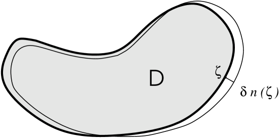
Figure 1: The normal displacement of the boundary.

As an explicitly solvable example, consider the Ginibre-Girko ensemble with the partition function (2.8). In this case the support of eigenvalues is an ellipse with the half-axes

$$a=\sqrt{t\,\frac{1+2|t_{2}|}{1-2|t_{2}|}},\quad\quad b=\sqrt{t\,\frac{1-2|t_{2}|}{1+2|t_{2}|}},$$

centered at the point $\displaystyle{z_{0}=\frac{2t_{1}\bar{t}_{2}+\bar{t}_{1}}{1-4|t_{2}|^{2}}}$, and with the angle between the big axis and the real line being equal to $\frac{1}{2}\mbox{arg}\,t_{2}$. For the model with the potential $W=-|z|^{2}+2\Re(t_{3}z^{3})$ the droplet of eigenvalues is bounded by a hypotrochoid [12].

4.3 Small deformations of the support of eigenvalues

Coming back to the general case, let us examine how the shape of ${\sf D}$ changes under a small change of the potential $W$ with $t=\hbar N$ fixed. It is convenient to describe small deformations ${\sf D}\rightarrow\tilde{\sf D}$, by the normal displacement $\delta n(\zeta)$ at a boundary point $\zeta$ (Fig. 1). Consider a small variation of the potential $W$ in the condition (4.7). To take into account the deformation of the domain, we write, for any fixed function $f$,

$$\delta\left(\oint_{\partial{\sf D}}\!\!f(\zeta)d\zeta\right)=\oint_{\partial(\delta{\sf D})}\!\!f(\zeta)d\zeta=2i\!\!\int_{\delta{\sf D}}\!\!\bar{\partial}f(\zeta)d^{2}\zeta\approx 2i\!\oint_{\partial{\sf D}}\!\!\bar{\partial}f(\zeta)\delta n(\zeta)|d\zeta|$$

(here $\delta{\sf D}=\tilde{\sf D}\setminus{\sf D}$) and thus obtain from (4.7):

$$\oint_{\partial{\sf D}}\!\!\frac{\partial\,\delta W(\zeta)d\zeta}{z-\zeta}\,+\,\frac{i}{2}\oint_{\partial{\sf D}}\!\!\frac{\Delta W(\zeta)\delta n(\zeta)}{z-\zeta}\,|d\zeta|\,=\,0.$$ (4.9)

This integral equation for $\delta n(\zeta)$ can be solved in terms of the exterior Dirichlet boundary value problem. Given any smooth function $f(z)$, let $f^{H}(z)$ be its harmonic continuation from the boundary of ${\sf D}$ to its exterior, i.e., a unique function such that $\Delta f^{H}=0$ in ${\sf D^{c}}$ and regular at $\infty$, and $f^{H}(z)=f(z)$ for all $z\in\partial{\sf D}$. Explicitly, a harmonic function can be reconstructed from its boundary value by means of the formula

$$f^{H}(z)=-\frac{1}{2\pi}\oint_{\partial{\sf D}}f(\xi)\partial_{n}G(z,\xi)|d\xi|\,.$$ (4.10)

(Here and below, $\partial_{n}$ is the normal derivative at the boundary, with the outward pointing normal vector.) The main ingredient of this formula is the Green’s function $G(z,\xi)$ of the domain ${\sf D^{c}}$ characterized by the properties $\Delta_{z}G(z,\zeta)=2\pi\delta^{(2)}(z-\zeta)$ in ${\sf D^{c}}$, $G(z,\zeta)=0$ if $z$ or $\zeta$ $\in\partial{\sf D}$. As $\zeta\to z$, it has the logarithmic singularity $G(z,\zeta)\to\log|z-\zeta|$.

Consider the integral $\displaystyle{\oint_{\partial{\sf D}}\!\!\frac{\partial(\delta W^{H}(\xi))d\xi}{z-\xi}}$ which is obviously equal to $0$ for all $z$ inside ${\sf D}$, subtract it from the first term in (4.9) and rewrite the latter as an integral over the line element $|d\xi|$. After this transformation (4.9) acquires the form

$$\frac{1}{2\pi i}\oint_{\partial{\sf D}}\frac{R(\xi)}{z-\xi}\,|d\xi|=0\quad\quad\mbox{for all $z\in{\sf D}$},$$ (4.11)

where

$$R(z)=\Delta W(z)\delta n(z)+\partial_{n}^{-}\left(\delta W(z)\!-\!(\delta W)^{H}(z)\right)$$ (4.12)

is a real-valued function on the boundary contour $\partial{\sf D}$. The superscript indicates that the derivative is taken in the exterior of the boundary. By properties of Cauchy integrals, it follows from (4.11) that $R(\xi)/\tau(\xi)$, where $\tau(\xi)=d\xi/|d\xi|$ is the unit tangential vector to the boundary curve, is the boundary value of an analytic function $h(z)$ in ${\sf D^{c}}$ such that $h(\infty)=0$. For $z\in{\sf D^{c}}$, this function is just given by the integral in the l.h.s. of (4.11). Variation of the normalization condition (the second equation in (4.6)) yields, in a similar manner:

$$\oint_{\partial{\sf D}}R(\xi)|d\xi|=0$$ (4.13)

This relation implies that the zero at $\infty$ is at least of the 2-nd order.

The following simple argument shows that an analytic function with these properties must be identically zero. Let $w(z)$ be the conformal map from ${\sf D^{c}}$ onto the unit disk such that $w(\infty)=0$ and the derivative at $\infty$ is real positive. By the well known property of conformal maps we have

$$\frac{dz}{|dz|}\,e^{i\,\mbox{{\footnotesize arg}}w^{\prime}(z)}=\frac{dw}{|dw|}$$

along the boundary curve. Therefore, $\tau(z)=i|w^{\prime}(z)|\,w(z)/w^{\prime}(z)$ and we thus see that

$$\frac{R(z)\,w^{\prime}(z)}{i|w^{\prime}(z)|w(z)}$$

is the boundary value of the holomorphic function $h(z)$. Since $w^{\prime}(z)\neq 0$ in ${\sf D^{c}}$, the function $g(z)=h(z)\,w(z)/w^{\prime}(z)$ is holomorphic there with the purely imaginary boundary value $\frac{R(z)}{i|w^{\prime}(z)|}$. Then the real part of this function is harmonic and bounded in ${\sf D^{c}}$ and is equal to $0$ on the boundary. By uniqueness of a solution to the Dirichlet boundary value problem, $\Re\,g(z)$ must be equal to $0$ identically. Therefore, $g(z)$ takes purely imaginary values everywhere in ${\sf D^{c}}$ and so is a constant. By virtute of condition (4.13) this constant must be $0$ which means that $R(z)\equiv 0$.

Therefore, one obtains the following result for the normal displacement of the boundary caused by a small change of the potential $W\rightarrow W+\delta W$:

$$\delta n(z)=\frac{\partial_{n}^{-}(\delta W^{H}(z)\!-\!\delta W(z))}{\Delta W(z)}\,.$$ (4.14)

4.4 From the support of eigenvalues to an algebraic curve

There is an interesting algebraic geometry behind the large $N$ limit of matrix models. For simplicity, here we consider models with quasiharmonic potentials.

The boundary of the support of eigenvalues is a closed curve in the plane without self-intersections. If $V^{\prime}(z)$ is a rational function, then this curve is a real section of a complex algebraic curve of finite genus. In fact, this curve encodes the $1/N$ expansion of the model. In the context of Hermitian 2-matrix model such a curve was introduced and studied in [23, 24].

To explain how the curve comes into play, we start from the equation $\partial\varphi_{0}=\partial W$, which can be written in the form $\bar{z}-V^{\prime}(z)=G(z)$ for $z\in{\sf D}$, where $\displaystyle{G(z)=\frac{1}{\pi}\int_{{\sf D}}\frac{d^{2}\zeta}{z-\zeta}}$. Clearly, this function is analytic in ${\sf D^{c}}$. At the same time, $V^{\prime}(z)$ is analytic in ${\sf D}$ and all its singularities in ${\sf D^{c}}$ are poles. Set $S(z)=V^{\prime}(z)+G(z)$. Then $S(z)=\bar{z}$ on the boundary of the support of eigenvalues. So, $S(z)$ is the analytic continuation of $\bar{z}$ away from the boundary. Assuming that poles of $V^{\prime}$ are not too close to $\partial{\sf D}$, $S(z)$ is well-defined at least in a piece of ${\sf D^{c}}$ adjacent to the boundary. The complex conjugation yields $\overline{S(z)}=z$, so the function $\bar{S}(z)=\overline{S(\bar{z})}$ must be inverse to the $S(z)$: $\bar{S}(S(z))=z$ (“unitarity condition”). The function $S(z)$ is called the Schwarz function [25].

Under our assumptions, $S(z)$ is an algebraic function, i.e., it obeys a polynomial equation $P(z,S(z))=0$ of the form

$$P(z,S(z))=\sum_{n,l=1}^{d+1}a_{nl}z^{n}(S(z))^{l}=0,$$

where $\overline{a_{ln}}=a_{nl}$ and $d$ is the number of poles of $V^{\prime}(z)$ (counted with their multiplicities). Here is a sketch of proof. Consider the Riemann surface $\mit\Sigma={\sf D^{c}}\cup\partial{\sf D}\cup({\sf D^{c}})^{*}$ (the Schottky double of ${\sf D^{c}}$). Here, $({\sf D^{c}})^{*}$ is another copy of ${\sf D^{c}}$, with the local coordinate $\bar{z}$, attached to it along the boundary. On $\mit\Sigma$, there exists an anti-holomorphic involution that interchanges the two copies of ${\sf D^{c}}$ leaving the points of $\partial{\sf D}$ fixed. The functions $z$ and $S(z)$ are analytically extendable to $({\sf D^{c}})^{*}$ as $\overline{S(z)}$ and $\bar{z}$ respectively. We have two meromorphic functions, each with $d+1$ poles, on a closed Riemann surface. Therefore, they are connected by a polynomial equation of degree $d+1$ in each variable. Hermiticity of the coefficients follows from the unitarity condition.

The polynomial equation $P(z,\tilde{z})=0$ defines a complex curve $\mit\Gamma$ with anti-holomorphic involution $(z,\tilde{z})\mapsto(\overline{\tilde{z}},\bar{z})$. The real section is the set of points such that $\tilde{z}=\bar{z}$. It is the boundary of the support of eigenvalues.

It is important to note that for models with non-Gaussian weights (in particular, with polynomial potentials of degree greater than two) the curve has a number of singular points, although the Riemann surface $\mit\Sigma$ (the Schottky double) is smooth. Generically, these are double points, i.e., the points where the curve crosses itself. In our case, a double point is a point $z^{(d)}\in{\sf D^{c}}$ such that $S(z^{(d)})=\overline{z^{(d)}}$ but $z^{(d)}$ does not belong to the boundary of ${\sf D}$. Indeed, this condition means that two different points of $\mit\Sigma$, connected by the antiholomorphic involution, are stuck together on the curve $\mit\Gamma$, which means self-intersection. The double points play the key role in deriving the nonperturbative (instanton) corrections to the large $N$ matrix models results (see [26] for details).

4.5 Free energy and correlation functions

Free energy.

The leading contribution to the free energy in the large $N$ limit is

$$F_{0}=\lim_{\hbar\to 0}\left(\hbar^{2}\log Z_{N}\right).$$

It is determined by the maximal value of the integrand in (2.9), i.e., by the extremum of the function $E$. In the continuous approximation, one can represent it as a functional of the density:

$$-\beta\hbar^{2}E[\rho]=\beta\int\!\!\int\rho(z)\rho(\zeta)\log|z-\zeta|d^{2}zd^{2}\zeta\,+\,\int W(z)\rho(z)d^{2}z$$ (4.15)

and find its minimum with the constraint $\int\rho\,d^{2}z=t$. Introducing a Lagrange multiplier $\lambda$, we get the equation

$$2\beta\int\log|z-\zeta|\rho(\zeta)d^{2}\zeta+W(z)+\lambda=0$$

which is solved, as expected, by the function $\rho_{0}$ discussed in section 4.1. Assuming that $W(0)=0$, we find $\lambda=\varphi_{0}(0)$ and

$$F_{0}=-\beta E[\rho_{0}]=-\frac{1}{\beta}\int_{{\sf D}}\!\!\int_{{\sf D}}\sigma(z)\log\left|\frac{1}{z}\!-\!\frac{1}{\zeta}\right|\sigma(\zeta)d^{2}zd^{2}\zeta\,.$$ (4.16)

Some results for correlation functions.

Here are some results for the correlation functions obtained by the variational technique. (For details of the derivation see [10].) They are correct at distances much larger than the mean distance between the charges. The leading contribution to the one-trace function was already found in Section 4.1:

$$\begin{array}[]{c}\left<\mbox{tr}f(\Phi)\right>\,\,=\,\,\displaystyle{\frac{1}{\hbar\beta}\int_{{\sf D}}\sigma(z)f(z)\,d^{2}z}+O(1).\end{array}$$ (4.17)

The connected two-trace function is:

$$\left<\mbox{tr}\,f(\Phi)\,\mbox{tr}\,g(\Phi)\right>_{c}=\frac{1}{4\pi\beta}\int_{{\sf D}}\nabla f\nabla gd^{2}z-\frac{1}{4\pi\beta}\oint_{\partial{\sf D}}f\partial_{n}g^{H}|dz|+O(\hbar)$$ (4.18)

(here $\nabla f\nabla g=\partial_{x}f\partial_{x}g+\partial_{y}f\partial_{y}g$). In particular, for the connected correlation functions of the fields $\varphi(z)$ this formula gives:

$$\!\!\!\left<\varphi(z)\varphi(z^{\prime})\right>_{{\rm c}}\!=\!\!\left\{\begin{array}[]{l}\displaystyle{\!\!-2\beta\hbar^{2}\,\log\frac{|z-z^{\prime}|}{r}+O(\hbar^{3})\quad\,\,\mbox{inside}\,\,{\sf D}}\\ \\ \displaystyle{\!\!2\beta\hbar^{2}\!\left(G(z,z^{\prime})\!-\!G(z,\infty)\!-\!G(z^{\prime},\infty)\!-\!\log\frac{|z\!-\!z^{\prime}|}{r}\right)\!+\!O(\hbar^{3})\,\,\,\mbox{outside}\,\,{\sf D}}\end{array}\right.$$ (4.19)

where $G$ is the Green’s function of the Dirichlet boundary value problem and

$${r=\exp\Bigl{[}\lim_{\xi\to\infty}(\log|\xi|+G(\xi,\infty))\Bigr{]}}$$ (4.20)

is the external conformal radius of the domain ${\sf D}$ (the Robin’s constant). This result is valid if $|z-z^{\prime}|\gg\sqrt{\hbar}$. The 2-trace functions are universal, i.e., they depend on the shape of the support of eigenvalues only and do not depend on the potential $W$ explicitly. They resemble the two-point functions of the Hermitian 2-matrix model found in [27]; they were also obtained in [28] in the study of thermal fluctuations of a confined 2D Coulomb gas. The structure of the formulas indicates that there are local correlations in the bulk as well as strong long range correlations at the edge of the support of eigenvalues. (See [29] for a similar result in the context of classical Coulomb systems).

5 The matrix model as a growth problem

5.1 Growth of the support of eigenvalues

When $N$ increases at a fixed potential $W$, one may say that the support of eigenvalues grows. More precisely, we are going to find how the shape of the support of eigenvalues changes under $t\rightarrow t+\delta t$, where $t=N\hbar$, if $W$ stays fixed.

The starting point is the same as for the variations of the potential, and the calculations are very similar as well. Variation of the conditions (4.6) yields

$$\oint_{\partial{\sf D}}\frac{\Delta W(\zeta)\delta n(\zeta)}{z-\zeta}\,|d\zeta|=0\;\;\;\mbox{for all $z\in{\sf D}$},\;\;\;\;\;\oint_{\partial{\sf D}}\Delta W(\zeta)\delta n(\zeta)\,|d\zeta|=-4\pi\beta\delta t\,.$$

The first equation means that $\Delta W(z)\delta n(z)\frac{|dz|}{dz}$ is the boundary value of an analytic function $h(z)$ such that $h(z)=-4\pi\beta\delta t/z+O(z^{-2})$ as $z\to\infty$. The solution for the $\delta n(z)$ is again expressed in terms of the Green’s function in ${\sf D^{c}}$:

$$\delta n(z)=-\,\frac{\beta\delta t}{2\pi\sigma(z)}\,\partial_{n}G(\infty,z).$$ (5.1)

For quasiharmonic potentials (with $\sigma=1/\pi$), the formula simplifies:

$$\delta n(z)=-\frac{\beta}{2}\,\delta t\,\partial_{n}G(\infty,z).$$ (5.2)

Identifying $t$ with time, one can say that the normal velocity of the boundary at any point $z$, $V_{n}(z)=\delta n(z)/\delta t$, is proportional to gradient of the Green’s function: $V_{n}(z)\propto-\partial_{n}G(\infty,z)$.

If the domain is connected, $G$ can be expressed through the conformal map $w(z)$ from ${\sf D^{c}}$ onto the exterior of the unit circle:

$$G(z_{1},z_{2})=\log\left|\frac{w(z_{1})-w(z_{2})}{1-w(z_{1})\overline{w(z_{2})}}\right|.$$ (5.3)

In particular, $G(\infty,z)=-\log|w(z)|$. As $|z|\to\infty$, $w(z)=z/r+O(1)$, where $r$ is the Robin’s constant which enters eq. (4.19). It is easy to see that $\partial_{n}\log|w(z)|=|w^{\prime}(z)|$ on $\partial{\sf D}$, so one can rewrite the growth law (5.2) as $\delta n(z)=\frac{\beta}{2}\,|w^{\prime}(z)|\,\delta t$.

5.2 Laplacian growth

The growth law (5.2) is common to many important problems in physics. The class of growth processes, in which dynamics of a moving front (an interface) between two distinct phases is driven by a harmonic scalar field is known under the name Laplacian growth. The most known examples are viscous flows in the Hele-Shaw cell, filtration processes in porous media, electrodeposition and solidification of undercooled liquids. A comprehensive list of relevant papers published prior to 1998 can be found in [16].

Viscous flows in Hele-Shaw cell.

To be specific, we shall speak about an interface between two incompressible fluids with very different viscosities on the plane (say, oil and water). In practice, the 2D geometry is realized in the Hele-Shaw cell – a narrow gap between two parallel glass plates. For a review, see [14, 15]. The velocity field in a viscous fluid in the Hele-Shaw cell is proportional to the gradient of pressure $p$ (Darcy’s law):

$$\vec{V}=-K\nabla p\,,\;\;\;\;K=\frac{b^{2}}{12\mu}\,.$$

The constant $K$ is called the filtration coefficient, $\mu$ is viscosity and $b$ is the size of the gap between the two plates. Note that if $\mu\to 0$, then $\nabla p\to 0$, i.e., pressure in a fluid with negligibly small viscosity is uniform. Incompressibility of the fluids ($\nabla\vec{V}=0$) implies that the pressure field is harmonic: $\Delta p=0$. By continuity, the velocity of the interface between the two fluids is proportional to the normal derivative of the pressure field on the boundary: $V_{n}=-K\partial_{n}p$.

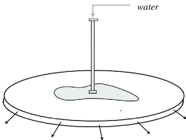
Figure 2: The Hele-Shaw cell.

To be definite, we assume that the Hele-Shaw cell contains a bounded droplet of water surrounded by an infinite “sea” of oil (another possible experimental set-up is an air bubble surrounded by oil or water). Water is injected into the droplet while oil is withdrawn at infinity at a constant rate, as is shown schematically in Fig. 2. The latter means that the pressure field behaves as $p\propto-\log|z|$ at large distances. We also assume that the interface is a smooth closed curve $\Gamma$. As it is mentioned above, one may set $p=0$ inside the water droplet. However, pressure usually has a jump across the interface, so $p$ in general does not tend to zero if one approaches the boundary from outside. This effect is due to surface tension. It is hard to give realistic estimates of the surface tension effect from fundamental principles, so one often employs certain ad hoc assumptions. The most popular one is to say that the pressure jump is proportional to the local curvature, $\kappa$, of the interface.

To summarize, the mathematical setting of the Saffman-Taylor problem is as follows:

$$\left\{\begin{array}[]{ll}V_{n}=-\partial_{n}p&\quad\mbox{on $\Gamma$}\\ \Delta p=0&\quad\mbox{in oil}\\ p\to-\log|z|&\quad\mbox{in oil as $|z|\to\infty$}\\ p=0&\quad\mbox{in water}\\ p^{(+)}-p^{(-)}=-\nu\kappa&\quad\mbox{across $\Gamma$}\end{array}\right.$$ (5.4)

Here $\nu$ is the surface tension coefficient. (The filtration coefficient is set to be $1$.) The experimental evidence suggests that when $\nu$ is small enough, the dynamics becomes unstable. Any initial domain develops an unstable fingering pattern. The fingers split into new ones, and after a long lapse of time the water droplet attains a fractal-like structure. This phenomenon is similar to the formation of fractal patterns in the diffusion-limited aggregation.

Comparing (5.2) and (5.4), we identify ${\sf D}$ and ${\sf D^{c}}$ with the domains occupied by water and oil respectively, and conclude that the growth laws are identical, with the pressure field being given by the Green function: $p(z)=G(\infty,z)$, and $p=0$ on the interface. The latter means that supports of eigenvalues grow according to (5.4) with zero surface tension, i.e., with $\nu=0$ in (5.4). Neglecting the surface tension effects, one obtains a good approximation unless the curvature of the interface becomes large. We see that the idealized Laplacian growth problem, i.e., the one with zero surface tension, is mathematically equivalent to the growth of the support of eigenvalues in ensembles of random matrices ${\cal N}$ or ${\cal C}$ and in general $\beta$-ensembles.

Finite-time singularities as critical points.

As a matter of fact, the Laplacian growth problem with zero surface tension is ill-posed since an initially smooth interface often becomes singular in the process of evolution, and the solution blows up. The role of surface tension is to inhibit a limitless increase of the interface curvature. In the absence of such a cutoff, the tip of the most rapidly growing finger typically grows to a singularity (a cusp). In particular, a singularity necessarily occurs for any initial interface that is the image of the unit circle under a rational conformal map, with the only exception of an ellipse.

An important fact is that the cusp-like singularity occurs at a finite time $t=t_{c}$, i.e., at a finite area of the droplet. It can be shown that the conformal radius of the droplet $r$ (as well as some other geometric parameters), as $t\to t_{c}$, exhibits a singular behavior

$$r-r_{c}\propto(t_{c}-t)^{-\gamma}$$

characterized by a critical exponent $\gamma$. The generic singularity is the cusp $(2,3)$, which in suitable local coordinates looks like $y^{2}=x^{3}$. In this case $\gamma=-\frac{1}{2}$.

A similar phenomenon has been known in the theory of random matrices for quite a long time, and in fact it was the key to their applications to 2D quantum gravity and string theory. In the large $N$ limit, the random matrix models have critical points – the points where the free energy is not analytic as a function of a coupling constant. As we have seen, the Laplacian growth time $t$ should be identified with a coupling constant of the normal or complex matrix model. In a vicinity of a critical point,

$$F_{0}\sim F_{0}^{{\rm reg}}\,+\alpha(t_{c}-t)^{2-\gamma},$$

where the critical index $\gamma$ (often denoted by $\gamma_{{\rm str}}$ in applications to string theory) depends on the type of the critical point. Accordingly, the singularities show up in correlation functions. Using the equivalence established above, we can say that the finite-time blow-up (a cusp-like singularity) of the Laplacian growth with zero surface tension is a critical point of the normal and complex matrix models. Remarkably, the evolution can be continued to the post-critical regime as a dynamics of “shock lines” [30].

References

- [1] M.L.Mehta, Random matrices and the statistical theory of energy levels, 2-nd edition, Academic Press, NY, 1991
- [2] T.Guhr, A.Müller-Groeling and H.Weidenmüller, Phys. Rep. 299 (1998) 189-428, e-print archive: cond-mat/9707301
- [3] P.Di Francesco, P.Ginsparg and J.Zinn-Justin, Phys. Rep. 254 (1995) 1-133
- [4] A.Morozov, Phys. Usp. 37 (1994) 1-55, e-print archive: hep-th/9303139
- [5] Y.Fyodorov, B.Khoruzhenko and H.-J.Sommers, Phys. Rev. Lett. 79 (1997) 557, e-print archive: cond-mat/9703152; J.Feinberg and A.Zee, Nucl. Phys. B504 (1997) 579-608, e-print archive: cond-mat/9703087; G.Akemann, J. Phys. A 36 (2003) 3363, e-print archive: hep-th/0204246; G.Akemann, Phys. Rev. Lett. 89 (2002) 072002, e-print archive: hep-th/0204068 A.M.Garcia-Garcia, S.M.Nishigaki and J.J.M.Verbaarschot, Phys. Rev. E66 (2002) 016132 e-print archive: cond-mat/0202151
- [6] J.Ginibre, J. Math. Phys. 6 (1965) 440
- [7] L.Chau and Y.Yu, Phys. Lett. A167 (1992) 452-458; L.Chau and O.Zaboronsky, Commun. Math. Phys. 196 (1998) 203
- [8] F.Dyson, J. Math. Phys. 3 (1962) 140, 157, 166
- [9] I.Kostov, I.Krichever, M.Mineev-Weinstein, P.Wiegmann and A.Zabrodin, -function for analytic curves, Random matrices and their applications, MSRI publications, eds. P.Bleher and A.Its, vol.40, p. 285-299, Cambridge Academic Press, 2001, e-print archive: hep-th/0005259
- [10] P.Wiegmann and A.Zabrodin, J. Phys. A 36 (2003) 3411, e-print archive: hep-th/0210159
- [11] A.Zabrodin, Ann. Henri Poincaré 4 Suppl. 2 (2003) S851-S861, e-print archive: cond-mat/0210331
- [12] R.Teodorescu, E.Bettelheim, O.Agam, A.Zabrodin and P.Wiegmann, Nucl. Phys. B704/3 (2005) 407-444, e-print archive: hep-th/0401165; Nucl. Phys. B700 (2004) 521-532, e-print archive: hep-th/0407017
- [13] A.Zabrodin, Matrix models and growth processes: from viscous flows to the quantum Hall effect, arXiv:hep-th/0412219, in: “Applications of Random Matrices in Physics”, pp. 261-318, Ed. E.Brezin et al, Springer, 2006
- [14] D.Bensimon, L.P.Kadanoff, S.Liang, B.I.Shraiman, and C.Tang, Rev. Mod. Phys. 58 (1986) 977
- [15] B. Gustafsson, A. Vasil’ev, Conformal and Potential Analysis in Hele-Shaw Cells, Birkhäuser Verlag, 2006.
- [16] K.A.Gillow and S.D.Howison, A bibliography of free and moving boundary problems for Hele-Shaw and Stokes flow, http://www.maths.ox.ac.uk/ howison/Hele-Shaw/
- [17] V.Girko, Theor. Prob. Appl. 29 (1985) 694
- [18] P.Di Francesco, M.Gaudin, C.Itzykson and F.Lesage, Int. J. Mod. Phys. A9 (1994) 4257-4351
- [19] P.Elbau and G.Felder, Density of eigenvalues of random normal matrices, e-print archive: math.QA/0406604
- [20] H.Hedenmalm and N.Makarov, Quantum Hele-Shaw flow, e-print archive: math.PR/0411437
- [21] F.Balogh and J.Harnad, Superharmonic perturbations of a Gaussian measure, equilibrium measures and orthogonal polynomials, To appear in: Complex Analysis and Operator Theory (Special volume in honour of Bjorn Gustafsson), e-print archive: arXiv:0808.1770
- [22] P.J.Forrester, Physics Reports, 301 (1998) 235-270; Log gases and random matrices webpage http://www.ms.unimelb.edu.au/ matjpf/matjpf.html
- [23] M.Staudacher, Phys. Lett B305 (1993) 332-338, e-print archive: hep-th/9301038
- [24] V.Kazakov and A.Marshakov, J. Phys. A 36 (2003) 3107, e-print archive: hep-th/0211236
- [25] P.J.Davis, The Schwarz function and its applications, The Carus Math. Monographs, No. 17, The Math. Assotiation of America, Buffalo, N.Y., 1974
- [26] F.David, Phys. Lett. B302 (1993) 403-410, e-print archive: hep-th/9212106; B.Eynard and J.Zinn-Justin, Phys. Lett. B302 (1993) 396-402, e-print archive: hep-th/9301004; V.Kazakov and I.Kostov, e-print archive: hep-th/0403152; S.Alexandrov, JHEP 0405 (2004) 025, e-print archive: hep-th/0403116
- [27] J.-M.Daul, V.Kazakov and I.Kostov, Nucl. Phys. B409 (1993) 311
- [28] A.Alastuey and B.Jancovici, J. Stat. Phys. 34 (1984) 557; B.Jancovici J. Stat. Phys. 80 (1995) 445
- [29] B.Jancovici, J. Stat. Phys. 28 (1982) 43
- [30] S.-Y.Lee, R.Teodorescu and P.Wiegmann, Shocks and finite-time singularities in Hele-Shaw flow, Physica D238 (2009) 1113-1128