IFT-UAM/CSIC-09-31

Matter wave functions and Yukawa couplings in
F-theory Grand Unification
A. Font¹ and L.E. Ibáñez^2
1 Departamento de Física, Centro de Física Teórica y Computacional
Facultad de Ciencias, Universidad Central de Venezuela
A.P. 20513, Caracas 1020-A, Venezuela
² Departamento de Física Teórica and Instituto de Física Teórica UAM-CSIC,
Universidad Autónoma de Madrid, Cantoblanco, 28049 Madrid, Spain
Abstract

We study the local structure of zero mode wave functions of chiral matter fields in F-theory unification. We solve the differential equations for the zero modes derived from local Higgsing in the 8-dimensional parent action of F-theory 7-branes. The solutions are found as expansions both in powers and derivatives of the magnetic fluxes. Yukawa couplings are given by an overlap integral of the three wave functions involved in the interaction and can be calculated analytically. We provide explicit expressions for these Yukawas to second order both in the flux and derivative expansions and discuss the effect of higher order terms. We explicitly describe the dependence of the couplings on the $U(1)$ charges of the relevant fields, appropriately taking into account their normalization. A hierarchical Yukawa structure is naturally obtained. The application of our results to the understanding of the observed hierarchies of quarks and leptons is discussed.

1 Introduction

The hierarchical structure of fermion masses and mixings is one of the most remarkable properties of the Standard Model (SM). An outstanding challenge of string theory compactifications is to obtain models with the massless spectrum of the SM and reproducing naturally such hierarchical structure. In type IIB orientifold, as well as heterotic, compactifications the Yukawa couplings which govern fermion masses and mixings are in principle calculable, in the large compact volume limit, in terms of overlap integrals [1, 2]

$$Y_{ij}\ =\ \int_{X_{3}}\ \!\!\psi_{i}\,\psi_{j}\,\phi_{H}$$ (1.1)

Here $\psi_{i}$ and $\phi_{H}$ are internal wave functions associated to the fermions and Higgs fields respectively, taking values in the compact complex threefold $X_{3}$. These wave functions are zero modes of higher dimensional fields in the compact internal space. The technical problem here is that in general we do not know how to compute the relevant wave functions for arbitrary curved spaces $X_{3}$. Such a computation has been completely worked out for the relatively simple case of type IIB toroidal orientifolds [3] with constant $U(1)$ fluxes (see also [4, 5, 6]). In this case with a flat geometry the equations of motion can be fully solved to obtain the wave functions which turn out to have a neat expression in terms of Jacobi $\vartheta$-functions. It was found that in the simplest models only one generation of quarks and leptons acquires a non-trivial Yukawa coupling, which is a good starting point to reproduce the observed hierarchies [3]. Having explicit solutions for the wave functions is also useful to study other physical properties of the compactifications such as the effect of closed string fluxes and warping [7].

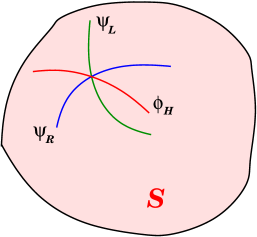
Figure 1: Intersecting matter curves

Clearly, it would be interesting to obtain wave functions and Yukawa couplings in more complicated curved geometries and for non-constant fluxes. An obvious obstruction is that determining the wave functions seems to require a knowledge of the global geometry of the compact $X_{3}$ manifold. In fact, the problem may be more tractable within the context of a bottom-up approach as advocated in [8] (see also [9, 10, 11, 12]). The idea is that in order to extract the relevant physics of a SM compactification it is enough to have a local description of the geometry of the branes in which the SM fields reside. This is the case for example of models derived from D3-branes at singularities [8, 9, 11] in which the SM physics only depends on the local geometry around the singularity. This type of structure is also characteristic of local configurations of D7-branes wrapping intersecting 4-cycles inside $X_{3}$. F-theory [13] is the natural non-perturbative extension of these local 7-brane configurations. In the last year local F-theory GUT constructions have been proposed [14, 15, 16] as a particularly attractive class of bottom-up configurations with a number of phenomenological virtues (see [17, 18, 19, 20, 21, 22, 23, 24, 25, 26, 27, 28, 29, 30, 31], as well as [32, 33, 34, 35, 36, 37, 38, 39, 40, 41, 42, 43] for other recent developments). In this scheme the Yukawa couplings arise again as overlap integrals now of the form

$$Y_{ij}\ =\ \int_{S}\ \psi_{i}\,\psi_{j}\,\phi_{H}$$ (1.2)

in which $S$ is the compact complex twofold wrapped by the GUT F-theory 7-brane. The quark and lepton multiplets of the SM reside at matter Riemann curves $\Sigma_{I}$ inside $S$, which correspond geometrically to the intersection of $S$ with the world-volume of other $U(1)$ 7-branes. Yukawa couplings come from the triple overlap of these matter curves involving quarks, leptons and Higgs fields (see figure 1). In order to compute the Yukawa coupling (1.2) we need again the internal wave functions. However, in this case given the local geometry of the coupling it would be enough to have a knowledge of the wave functions close to the intersection point. It was pointed out in [15] that one can determine the profile of these wave functions close to the intersection point in terms of a certain quasi-topological theory in $D$=8. The equations of motion of that theory have solutions corresponding to hypermultiplet zero modes localized along the matter curves with a Gaussian profile. One finds [19] that to leading order, for a compactification having three generations, only one of them gets a non-trivial Yukawa, in analogy with the results in [3]. However the distortion of the wave functions, due to the presence of $U(1)$ gauge fluxes, could be the natural source of the observed hierarchy of masses and mixings of quarks and leptons [19].

In this article we make a systematic study of the solutions of the differential equations of motion of the quasi-topological $D$=8 theory of [15]. The zero mode solutions give the local wave functions corresponding to the massless particles residing at the matter curves of F-theory unification models. We make an expansion both in powers and derivatives of the $U(1)$ fluxes and explicitly solve the differential equations. Equipped with these wave functions we compute the Yukawa couplings from the overlap integral of the three wave functions involved in the couplings. These integrals may be calculated analytically and we provide explicit expressions for these Yukawa couplings up to fourth order in the flux and derivative expansions. As suggested in [19], a hierarchy of masses for fermions naturally appears. We also study the application of our results to the understanding of the observed hierarchy of masses and mixings in the SM. We find good qualitative agreement with experiment for reasonable ranges of the flux parameters.

The organization of the rest of this article is as follows. In the next section we provide a brief review of the aspects of F-theory models that concern our discussion. In chapter 3 we study the wave functions of the zero modes which are solutions of the quasi-topological $D$=8 field theory equations. We consider both constant and varying fluxes in a general setting of three intersecting matter curves. The details of the solutions are given in appendix A. In chapter 4 we address the explicit computation of the Yukawa couplings by evaluating the overlap integral of the three relevant wave functions. Based on the leading terms in the Yukawa couplings provided in appendix B, we describe the general structure of the flux-induced corrections and their contribution to the Yukawa matrices. In chapter 5 we apply the previous results to the analysis of the fermion mass spectra of $SU(5)$ GUT’s with non-vanishing hypercharge flux breaking the theory down to the SM. We show that reasonable agreement with observed mass hierarchies and mixing may be obtained for appropriate flux parameters. Chapter 6 is devoted to some final comments and discussion.

The computation of Yukawa couplings in analogous settings has been more recently analyzed in [49, 50], see the note added at the end of this paper.

2 Review of F-theory unification

The purpose of this section is to give a short overview of the F-theory formalism developed in [15] (see also [14, 17]).

In the F-theory setup, the $D$=4 supersymmetric gauge theory descends from 7-branes wrapping a compact surface $S$ of complex codimension one in the threefold base of an elliptically-fibered Calabi-Yau fourfold. The gauge group $G_{S}$ on the 7-branes depends on the singularity type of the elliptic fiber. In turn $G_{S}$ can be broken by a vev in a subgroup $H_{S}\subset G_{S}$. We consider $H_{S}=U(1)$, typical examples being the hypercharge in $SU(5)$ or $U(1)_{B-L}$ in an $SO(10)$ GUT. The $U(1)$ background breaks the gauge group and gives rise to matter charged under the commutant of $H_{S}$ in $G_{S}$. We assume that $S$ is a del Pezzo surface so that gravity decouples from the gauge theory [15].

The singularity type of the elliptic fiber can be enhanced to group $G_{\Sigma}$ along a curve $\Sigma\subset S$ of complex codimension two on the threefold base. This curve appears at the intersection of $S$ and another surface $S^{\prime}$. On the 7-branes wrapping $S^{\prime}$ there is a gauge theory with group $G_{S^{\prime}}$ which decouples when $S^{\prime}$ is non-compact. Based on the knowledge of intersecting D-branes, one expects additional degrees of freedom due to open strings stretching between the 7-branes wound on $S$ and $S^{\prime}$. The extra fields localized on the matter curve $\Sigma$ must be charged under $G_{S}\times G_{S^{\prime}}$. Indeed this is the picture that arises in F-theory [44, 15].

We will now review the basic facts about the charged fields originating in the surface $S$ and in the matter curve $\Sigma$. Our discussion is brief and follows mostly [15].

2.1 Bulk fields

The effective physics of the 7-branes wrapping $S$ is described by $D$=8 twisted super Yang-Mills on $\mathbbm{R}^{3,1}\times S$ [15]. The supersymmetric multiplets include the gauge field, plus a complex scalar $\varphi$ and fermions $(\eta,\psi,\chi)$ in the adjoint. After twisting the scalar and fermions become forms on $S$. Using local coordinates $(z_{1},z_{2})$ for $S$ the results are summarized by

$$A=A_{\mu}dx^{\mu}+A_{m}dz^{m}+A_{\bar{m}}d{\bar{z}}^{m}\quad \quad\varphi=\varphi_{12}\,dz^{1}\wedge dz^{2}$$ ;

$$\psi_{\alpha}=\psi_{\alpha\bar{1}}\,d\bar{z}^{1}+\psi_{\alpha\bar{2}}\,d\bar{z}^{2}\quad \quad\chi_{\alpha}=\chi_{\alpha 12}\,dz^{1}\wedge dz^{2}$$ ; (2.1)

Notice that $\psi$ is a (0,1) form whereas $\varphi$ and $\chi$ are (2,0) forms. The remaining fermion $\eta_{\alpha}$ is a (0,0) form. The subscript $\alpha$, which corresponds to left handed fermions in $\mathbbm{R}^{3,1}$, will be dropped hereafter. The $D$=4, ${\mathcal{N}}$=1 theory has gauge multiplet $(A_{\mu},\eta)$, together with chiral multiplets $(A_{\bar{m}},\psi_{\bar{m}})$ and $(\varphi_{12},\chi_{12})$, plus their complex conjugates.

The $D$=8 effective action found in [15] can be integrated over the compact surface $S$ to obtain the dynamics of the $D$=4 multiplets. In computing couplings of the charged fields the most interesting term will be the superpotential

$$W=M_{*}^{4}\int_{S}{\rm Tr\,}({\boldsymbol{F}_{S}^{(0,2)}}\wedge{\boldsymbol{\Phi}})=M_{*}^{4}\int_{S}{\rm Tr\,}({\bar{\partial}}{\boldsymbol{A}}\wedge{\boldsymbol{\Phi}})\,+\,M_{*}^{4}\int_{S}{\rm Tr\,}({\boldsymbol{A}}\wedge{\boldsymbol{A}}\wedge{\boldsymbol{\Phi}})$$ (2.2)

where $M_{*}$ is the mass scale characteristic of the supergravity limit of F-theory. Here $\boldsymbol{A}$ and $\boldsymbol{\Phi}$ are chiral superfields with components

$${\boldsymbol{A}}_{\bar{m}} = A_{\bar{m}}+\sqrt{2}\theta\psi_{\bar{m}}+\cdots$$

$${\boldsymbol{\Phi}}_{12} = \varphi_{12}+\sqrt{2}\theta\chi_{12}+\cdots$$ (2.3)

where $\cdots$ involves auxiliary fields. Only the (0,2) component of the superstrength appears in (2.3).

The equations of motion derived from the $D$=8 effective action are the starting point to discuss the zero modes. The part of the action bilinear in fermions, without kinetic terms, is found to be [15]

$$I_{F}=\int_{\mathbbm{R}^{3,1}\times S}d^{4}x\ {\rm Tr\,}\big{(}\chi\wedge\partial_{A}\psi+2i\sqrt{2}\omega\wedge\partial_{A}\eta\wedge\psi+\frac{1}{2}\psi\wedge[\varphi,\psi]+\sqrt{2}\eta[\bar{\varphi},\chi]+{\rm h.c.}\big{)}$$ (2.4)

where $\omega$ is the fundamental form of $S$. Taking variations with respect to $\eta$, $\psi$ and $\chi$ respectively gives the equations of motion

$$\omega\wedge\partial_{A}\psi+\frac{i}{2}[\bar{\varphi},\chi]=0$$ (2.5)

$$\bar{\partial}_{A}\chi-2i\sqrt{2}\omega\wedge\partial\eta-[\varphi,\psi]=0$$ (2.6)

$$\bar{\partial}_{A}\psi-\sqrt{2}[\bar{\varphi},\eta]=0$$ (2.7)

For the bosonic fields it is found that the field strength $F_{S}$ must have vanishing (2,0) and (0,2) components and verify the BPS condition

$$\omega\wedge F_{S}+\frac{i}{2}[\varphi,\bar{\varphi}]=0$$ (2.8)

Finally, the complex scalar must satisfy the holomorphicity condition $\bar{\partial}_{A}\varphi=0$.

To determine the charged massless multiplets in $D$=4 it is necessary to specify the background for the adjoint scalar $\varphi$ and the gauge field. When $\langle\varphi\rangle=0$, the equations of motion imply that the number of zero modes of $\psi$ and $\chi$ are counted by topological invariants that depend both on $S$ and the gauge bundle of the background [15].

2.2 Fields at intersections

We now want to discuss the degrees of freedom localized on a matter curve $\Sigma$ occurring at the intersection of surfaces $S$ and $S^{\prime}$. As explained in [15], to preserve ${\mathcal{N}}$=1 supersymmetry in $D$=4, the theory on $\mathbbm{R}^{3,1}\times\Sigma$ must be $D$=6 twisted super Yang-Mills. The $D$=6 twisted supermultiplet, which includes two complex scalars and a Weyl spinor, decomposes into $D$=4 chiral multiplets $(\sigma,\lambda)$ and $(\sigma^{c},\lambda^{c})$, plus CPT conjugates. The number of zero modes is given by topological invariants depending on $\Sigma$ and the gauge bundle on a background in $G_{\Sigma}$.

There is a very nice intuitive way of understanding the matter localized at $\Sigma$. The idea, originally given in [44] and expanded in [15], is to start from the $D$=8 theory on $S$ with gauge group $G_{\Sigma}$ and then turn on a background for the adjoint scalar given by

$$\langle\varphi\rangle=m^{2}z_{1}Q_{1}$$ (2.9)

where $z_{1}$ is a complex coordinate on $S$, and $Q_{1}$ is a $U(1)_{1}$ generator in the Cartan subalgebra of $G_{\Sigma}$. To streamline notation, $\varphi=\varphi_{12}$. We have explicitly introduced a mass parameter $m$ so that $\varphi$ has the standard dimensions. The basic idea is that in presence of $\langle\varphi\rangle$ the $D$=8 fields have zero modes localized at $z_{1}=0$ that are naturally associated to the fields at the intersection.

When $z_{1}=0$ the gauge group is unbroken, but when $z_{1}\not=0$ the group is broken to $G_{S}\times U(1)_{1}$, with $G_{S}$ being the group whose generators commute with $Q_{1}$. The locus $z_{1}=0$ defines the curve $\Sigma$. Thus, on $\Sigma$ the singularity enhances from $G_{S}$ to $G_{\Sigma}\supset G_{S}\times U(1)_{1}$. The breaking of the gauge group is explained by the deformation of the singularity type from $G_{\Sigma}$ to $G_{S}$ due to the background in the Cartan subalgebra [44].

For ordinary D7-branes the adjoint scalar corresponds to degrees of freedom in the transverse direction and a non-zero vev means that some branes are separated and the gauge group is broken. For instance, if there are $(K+1)$ D7-branes to begin and one is moved away, the original $SU(K+1)$ is broken to $SU(K)\times U(1)$. Furthermore, the open strings stretching between the two stacks of D7-branes give rise to massless bifundamentals $({\boldsymbol{K}},-1)+(\overline{\boldsymbol{K}},1)$ localized at the intersection. For F-theory seven-branes wrapping a surface $S$ one then expects $\langle\varphi\rangle$ to break the original gauge group to some $G_{S}$. Moreover, there will be massless ‘bifundamentals’ descending from the adjoint of $G_{\Sigma}$ which decomposes as a direct sum of irreducible representations $({\boldsymbol{R}},q_{1})$ under $G_{S}\times U(1)_{1}$.

Several examples of singularity resolution were worked out in [44] and more recently in [15, 16, 34]. For illustration let us consider the case $G_{\Sigma}=E_{6}$ and $G_{S}=SO(10)$ that will be of interest later on. Under $SO(10)\times U(1)$ the $E_{6}$ adjoint decomposes as

$${\bf 78}=({\bf 45},0)+({\bf 1},0)+({\bf 16},1)+({\bf\overline{16}},-1)$$ (2.10)

Therefore, there will be chiral multiplets transforming as ${\bf 16}$ and ${\bf\overline{16}}$ of $SO(10)$. To see how $SO(10)$ is enhanced to $E_{6}$ on $\Sigma$ it is convenient to represent the Cartan generators as vectors $|Q_{i}\rangle$ so that $|\varphi\rangle\propto z_{1}|Q_{1}\rangle$ corresponds to the adjoint vev [44]. The simple roots are elements $\langle v_{j}|$ of the dual space. Those roots with $\langle v_{j}|\varphi\rangle=0$ remain as $SO(10)$ roots while those with $\langle v_{j}|\varphi\rangle\propto z_{1}$ become the weights of the ${\bf 16}$ and ${\bf\overline{16}}$.

The resolution of the singularity by the adjoint vev can be figured out as explained in [44]. The generic $E_{6}$ singularity can be cast as [45, 15]

$$y^{2}=x^{3}+\frac{1}{4}z^{4}+\epsilon_{2}xz^{2}+\epsilon_{5}xz+\epsilon_{6}z^{2}+\epsilon_{8}x+\epsilon_{9}z+\epsilon_{12}$$ (2.11)

where the $\epsilon_{i}$ are functions that depend on the adjoint vev. More precisely, in [45] they are given in terms of an arbitrary vector $(t_{1},\cdots,t_{6})$ in the $E_{6}$ Cartan subalgebra. In our notation, in the $E_{6}\supset SO(10)\times U(1)_{1}$ example, $t_{1}=z_{1}$ while other $t_{i}$’s vanish. By choosing $t_{1}=-3t$, and computing the $\epsilon_{i}$ according to the formulas of [45], we obtain the deformation

$$y^{2}=x^{3}+\frac{1}{4}z^{4}-3t^{2}xz^{2}-12t^{5}xz-6t^{6}z^{2}-12t^{8}x-16t^{9}z-12t^{12}$$ (2.12)

This is the same result found in [44], for a different though equivalent choice of vev vector. It can be shown that for $t\not=0$ there is an $SO(10)$ singularity.

So far we have just reviewed how the gauge group on the curve $\Sigma$ is enhanced. We now want to discuss how the matter localized on $\Sigma$ arises from zero modes of the $D$=8 bulk fields. It is enough to look at fermions because the scalars follow by supersymmetry. We then want to solve the $D$=8 equations of motion for the twisted fermions when $\varphi$ has the vev linear in $z_{1}$, and there is no gauge background. The solutions that are localized at $z_{1}=0$ can be interpreted as the fermions $\lambda$ and $\lambda^{c}$ that come from the twisted super Yang-Mills on $\mathbbm{R}^{3,1}\times\Sigma$.

We start from the $D$=8 fermionic equations of motion (2.5-2.7). To show that there are localized solutions it suffices to work locally and assume that the fundamental form of $S$ has the canonical Euclidean form

$$\omega=\frac{i}{2}(dz^{1}\wedge d{\bar{z}}^{1}+dz^{2}\wedge d{\bar{z}}^{2})$$ (2.13)

Notice that the coordinate along $\Sigma$ is $z_{2}$ whereas the transverse coordinate is $z_{1}$. To look for localized solutions one can neglect derivatives in $z_{2}$. The equations of motion reduce then to

$$\sqrt{2}\,\partial_{1}\eta-m^{2}z_{1}q_{1}\psi_{\bar{2}}=0\quad \quad\bar{\partial}_{\bar{1}}\psi_{\bar{2}}-\sqrt{2}\,m^{2}{\bar{z}}_{1}q_{1}\eta=0$$ ; (2.14)

$$\partial_{1}\psi_{\bar{1}}-m^{2}{\bar{z}}_{1}q_{1}\chi=0\quad \quad\bar{\partial}_{\bar{1}}\chi-m^{2}z_{1}q_{1}\psi_{\bar{1}}=0$$ ; (2.15)

where $\chi=\chi_{12}$. Here $q_{1}$ is the $U(1)_{1}$ charge of the fermions that belong to a representation $({\boldsymbol{R}},q_{1})$ of $G_{S}\times U(1)_{1}$. From the above equations we see that there are no localized solutions for $\eta$ and $\psi_{\bar{2}}$, and indeed it is consistent to set $\eta=0$ and $\psi_{\bar{2}}=0$. On the other hand, the coupled system for $\chi$ and $\psi_{\bar{1}}$ has solution

$$\chi=f(z_{2})\,e^{-em^{2}|z_{1}|^{2}}\quad;\quad\psi_{\bar{1}}=-f(z_{2})\,e^{-em^{2}|z_{1}|^{2}}$$ (2.16)

where $f(z_{2})$ is an arbitrary holomorphic function of the coordinate along $\Sigma$. We have set $q_{1}=e$ to take into account normalization of the charges. Clearly the zero modes are peaked around $z_{1}=0$, with width in $|z_{1}|^{2}$ equal to $1/em^{2}$. The constant $em^{2}$ is expected to be of the order of the F-theory mass scale $M_{*}^{2}$.

The solutions localized at $z_{1}=0$ naturally correspond to the fermions $\lambda$ and $\lambda^{c}$ that appear in the $D$=6 twisted theory. As argued in [15], the transformations along $\Sigma$ of $(\psi_{\bar{1}},\chi)$ and $(\lambda,\lambda^{c})$ do agree.

3 Zero modes at intersecting matter curves

As we have reviewed, there are charged fields localized on a matter curve $\Sigma$ where the singularity type is enhanced. In this section we want to study the situation in which there are three matter curves $\Sigma_{I}$, $I=a,b,c$, occurring at the intersection of surfaces $S$ and $S^{\prime}_{I}$. In turn the three matter curves intersect at a point. On each curve there is a gauge group $G_{\Sigma_{I}}$ that enhances to $G_{p}$ at the common point of intersection [15].

To obtain the wave functions of the fermionic zero modes living at intersections we follow again the approach of [15]. The strategy is to consider the fermionic equations of motion of the $D$=8 theory on $S$ with a non-trivial background for the adjoint scalar $\varphi$ that determines the curves. One then looks for solutions that are localized on a particular matter curve.

In the previous section we have seen that the equations that can give rise to localized fermionic zero modes are given by

$$\omega\wedge\partial_{A}\psi+\frac{i}{2}[\langle\bar{\varphi}\rangle,\chi]=0\qquad;\qquad\bar{\partial}_{A}\chi-[\langle\varphi\rangle,\psi]=0$$ (3.1)

We have set $\eta=0$ because only fermions that appear in $D$=4 chiral multiplets are expected to have localized modes on $\Sigma$. Notice then that equation (2.7) implies the additional constraint $\bar{\partial}_{A}\psi=0$. The new ingredient now is a more general background for the adjoint scalar $\varphi$. Concretely,

$$\langle\varphi\rangle=m_{1}^{2}\,z_{1}\,Q_{1}+m_{2}^{2}\,z_{2}\,Q_{2}$$ (3.2)

where the $z_{i}$ are local coordinates, and $\varphi=\varphi_{12}$. Each $Q_{i}$ is the generator of a $U(1)_{i}$ inside $G_{p}$. The $m_{i}$ are some mass parameters expected to be related to the F-theory supergravity scale $M_{*}$. In what follows we will take $m_{1}=m_{2}=m$.

As discussed in section 2.2, when $\langle\varphi\rangle\propto z_{1}$, the adjoint vev resolves the singularity on the curve $\Sigma_{a}$ characterized by $z_{1}=0$ [44]. Now the more general adjoint background resolves the $G_{p}$ singularity where three curves intersect. When $(z_{1},z_{2})\not=(0,0)$, the group is broken to $G_{S}$ but at the intersection $(z_{1},z_{2})=(0,0)$ the group is enhanced to $G_{p}$. Furthermore, at the curves $\Sigma_{I}$ the group is enhanced to $G_{\Sigma_{I}}\supset G_{S}\times U(1)$. For example, when $(G_{p},G_{S})=(E_{7},SO(10))$, the group is enhanced to $E_{6}$ at $\Sigma_{a}$ and $\Sigma_{b}$ defined respectively by the loci $z_{1}=0$ and $z_{2}=0$, whereas it is enhanced to $SO(12)$ at $\Sigma_{c}$ defined by $z_{1}+z_{2}=0$. In the case $(G_{p},G_{S})=(E_{8},E_{6})$, the group is enhanced to $E_{7}$ at each curve.

At each curve $\Sigma_{I}$ there are matter fermions that correspond to open strings stretching between 7-branes wrapping $S$ and $S^{\prime}_{I}$. The $U(1)_{i}$ charges of these fermions, denoted $(q_{1},q_{2})$, depend on the curve as shown in table 1. In this table we also indicate how the fermions transform under the gauge group in the examples $G_{S}=E_{6}$ and $G_{S}=SO(10)$ in which the group $G_{p}$ is respectively $E_{8}$ and $E_{7}$. For $G_{S}=SU(5)$ the rank two higher $G_{p}$ can be either $E_{6}$ or $SO(12)$. We have introduced parameters $(e_{1},e_{2})$ to take into account normalization of the charges.

curve	$(q_{1},q_{2})$	locus	$E_{6}$	$SO(10)$	$SU(5)$	$SU(5)$
$\Sigma_{a}$	$(e_{1},0)$	$z_{1}=0$	${\bf 27}$	${\bf 16}$	${\bf 10}$	${\bf 10}$
$\Sigma_{b}$	$(0,e_{2})$	$z_{2}=0$	${\bf 27}$	${\bf 16}$	${\bf 10}$	${\bf\bar{5}}$
$\Sigma_{c}$	$(-e_{1},-e_{2})$	$z_{1}+z_{2}=0$	${\bf 27}$	${\bf 10}$	${\bf 5}$	${\bf\bar{5}}$

Table 1: Curves and charges

3.1 Zero modes in the absence of fluxes

We will first solve the zero mode equations without turning on a background gauge field but with scalar vev $\langle\varphi\rangle$ given in (3.2). The fundamental form $\omega$ is assumed to have the standard local form (2.13). Recall that $\psi=\psi_{\bar{\imath}}d{\bar{z}}^{i}$ and $\chi=\chi_{12}dz^{1}\wedge dz^{2}$ are forms on $S$. Substituting in the master equations (3.1) yields

$$\partial_{2}\psi_{\bar{2}}+\partial_{1}\psi_{\bar{1}}-m^{2}({\bar{z}}_{1}q_{1}+{\bar{z}}_{2}q_{2})\,\chi = 0$$

$$\bar{\partial}_{\bar{1}}\chi-m^{2}(z_{1}q_{1}+z_{2}q_{2})\,\psi_{\bar{1}} = 0$$ (3.3)

$$\bar{\partial}_{\bar{2}}\chi-m^{2}(z_{1}q_{1}+z_{2}q_{2})\,\psi_{\bar{2}} = 0$$

where now $\chi=\chi_{12}$. The constants $(q_{1},q_{2})$ are the $U(1)_{i}$’s charges of the fermions that belong to a representation $({\boldsymbol{R}},q_{1},q_{2})$ of $G_{S}\times U(1)_{1}\times U(1)_{2}$. In the following we will analyze the different possibilities for the fermions with charges and corresponding curves shown in table 1. Notice that the condition $\bar{\partial}_{\bar{2}}\psi_{\bar{1}}=\bar{\partial}_{\bar{1}}\psi_{\bar{2}}$, implied by the additional constraint $\bar{\partial}\psi=0$, is automatic by virtue of the last two equations above.

$\Sigma_{a}$, $(q_{1},q_{2})=(e_{1},0)$

After substituting the charges in (3.3) we obtain the solutions

$$\psi_{\bar{2}}=0\quad;\quad\chi=f(z_{2})\,e^{-\lambda_{1}|z_{1}|^{2}}\quad;\quad\psi_{\bar{1}}=-\frac{\lambda_{1}}{e_{1}m^{2}}\,\chi$$ (3.4)

where $f(z_{2})$ is a holomorphic function of $z_{2}$. The equations (3.3) require the constant $\lambda_{1}$ to satisfy

$$\lambda_{1}^{2}=e_{1}^{2}m^{4}$$ (3.5)

We see that there are solutions localized at $z_{1}=0$ provided that we take the positive root $\lambda_{1}=e_{1}m^{2}$. We then have two zero modes $\psi_{\bar{1}}$ and $\chi$ which correspond to massless fermions of $D=6$ massless hypermultiplets living on $\Sigma_{a}$. In the presence of magnetic fluxes through $\Sigma_{a}$, chiral four dimensional fermions will appear coming from $\psi_{\bar{1}}$ or/and $\chi$ as dictated by index theorems.

The characteristic width of the Gaussian wave functions is $v=1/(e_{1}m^{2})$. We will assume that $v=1/M_{*}^{2}$, where $M_{*}$ is the F-theory mass scale. For sufficiently large compactification radius $R$ this width becomes negligibly small.

$\Sigma_{b}$, $(q_{1},q_{2})=(0,e_{2})$

In this case the solutions of (3.3) turn out to be

$$\psi_{\bar{1}}=0\quad;\quad\chi=g(z_{1})\,e^{-\lambda_{2}|z_{2}|^{2}}\quad;\quad\psi_{\bar{2}}=-\frac{\lambda_{2}}{e_{2}m^{2}}\,\chi$$ (3.6)

with $g(z_{1})$ a holomorphic function of the longitudinal coordinate $z_{1}$. The constant $\lambda_{2}$ now satisfies

$$\lambda_{2}^{2}=e_{2}^{2}m^{4}$$ (3.7)

As in the previous situation, having solutions localized at $z_{2}=0$ requires $\lambda_{2}=e_{2}m^{2}$.

$\Sigma_{c}$, $(q_{1},q_{2})=(-e_{1},-e_{2})$

To treat this curve it is convenient to introduce new variables and fields, and to simplify by setting $e_{1}=e_{2}=e$. Consider then the definitions

$$w=z_{1}+z_{2}\quad \quad\psi_{\bar{w}}=\frac{1}{2}(\psi_{\bar{1}}+\psi_{\bar{2}})$$ ;

$$u=z_{1}-z_{2}\quad \quad\psi_{\bar{u}}=\frac{1}{2}(\psi_{\bar{1}}-\psi_{\bar{2}})$$ ; (3.8)

The zero mode equations then become

$$2(\partial_{w}\psi_{\bar{w}}+\partial_{u}\psi_{\bar{u}})+em^{2}\bar{w}\,\chi = 0$$

$$\bar{\partial}_{\bar{w}}\chi+em^{2}w\,\psi_{\bar{w}} = 0$$ (3.9)

$$\bar{\partial}_{\bar{u}}\chi+em^{2}w\,\psi_{\bar{u}} = 0$$

Now there are localized solutions at $w=0$, namely

$$\psi_{\bar{u}}=0\quad;\quad\chi=h(u)\,e^{-\lambda_{3}|w|^{2}}\quad;\quad\psi_{\bar{w}}=\frac{\lambda_{3}}{em^{2}}\,\chi$$ (3.10)

with $h(u)$ a holomorphic function of the coordinate $u$ along $\Sigma_{c}$, and $\lambda_{3}=em^{2}/\sqrt{2}$. Notice that $\psi_{\bar{u}}=0$ implies

$$\psi_{\bar{1}}=\psi_{\bar{2}}=\frac{1}{\sqrt{2}}\,h(u)\,e^{-\lambda_{3}|w|^{2}}$$ (3.11)

These agree with results in [33].

3.2 Zero modes with fluxes

We now want to solve the zero mode equations with a background flux, still keeping the adjoint vev $\langle\varphi\rangle$ given in (3.2). We already know that without flux each curve $\Sigma_{I}$ supports localized modes with $U(1)_{i}$ charges given in table 1. The fermions on each curve will now feel a total flux ${\mathcal{F}}$ that includes various contributions. There is a bulk $U(1)$ flux $F$ in $G_{S}$ with generator $Q$ (for example, hypercharge or $Q_{B-L}$). There are also fluxes $F^{(i)}$ along the $U(1)_{i}$ inside $G_{p}$ with generators $Q_{i}$. The total flux can then be written as

$${\mathcal{F}}=F\,Q+F^{(1)}\,Q_{1}+F^{(2)}\,Q_{2}$$ (3.12)

The corresponding gauge potentials will be denoted ${\mathcal{A}}$, $A$ and $A^{(i)}$, with the total potential ${\mathcal{A}}$ decomposed like the total flux. We will use conventions in which the covariant derivative $\partial_{A}$ of a field of charge $q$ is defined as

$$\partial_{A}=\partial-iq\,A$$ (3.13)

All field strengths and gauge potentials are taken to be real.

The fermions $\chi$ and $\psi$ have $U(1)_{i}$ charges $(q_{1},q_{2})$ and transform in some representation ${\boldsymbol{R}}$ of $G_{S}$. The bulk flux break $G_{S}$ to $\Gamma_{S}\times U(1)$ and ${\boldsymbol{R}}$ decomposes into a direct sum of irreducible representations that can be labelled by $({\boldsymbol{r}},q,q_{1},q_{2})$, where $q$ is the bulk $U(1)$ charge. The zero mode equations for the charged fermions then become

$$(\partial_{2}-i{\mathcal{A}}_{2})\psi_{\bar{2}}+(\partial_{1}-i{\mathcal{A}}_{1})\psi_{\bar{1}}-m^{2}({\bar{z}}_{1}q_{1}+{\bar{z}}_{2}q_{2})\,\chi = 0$$

$$(\bar{\partial}_{\bar{1}}-i{\mathcal{A}}_{\bar{1}})\chi-m^{2}(z_{1}q_{1}+z_{2}q_{2})\,\psi_{\bar{1}} = 0$$ (3.14)

$$(\bar{\partial}_{\bar{2}}-i{\mathcal{A}}_{\bar{2}})\chi-m^{2}(z_{1}q_{1}+z_{2}q_{2})\,\psi_{\bar{2}} = 0$$

Clearly, the total gauge potential that appears depends on the charges. It is explicitly given by

$${\mathcal{A}}=q\,A+q_{1}\,A^{(1)}+q_{2}\,A^{(2)}$$ (3.15)

The task is to solve the above equations for particular fluxes.

The 8-dimensional equations of motion further require the vanishing of the $(2,0)$ and $(0,2)$ components of the field strengths. We will only consider diagonal components ${\mathcal{F}}_{1\bar{1}}$ and ${\mathcal{F}}_{2\bar{2}}$, even though ${\mathcal{F}}_{1\bar{2}}$ and ${\mathcal{F}}_{1\bar{2}}$ are also allowed. Using local coordinates the bulk flux takes the form

$$F=F_{1\bar{1}}\,dz_{1}\wedge d{\bar{z}}_{1}+F_{2\bar{2}}\,dz_{2}\wedge d{\bar{z}}_{2}$$ (3.16)

For the $U(1)_{i}$ fluxes we instead take

$$F^{(1)}=F^{(1)}_{2\bar{2}}\,dz_{2}\wedge d{\bar{z}}_{2}\qquad;\qquad F^{(2)}=F^{(2)}_{1\bar{1}}\,dz_{1}\wedge d{\bar{z}}_{1}$$ (3.17)

The rationale is that, say $F^{(1)}$, is the flux along the curve $\Sigma_{a}$ that is defined by $z_{1}=0$ and has coordinate $z_{2}$.

We will start by analyzing constant field strengths in section 3.2.1. In this case it is possible to solve the zero mode equations exactly. We will then study variable fluxes that turn out to be necessary to generate corrections to Yukawa couplings [19].

3.2.1 Zero modes with constant flux

In the case of constant field strengths the bulk flux can be written as

$$F=2iM\,dz_{1}\wedge d{\bar{z}}_{1}+2iN\,dz_{2}\wedge d{\bar{z}}_{2}$$ (3.18)

where $M$ and $N$ are real constants. As explained before, the $U(1)_{i}$ fluxes have components only along the curves. They are then given by

$$F^{(1)}=2iN^{(1)}\,dz_{2}\wedge d{\bar{z}}_{2}\qquad;\qquad F^{(2)}=2iM^{(2)}\,dz_{1}\wedge d{\bar{z}}_{1}$$ (3.19)

with $N^{(1)}$ and $M^{(2)}$ some real constants.

For the gauge potentials we take the following gauge

$$A = iM\,(z_{1}d{\bar{z}}_{1}-{\bar{z}}_{1}dz_{1})+iN\,(z_{2}d{\bar{z}}_{2}-{\bar{z}}_{2}dz_{2})$$

$$A^{(1)} = iN^{(1)}\,(z_{2}d{\bar{z}}_{2}-{\bar{z}}_{2}dz_{2})$$ (3.20)

$$A^{(2)} = iM^{(2)}\,(z_{1}d{\bar{z}}_{1}-{\bar{z}}_{1}dz_{1})$$

Notice that the total gauge potential defined in (3.15) can be cast as

$${\mathcal{A}}=i{\mathcal{M}}\,(z_{1}d{\bar{z}}_{1}-{\bar{z}}_{1}dz_{1})+i{\mathcal{N}}\,(z_{2}d{\bar{z}}_{2}-{\bar{z}}_{2}dz_{2})$$ (3.21)

where the total flux coefficients are given by

$${\mathcal{M}}=(qM+q_{2}M^{(2)})\qquad;\qquad{\mathcal{N}}=(qN+q_{1}N^{(1)})$$ (3.22)

where $q$ and $q_{i}$ are the bulk and $U(1)_{i}$ charges respectively. In appendix A we give the exact solution of the zero mode equations (3.14) with this total gauge potential for the three matter curves $\Sigma_{a}$, $\Sigma_{b}$ and $\Sigma_{c}$. Using these results we can then describe the localized wave functions at each curve.

As explained in appendix A, it is convenient to perform a gauge transformation ${\mathcal{A}}=\hat{\mathcal{A}}+d\Omega$ such that $\hat{\mathcal{A}}_{\bar{1}}=\hat{\mathcal{A}}_{\bar{2}}=0$, and then work with the potential $\hat{\mathcal{A}}$. We will refer to this choice as the holomorphic gauge. The wave functions in this gauge, denoted $\hat{\chi}$ and $\hat{\psi}_{\bar{\imath}}$, take a simpler form and are better suited to compute gauge invariant quantities such as Yukawa couplings.

In the case of $\Sigma_{a}$ we find wave functions

$$\hat{\chi}=f(z_{2})\,e^{-\lambda_{1}|z_{1}|^{2}}\quad;\quad\hat{\psi}_{\bar{1}}=-\frac{\lambda_{1}}{e_{1}m^{2}}\hat{\chi}\quad;\quad\hat{\psi}_{\bar{2}}=0$$ (3.23)

where

$$\lambda_{1}=-{\mathcal{M}}+e_{1}m^{2}\,\sqrt{1+\frac{{\mathcal{M}}^{2}}{e_{1}^{2}m^{4}}}=-{\mathcal{M}}+e_{1}m^{2}+\frac{1}{2}\frac{{\mathcal{M}}^{2}}{e_{1}m^{2}}+\cdots$$ (3.24)

which reduces to $\lambda_{1}=e_{1}m^{2}$ when ${\mathcal{M}}=0$. For future purposes we record the expansion of the zero modes to first order in ${\mathcal{M}}$, namely

$$\hat{\chi}=\hat{\chi}^{(0)}\big{\{}1+{\mathcal{M}}|z_{1}|^{2}+\cdots\big{\}}\quad;\quad\hat{\psi}_{\bar{1}}=\hat{\psi}_{\bar{1}}^{(0)}\big{\{}1-{\mathcal{M}}v+{\mathcal{M}}|z_{1}|^{2}+\cdots\big{\}}$$ (3.25)

where $v=1/(e_{1}m^{2})$. Clearly, $\hat{\chi}^{(0)}=-\hat{\psi}_{\bar{1}}^{(0)}=f(z_{2})\,e^{-|z_{1}|^{2}/v}$ is the solution for ${\mathcal{M}}=0$.

Notice that as expected the flux has the effect of deforming the wave function. In the holomorphic gauge defined above the wave functions depend on fluxes only through ${\mathcal{M}}$. Since the matter fields in the curve $\Sigma_{a}$ have $q_{2}=0$ the wave function depends only on the flux in the bulk (e.g. from hypercharge in $SU(5)$ or $U(1)_{B-L}$ in $SO(10)$). Concretely, we must replace ${\mathcal{M}}$ above by

$${\mathcal{M}}_{a}=q_{a}M$$ (3.26)

where $q_{a}$ is the bulk charge and $M$ comes from the bulk flux. This is relevant later when extracting the $U(1)$ charge dependence of the Yukawa couplings.

Analogous results are obtained for the $\Sigma_{b}$ matter curve with the obvious replacements ${\mathcal{M}}\rightarrow{\mathcal{N}}$ and $e_{1}\rightarrow e_{2}$. In the holomorphic gauge the $\Sigma_{b}$ wave function depends only on the bulk flux. This means that ${\mathcal{N}}$ must be replaced by ${\mathcal{N}}=q_{b}N$.

For the $\Sigma_{c}$ curve the wave functions are found to be

$$\hat{\chi}=h(u+\gamma w)\,e^{-\lambda_{3}|w|^{2}}\,e^{\xi w\bar{u}}\qquad;\qquad\hat{\psi}_{\bar{w}}=\frac{\lambda_{3}}{em^{2}}\hat{\chi}\qquad;\qquad\hat{\psi}_{\bar{u}}=-\frac{\xi}{em^{2}}\hat{\chi}$$ (3.27)

where $h(u+\gamma w)$ is an holomorphic function of its argument and

$$\gamma=\frac{\xi}{\lambda_{3}}\qquad;\qquad\xi=\frac{\lambda_{3}({\mathcal{M}}-\Delta)}{(\lambda_{3}+\Delta)}$$ (3.28)

where $\Delta=({\mathcal{M}}+{\mathcal{N}})/2$ and $\lambda_{3}$ is given in appendix A. In the absence of fluxes one has $\xi=\gamma=0$, and $\lambda_{3}=em^{2}/\sqrt{2}$, recovering the fluxless result. Note that now it is the linear combination $\xi{\hat{\psi}_{\bar{w}}}+\lambda_{3}\hat{\psi}_{\bar{u}}$ which vanishes. On the curve $\Sigma_{c}$ the matter fields have $U(1)_{i}$ charges $(q_{1},q_{2})=(-e_{1},-e_{2})$. Hence, ${\mathcal{M}}$ and ${\mathcal{N}}$ in this case are explicitly given by

$${\mathcal{M}}_{c}=q_{c}M-e_{2}M^{(2)}\quad;\quad{\mathcal{N}}_{c}=q_{c}N-e_{1}N^{(1)}$$ (3.29)

We see that the wave function depends on both bulk and brane fluxes.

3.3 Zero modes with variable fluxes

In general it is quite complicated to obtain the exact wave functions for non-constant field strengths. In [19] an adiabatic hypothesis is assumed whereby the wave functions basically follow from those of constant fluxes by replacing the constant coefficients ${\mathcal{F}}_{i\bar{j}}$ by their variable counterparts. An expansion in powers of the $z_{i}$’s is then performed. In this article our approach will be to consider variable fluxes expanded in powers of the local coordinates from the beginning, and then solve the differential equations for the zero modes.

We will first expand the fields strengths up to second order in the local coordinates. We again turn on only components ${\mathcal{F}}_{1\bar{1}}$ and ${\mathcal{F}}_{2\bar{2}}$. Specifically, we take

$${\mathcal{F}}_{1\bar{1}} = 2i{\mathcal{M}}+4i(\alpha_{1}z_{1}+\bar{\alpha}_{1}{\bar{z}}_{1})\,+\,6i(\beta_{1}z_{1}^{2}+\bar{\beta}_{1}{\bar{z}}_{1}^{2})$$

$${\mathcal{F}}_{2\bar{2}} = 2i{\mathcal{N}}\,+\,4i(\alpha_{2}z_{2}+\bar{\alpha}_{2}{\bar{z}}_{2})\,+\,6i(\beta_{2}z_{2}^{2}+\bar{\beta}_{2}{\bar{z}}_{2}^{2})$$ (3.30)

where the flux coefficients $\alpha_{i}$ and $\beta_{i}$ are complex constants while ${\mathcal{M}}$ and ${\mathcal{N}}$ are real. In practice the expansion parameter is $z_{i}/R$, where $R$ is the compactification radius (see section 3.4). We have neglected quadratic terms proportional to $(z_{i}{\bar{z}}_{i})$ because they do not give any new effects concerning Yukawa couplings. The total flux coefficients can be split into bulk and curve contributions in analogy to (3.22).

In our gauge choice the vector potential has components

$${\mathcal{A}}_{1} = -i{\mathcal{M}}{\bar{z}}_{1}\,-\,i(\bar{\alpha}_{1}{\bar{z}}_{1}^{2}+2\alpha_{1}z_{1}{\bar{z}}_{1})\,-\,i(\bar{\beta}_{1}{\bar{z}}_{1}^{3}+3\beta_{1}{\bar{z}}_{1}z_{1}^{2})$$

$${\mathcal{A}}_{2} = -i{\mathcal{N}}{\bar{z}}_{2}\,-\,i(\bar{\alpha}_{2}{\bar{z}}_{2}^{2}+2\alpha_{2}z_{2}{\bar{z}}_{2})\,-\,i(\bar{\beta}_{2}{\bar{z}}_{2}^{3}+3\beta_{2}{\bar{z}}_{2}z_{2}^{2})$$ (3.31)

whereas ${\mathcal{A}}_{\bar{1}}={\mathcal{A}}_{1}^{*}$, and ${\mathcal{A}}_{\bar{2}}={\mathcal{A}}_{2}^{*}$. In appendix A we discuss the solutions of the zero mode equations (3.14) with this total gauge potential.

We have not solved the zero mode equations exactly. Instead we found solutions in a perturbative expansion in the flux parameters $({\mathcal{M}},{\mathcal{N}},\alpha_{i},\beta_{i})$. We first go to the holomorphic gauge with $\hat{\mathcal{A}}_{\bar{1}}=\hat{\mathcal{A}}_{\bar{2}}=0$, and then iterate to obtain $\hat{\chi}=\sum_{I=0}\hat{\chi}^{(I)}$, where $\hat{\chi}^{(I)}$ is of order $I$ in the flux coefficients. The zeroth order wave function $\hat{\chi}^{(0)}$ is the fluxless solution derived in section 3.1. Once $\hat{\chi}$ is determined it is straightforward to deduce the $\hat{\psi}_{\bar{\imath}}$. For example, in $\Sigma_{a}$, $\hat{\psi}_{\bar{1}}=\bar{\partial}_{\bar{1}}\hat{\chi}/(e_{1}m^{2}z_{1})$, and $\hat{\psi}_{\bar{2}}=0$.

The iteration can be carried out to any desired order, but the number of terms will clearly be increasingly larger. In appendix A we only display results at most up to second order in the flux parameters. Already at first order there is an interesting feature that deserves further elaboration. To simplify the argument we set $\beta_{i}=0$. Then, the wave functions in the curve $\Sigma_{a}$ are found to be

$$\hat{\chi} = \hat{\chi}^{(0)}\bigg{\{}1+\frac{4}{3}v\alpha_{1}z_{1}+{\mathcal{M}}|z_{1}|^{2}+\frac{2}{3}|z_{1}|^{2}(\bar{\alpha}_{1}{\bar{z}}_{1}+2\alpha_{1}z_{1})+\cdots\bigg{\}}$$

$$\hat{\psi}_{\bar{1}} = \hat{\psi}_{\bar{1}}^{(0)}\big{\{}1-{\mathcal{M}}v-\frac{4}{3}v{\bar{\alpha}_{1}}{\bar{z}}_{1}+{\mathcal{M}}|z_{1}|^{2}+\frac{2}{3}|z_{1}|^{2}(\bar{\alpha}_{1}{\bar{z}}_{1}+2\alpha_{1}z_{1})+\cdots\bigg{\}}$$ (3.32)

where $v=1/(e_{1}m^{2})$. For constant ${\mathcal{F}}_{i\bar{\jmath}}$ we have derived the exact solutions whose expansion to first order in ${\mathcal{M}}$ agrees with the above results setting $\alpha_{i}=0$.

One point we wish to make is that in the presence of variable field strength ${\mathcal{F}}$ the solution is not merely obtained by adiabatically including the coordinate dependence in ${\mathcal{F}}$. In our case this would correspond to substituting ${\mathcal{M}}$ by the effective value

$${\mathcal{M}}_{eff}={\mathcal{M}}+2(\bar{\alpha}_{1}{\bar{z}}_{1}+\alpha_{1}z_{1})$$ (3.33)

Indeed, once we replace ${\mathcal{M}}$ by ${\mathcal{M}}_{eff}$ in the solutions (3.25) for constant field strength, we reproduce some terms in the expansions (3.32). However, in $\hat{\chi}$ there is an additional piece linear in $z_{1}$ which cannot arise in the adiabatic approximation. In the expansion of $\hat{\psi}_{\bar{1}}$ the term linear in ${\bar{z}}_{1}$ is expected because in the exact solution there is actually a linear term in the constant ${\mathcal{M}}$.

3.4 Evaluating the fluxes

Before going to the explicit computation of the Yukawa couplings let us evaluate the size of the expected $U(1)$ fluxes in F-theory grand unification schemes. Flux quantization demands

$$\frac{1}{2\pi}\int_{\Sigma\subset S}\!\!\!\!F\ =\ {\tilde{m}}\quad;\quad\frac{1}{2\pi}\int_{\Sigma_{a}}\!F^{(1)}\ =\ \tilde{n}^{(1)}\quad;\quad\frac{1}{2\pi}\int_{\Sigma_{b}}\!F^{(2)}\ =\ \tilde{m}^{(2)}$$ (3.34)

where $\tilde{m}$, $\tilde{n}^{(1)}$ and $\tilde{m}^{(2)}$ generically denote flux quanta for the bulk and $U(1)_{i}$ fluxes. On the other hand, the GUT gauge coupling constant is given by

$$\frac{1}{\alpha_{G}}\ =\ M_{*}^{4}\int_{S}\omega\wedge\omega\ =\ {\rm{Vol}}(S)M_{*}^{4}\ =\ R^{4}M_{*}^{4}\ .$$ (3.35)

where $R$ is the overall radius of the manifold $S$. We then estimate for the fluxes

$$F=2\pi\sqrt{\alpha_{G}}M_{*}^{2}{\tilde{m}}\quad;\quad F^{(1)}=2\pi\sqrt{\alpha_{G}}M_{*}^{2}{\tilde{n}^{(1)}}\quad;\quad F^{(2)}=2\pi\sqrt{\alpha_{G}}M_{*}^{2}{\tilde{m}^{(2)}}\ .$$ (3.36)

Here we have assumed that the volume of each matter curve is controlled by the overall size $R$, since they are embedded in $S$. Recall that standard MSSM gauge coupling unification gives $\alpha_{G}\simeq 1/24$, for the conventional gauge group normalization ${\rm Tr\,}T^{2}=1/2$, with generators $T$ in the fundamental of $SU(K)$. Thus, the compactification scale is only slightly below the F-theory scale $M_{*}$.

Equipped with the above estimates we can characterize more precisely the parametrization of the field strengths. For instance, we conclude that the total constant coefficients are generically given by

$${\mathcal{M}}=2\pi\sqrt{\alpha_{G}}(q\tilde{m}+q_{2}\tilde{m}^{(2)})M_{*}^{2}\quad;\quad{\mathcal{N}}=2\pi\sqrt{\alpha_{G}}(q\tilde{n}+q_{1}\tilde{n}^{(1)})M_{*}^{2}$$ (3.37)

where $q$ and $q_{i}$ are respectively the bulk and $U(1)_{i}$ charges. Similarly, for the total linear coefficients we can write

$$\alpha_{1}=2\pi\sqrt{\alpha_{G}}(q\tilde{\alpha}_{1B}+q_{2}\tilde{\alpha}_{1}^{(2)})\frac{M_{*}^{2}}{R}\quad;\quad\alpha_{2}=2\pi\sqrt{\alpha_{G}}(q\tilde{\alpha}_{2B}+q_{1}\tilde{\alpha}_{2}^{(1)})\frac{M_{*}^{2}}{R}$$ (3.38)

where $\tilde{\alpha}_{iB}$ and $\tilde{\alpha}_{i}^{(j)}$ are adimensional constants that come respectively from bulk and $U(1)_{i}$ fluxes.

Recall that on the curves $\Sigma_{a}$ and $\Sigma_{b}$ the effective wave functions, in the holomorphic gauge, depend only on parameters given by bulk quantities. Specifically they are functions of

$${\mathcal{M}}_{a}=2\pi\sqrt{\alpha_{G}}q_{a}\tilde{m}M_{*}^{2}\quad \quad\alpha_{1a}\equiv\alpha_{a}=2\pi\sqrt{\alpha_{G}}q_{a}\tilde{\alpha}_{1B}\frac{M_{*}^{2}}{R}$$ ; (3.39)

$${\mathcal{N}}_{b}=2\pi\sqrt{\alpha_{G}}q_{b}\tilde{n}M_{*}^{2}\quad \quad\alpha_{2b}\equiv\alpha_{b}=2\pi\sqrt{\alpha_{G}}q_{b}\tilde{\alpha}_{2B}\frac{M_{*}^{2}}{R}$$ ; (3.40)

Other coefficients such as say, ${\mathcal{M}}_{b}=2\pi\sqrt{\alpha_{G}}(q_{b}\tilde{m}+e_{2}\tilde{m}^{(2)})M_{*}^{2}$, do not appear in the wave functions in the holomorphic gauge $\hat{{\mathcal{A}}}$. On the other hand, the parameters for the curve $\Sigma_{c}$ depend on bulk and $U(1)_{i}$ fluxes according to (see appendix A)

$${\mathcal{M}}_{c}=2\pi\sqrt{\alpha_{G}}(q_{c}\tilde{m}-e_{2}\tilde{m}^{(2)})M_{*}^{2}\quad \quad{\mathcal{N}}_{c}=2\pi\sqrt{\alpha_{G}}(q_{c}\tilde{n}-e_{1}\tilde{n}^{(1)})M_{*}^{2}$$ ; (3.41)

$$\alpha_{1c}=2\pi\sqrt{\alpha_{G}}(q_{c}\tilde{\alpha}_{1B}-e_{2}\tilde{\alpha}_{1}^{(2)})\frac{M_{*}^{2}}{R}\quad \quad\alpha_{2c}=2\pi\sqrt{\alpha_{G}}(q_{c}\tilde{\alpha}_{2B}-e_{1}\tilde{\alpha}_{2}^{(1)})\frac{M_{*}^{2}}{R}$$ ;

In the following we will use $\Delta=({\mathcal{M}}_{c}+{\mathcal{N}}_{c})/2$ instead of ${\mathcal{N}}_{c}$, and $\delta=(\alpha_{1c}+\alpha_{2c})/2$ in place of $\alpha_{2c}$, and we will denote $\alpha_{1c}\equiv\alpha_{c}$. The decomposition of the quadratic and higher order coefficients of ${\mathcal{F}}$ is completely analogous. Observe that gauge invariance imposes constraints such as ${\mathcal{M}}_{a}+{\mathcal{M}}_{b}+{\mathcal{M}}_{c}=0$.

Note that the bulk and $U(1)_{i}$ charges, $q$, $q_{1}$, and $q_{2}$, depend on the normalization of the gauge coupling constants. Consider for example the case of a bulk hypercharge $U(1)_{Y}$ with $q_{Y}$ integer normalization such that $q_{Y}(Q_{L},U,D,L,E)=e_{Y}(1,-4,2,-3,6)$. Then, ${\rm Tr\,}Q_{Y}^{2}=(12+18)e_{Y}^{2}=30e_{Y}^{2}$, evaluating at a $SU(5)$ 5-plet. In order to get the standard $SU(5)$ normalization with ${\rm Tr\,}T^{2}=1/2$, a normalization factor $e_{Y}=1/\sqrt{60}\simeq 0.13$ is needed. The same exercise for $U(1)_{B-L}$ in $SO(10)$ yields a factor $e_{B_{L}}=1/\sqrt{24}$, with assignments $q_{B-L}(Q_{L},Q_{R},L,R)=e_{B-L}(1,-1,-3,3)$.

The normalization factors for $q_{1,2}$ are found in an analogous way, taking into account the enhanced gauge symmetry at each matter curve. Consider for example matter curves at which an $SU(5)$ symmetry is enhanced to $SO(10)$ or $SU(6)$. This means that there are branchings $SO(10)=SU(5)\times U(1)_{1,2}$ or $SU(6)=SU(5)\times U(1)_{1,2}$. One finds normalization constants $1/\sqrt{40}$ and $1/\sqrt{60}$ respectively, with matter fields having charges $\pm 1$. In the case of $SO(10)$ with matter curves enhancing to $E_{6}$ or $SO(12)$ one finds $1/\sqrt{20}$ and $1/\sqrt{8}$ respectively. These factors must be taken into account in the explicit computation of coupling constants.

There is an additional constraint on the fluxes in the bulk coming from the BPS condition in eq.(2.8) which now reduces to $\omega\wedge F=0$. In particular, locally this condition implies $M+N=0$ for constant $F$. Nevertheless, in what follows we will not impose this constraint so that we can keep track of the effect of all flux parameters.

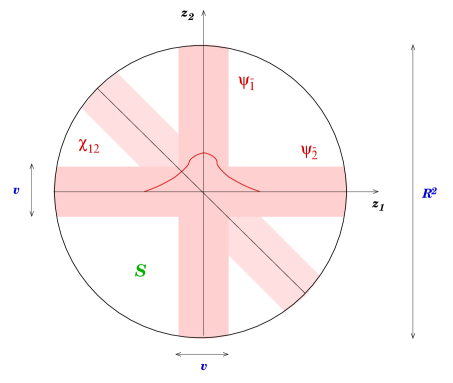
Figure 2: Triple intersection of three matter curves.

4 Yukawa couplings

4.1 Computing Yukawa couplings

We are interested in evaluating the Yukawa coupling of three chiral fields coming from three intersecting matter curves locally described by $z_{1}=0$, $z_{2}=0$ and $z_{1}+z_{2}=0$ in the surface $S$. The piece of the superpotential relevant for Yukawa couplings will be

$$W_{Y}=M_{*}^{4}\int_{S}{\rm Tr\,}({\boldsymbol{A}}\wedge{\boldsymbol{A}}\wedge{\boldsymbol{\Phi}})$$ (4.1)

where $M_{*}$ is the typical mass scale characteristic of the supergravity limit of F-theory. The Yukawa couplings are obtained as overlap integrals over $S$ of the three wave functions involved. In principle such a computation requires a knowledge of the wave functions over the whole complex surface $S$. On the other hand, we know that the wave functions are peaked around the local curves $z_{1}=0$, $z_{2}=0$ and $z_{1}+z_{2}=0$ so that the coupling is dominated by the region around the origin, $z_{1}=z_{2}=0$, where the three curves meet. If this is correct, a local knowledge of the wave functions of the type discussed in the previous sections will be sufficient to evaluate the Yukawa couplings. We will thus be interested on overlap integrals of the form

$$Y=M_{*}^{4}\int_{S}\!d^{2}z_{1}d^{2}z_{2}\,\psi_{\bar{1}}\,\psi_{\bar{2}}\,\varphi_{12}$$ (4.2)

involving zero modes of the curves $z_{1}=0$, $z_{2}=0$, and $z_{1}+z_{2}=0$ respectively, $z_{i}$ being the local coordinates. Given this structure it is natural to assign the physical, e.g. quark/lepton, fields to $\psi_{\bar{\imath}}$ zero modes and $\varphi_{12}$ to the Higgs boson and we will assume this in what follows.

We will then take $\psi_{\bar{1}}$, $\psi_{\bar{2}}$, and $\varphi_{12}$ to be the zero modes localized at the curves $\Sigma_{a}$, $\Sigma_{b}$ and $\Sigma_{c}$ respectively. By supersymmetry the wave function of $\varphi_{12}$ is equal to that of $\chi_{c}$. We have seen in the previous sections that, in the holomorphic gauge, the relevant wave functions in the presence of variable fluxes take the general form

$$\psi_{\bar{1}} = -f(z_{2})e^{-e_{1}m^{2}|z_{1}|^{2}}\,G_{a}(z_{1},{\bar{z}}_{1};q)$$

$$\psi_{\bar{2}} = -g(z_{1})e^{-e_{2}m^{2}|z_{2}|^{2}}\,G_{b}(z_{2},{\bar{z}}_{2};q)$$ (4.3)

$$\varphi_{12} = e^{-\frac{em^{2}}{\sqrt{2}}|z_{1}+z_{2}|^{2}}\,G_{c}(z_{1},{\bar{z}}_{1},z_{2},{\bar{z}}_{2};q,q_{1},q_{2})$$

where $G_{I}$, $I=a,b,c$, are functions which can be computed to any desired order both in fluxes and derivatives of fluxes. Recall that $G_{a}$ and $G_{b}$ depend only on bulk charges whereas $G_{c}$ depends on all charges. In absence of fluxes one simply has $G_{a}=G_{b}=G_{c}=1$. Here $f(z_{2})$ and $g(z_{1})$ are holomorphic functions. As in [19] we will choose a basis in which they are given by $f_{k}=(z_{2}/R)^{3-k}$ and $g_{\ell}=(z_{1}/R)^{3-\ell}$, $k,\ell=1,2,3$, corresponding to the three generations of quarks and leptons. Since there is only one Higgs field we can take the corresponding holomorphic function to be a constant. We then have to perform the integral

$$Y_{k\ell}=M_{*}^{4}\int_{S}\!d^{2}z_{1}d^{2}z_{2}\,e^{-em^{2}(|z_{1}|^{2}+|z_{2}|^{2}+\frac{1}{\sqrt{2}}|z_{1}+z_{2}|^{2})}\,f_{k}(z_{2})\,g_{\ell}(z_{1})\,G(z_{1},{\bar{z}}_{1},z_{2},{\bar{z}}_{2})\ ,$$ (4.4)

where $G=G_{a}G_{b}G_{c}$. To simplify the analysis we have set $e_{1}=e_{2}=e$.

An important point to remark is that turning on fluxes does not induce mixing in the wave functions among different flavors. Indeed, as seen e.g. in eq.(4.3), the flux corrections in $G_{a}$($G_{b}$) do not introduce additional holomorphic dependence on $z_{2}$($z_{1}$) which would signal generation mixing in the wave functions. This is an important simplification because otherwise we would need an additional diagonalization of wave functions in order to extract the physical couplings from eq.(4.2).

The measure in the Yukawa integral can be thought to be

$$d\mu=d^{2}z_{1}d^{2}z_{2}\,e^{-em^{2}(|z_{1}|^{2}+|z_{2}|^{2}+\frac{1}{\sqrt{2}}|z_{1}+z_{2}|^{2})}$$ (4.5)

Clearly, the third exponential, due to the zero mode on $\Sigma_{c}$, breaks the symmetry under separate $U(1)$ rotations $z_{i}\rightarrow e^{i\theta_{i}}z_{i}$. Instead, there is only invariance under the diagonal $U(1)$. This is enough to show that without non-constant fluxes, in which case $G$ cannot depend separately on the antiholomorphic variables, the only non-vanishing Yukawa coupling is $Y_{33}$ because $f_{3}=g_{3}=1$. Thus, the heaviest third generation of quarks and leptons will acquire masses through $Y_{33}$.

As pointed out originally in [19], to generate non-vanishing Yukawa couplings for all families it is necessary to turn on non-constant background fluxes. To see this it is useful to rewrite the measure as

$$d\mu=\frac{1}{4}\,d^{2}u\,d^{2}w\,e^{-em^{2}(\frac{1}{2}|u|^{2}+\frac{1}{2s}|w|^{2})}$$ (4.6)

where $s={\sqrt{2}}-1$. As before, $w=z_{1}+z_{2}$ and $u=z_{1}-z_{2}$. In presence of variable fluxes the function $G$ can furnish adequate powers of $\bar{w}$ and $\bar{u}$ so that the integrand becomes invariant under separate phase rotations of $w$ and $u$. The couplings $Y_{k\ell}$ will thus be non-zero and the light generations will gain masses and mixings. We have introduced the parameter $s$ in order to study also the case $s=1$, which corresponds to ignoring the zero mode exponential from $\Sigma_{c}$. In this situation the measure becomes invariant under separate $U(1)$ rotations $z_{i}\rightarrow e^{i\theta_{i}}z_{i}$ and there will be additional cancellations when computing the integrals.

In performing the integration we will assume that the width of the matter curves is determined by the F-theory scale $M_{*}$, this means $v=1/(em^{2})=1/M_{*}^{2}$. Consistency of the local analysis requires the matter curves to be well localized within $S$. This amounts to the condition $v/R^{2}\ll 1$, which is approximately valid for $v=1/M_{*}^{2}$ because $1/R^{2}=\sqrt{\alpha_{G}}M_{*}^{2}$, and $\sqrt{\alpha_{G}}\simeq 0.2$. In practice we will evaluate the integrals over $S$, with the above measure $d\mu$, by extending $|w|$ and $|u|$ to infinite radius. The main contribution to the integrand still comes from the region near the origin because the measure is sufficiently peaked. The upshot is that in the end all integrals can be done exactly.

Without varying fluxes there is only one non-vanishing Yukawa coupling $Y_{33}$ for the third generation which may be explicitly estimated as

$$Y_{33}^{(0)}=M_{*}^{4}\int_{S}\!d^{2}z_{1}d^{2}z_{2}\,e^{-M_{*}^{2}(|z_{1}|^{2}+|z_{2}|^{2}+\frac{1}{\sqrt{2}}|z_{1}+z_{2}|^{2})}\,=\,\frac{\pi^{2}}{(1+\sqrt{2})}\ .$$ (4.7)

To get the physical Yukawa coupling we really need to work with wave functions normalized to unity, but to actually normalize our wave functions we would need a global knowledge of them over all $S$. We can however make an estimate by neglecting the effect of fluxes and computing the norm of the $\psi_{\bar{\imath}}$ wave functions from

$${\mathcal{C}}\simeq M_{*}^{4}\int_{S}\,e^{-2M_{*}^{2}|z_{i}|^{2}}\,=\,\frac{\pi}{2}M_{*}^{2}R^{2}$$ (4.8)

Thus, the normalized $\psi_{\bar{\imath}}$ wave functions are obtained multiplying our wave functions by the normalization factor ${\mathcal{C}}^{-1/2}$. Similarly computed, the normalization for $\chi_{12}$, arising in the curve $\Sigma_{c}$, is found to be ${\mathcal{C}}^{\prime}={\mathcal{C}}/\sqrt{2}$. We then obtain the normalized third generation Yukawa coupling

$$Y_{33}^{norm}\,\simeq\,\frac{2^{1/4}\pi^{2}}{(1+\sqrt{2})}\left(\frac{2}{\pi M_{*}^{2}R^{2}}\right)^{\!\!\!3/2}\ =\ \frac{2^{7/4}\pi^{1/2}}{(1+\sqrt{2})}\alpha_{G}^{3/4}\ \simeq\ 0.23$$ (4.9)

where we have taken the $SU(5)$ value $\alpha_{G}=1/24$. The $\alpha_{G}^{3/4}$ dependence in eq.(4.9) was previously noted in [16].

The $Y_{33}$ Yukawa just computed is given at the unification scale. Taking into account QCD renormalization effects down to the weak scale there is an extra factor $\simeq 3$ in the case of quarks so that one obtains

$$m_{t}\ \simeq\ 0.23\times 3\times\langle H_{u}\rangle\ =\ 0.69\times 170\ \sin\beta\ \simeq\ 117\ {\rm GeV}$$ (4.10)

where in the last step we have assumed a large value for $\tan\beta=\langle H_{u}/H_{d}\rangle$. This is in reasonable agreement with experiment, given the uncertainties. A large value for $\tan\beta$ is required to understand within this scheme the relative smallness of the masses of b-quark and $\tau$ lepton compared to the top. For them one finds

$$m_{b}\ \simeq\ \frac{m_{t}}{\tan\beta}\ \quad;\quad m_{\tau}\ \simeq\ \frac{m_{t}}{3\tan\beta}$$ (4.11)

which gives reasonable agreement for $\tan\beta\simeq 35-45$. Note that the tau lepton is lighter by a factor $\simeq 3$ due to the absence of QCD renormalization.

There are also subleading contributions to $Y_{33}$ from flux corrections which appear even for constant flux (see appendix B.1). We will eventually neglect all subleading corrections so for consistency we will only keep the leading term in $Y_{33}$. When we calculate the rest of the Yukawa couplings we will then normalize them relative to the 3rd generation Yukawa in eq.(4.7).

4.2 The case of a constant $\chi_{c}$ wave function

We study first this simple case because it has some interesting features by itself. Furthermore, a constant wave function is unlocalized and hence could serve to give an idea of the results to be expected for Yukawa couplings in which the third particle, presumably the Higgs field, lives in the bulk rather than in a localized matter curve. Such type of couplings do appear in type IIB and F-theory models in which the base $S$ is not del Pezzo.

When $\chi_{c}$ is a constant, taken equal to one, the Yukawa couplings are determined by

$$Y_{k\ell}\left|{}_{\chi_{c}=1}\right.=M_{*}^{4}\int_{S}\!d^{2}z_{1}d^{2}z_{2}\,e^{-em^{2}(|z_{1}|^{2}+|z_{2}|^{2})}\,f_{k}(z_{2})\,g_{\ell}(z_{1})\,G_{a}(z_{1},{\bar{z}}_{1};q)G_{b}(z_{2},{\bar{z}}_{2};q)$$ (4.12)

where $q$ denotes the bulk charges. Substituting the expressions for $G_{a}$ and $G_{b}$, which may be extracted from the wave functions in appendix A.2, leads to

$$Y_{k\ell}\left|{}_{\chi_{c}=1}\right.\ =\ \pi^{2}\,\delta_{k-3,\ell-3}$$ (4.13)

Hence, the flux-induced distortion of the wave functions does not give rise to any new couplings, only the coupling $Y_{33}$ which is there already for constant fluxes is non-vanishing. This is true for any order in the flux expansion. In the next section and in appendix B we will provide some examples of the cancellation in the expansion of the $Y_{k\ell}$. The result can also be proven analytically. In fact, notice that in (4.12) the integrals in $z_{1}$ and $z_{2}$ decouple so that it suffices to show that $I_{\ell}=\int\!d^{2}z_{1}e^{-em^{2}|z_{1}|^{2}}z_{1}^{3-\ell}G_{a}$ vanishes when $\ell=1,2$. The key point is that $e^{-em^{2}|z_{1}|^{2}}G_{a}$ can be written as $\frac{1}{z_{1}}\bar{\partial}_{\bar{1}}F_{a}$, as explained in appendix A.2. The function $F_{a}$ can be extracted explicitly, in particular it goes to zero when $|z_{1}|\to\infty$ and to 1 when $|z_{1}|\to 0$. It is then easy to show that $I_{\ell}=0$ for $\ell=1,2$.

The main conclusion is that in order to get non-trivial fermion mass hierarchies one needs all three wave functions to be localized on matter curves. We then proceed to this most interesting case of three overlapping localized wave functions.

4.3 Yukawa matrices

The physical Yukawas are obtained evaluating the overlapping integral in eq.(4.4) which is dominated by the region close to the intersection point. The heavy task is to compute the function $G$ by substituting the wave functions found in the previous sections expanded in powers both of the flux and derivatives of the flux. In the end each Yukawa coupling reduces to a sum of Gaussian integrals that can evaluated analytically. As expected, $Y_{ij}$ and $Y_{ji}$ are related by an appropriate exchange of flux parameters.

To begin we have considered the simplest case in which the field strengths are expanded only to linear order. This means that we only take into account the first derivative of the fluxes (i.e. the $\alpha_{I}$ and $\delta$ parameters) and neglect the effect of higher derivatives. The integrals can be determined exactly. For example, the coupling $Y_{23}$ is found to be

$$Y_{23}=\frac{v^{2}}{3R}\big{[}\,(s-1)^{2}\bar{\alpha}_{a}+(s^{2}-1)\bar{\alpha}_{b}-3s\bar{\alpha}_{c}+s(2s+3)\bar{\delta}\,\big{]}$$ (4.14)

where $s=\sqrt{2}-1$ is the parameter appearing in the measure (4.6). This coupling is normalized with respect to $Y_{33}^{(0)}=\pi^{2}s$. This exact expression also shows that when $s=1$ the terms that depend purely on $\alpha_{a}$ and $\alpha_{b}$ completely drop out. In all couplings it happens that for $s=1$ all pieces involving only parameters of the curves $\Sigma_{a}$ and $\Sigma_{b}$ do cancel out. This implies that when $\chi_{c}=1$, the only coupling that survives is $Y_{33}$.

In appendix B.1 we display the leading terms in the expansion in $\alpha$-fluxes for each entry of the Yukawa matrix, normalized with respect to $Y_{33}^{(0)}$. Some of the elements $Y_{ij}$ have complicated expressions in terms of the flux parameters but the pattern behind can be easily understood. Schematically, the couplings turn out to be

$$Y_{ij}\sim\left(\frac{v^{2}\bar{\alpha}}{R}\right)^{3-i}\left(\frac{v^{2}\bar{\alpha}}{R}\right)^{3-j}$$ (4.15)

As explained in section 3.4, we have for instance $\alpha_{a}=2\pi\sqrt{\alpha_{G}}q_{a}\tilde{\alpha}_{1B}M_{*}^{2}/R$. Therefore, we find $v^{2}\alpha_{a}/R=2\pi\alpha_{G}q_{a}\tilde{\alpha}_{1B}$, because $v=1/M_{*}^{2}$ and $M_{*}^{2}R^{2}=1/\sqrt{\alpha_{G}}$.

More generally, the corrections to the Yukawa couplings due to first derivatives of the fluxes have the general form

$$Y_{ij}\ \simeq\ \xi_{ij}\,\left(2\pi\alpha_{G}(aq+a^{\prime}q^{\prime})\right)^{(3-i)}\left(2\pi\alpha_{G}(aq+a^{\prime}q^{\prime})\right)^{(3-j)}$$ (4.16)

Here we have simply replaced the $\tilde{\alpha}_{iB}$ and the $\tilde{\alpha}_{i}^{(j)}$ of section 3.4 by generic constants $a$ and $a^{\prime}$ in order to get an idea of the structure. The $\xi_{ij}$ are numerical coefficients appearing upon integration which are typically in the range $0.1-10$, as may be seen in appendix B.1. The constants $q$ and $q^{\prime}$ are the bulk and matter curve $U(1)$ charges respectively. Recall that for the fields in matter curves $\Sigma_{a}$ and $\Sigma_{b}$, which include quarks and leptons, one has $q^{\prime}=0$ and the corresponding $\alpha_{a}$ and $\alpha_{b}$ parameters only depend on the bulk $U(1)$ charges. This is not the case for the matter curve $\Sigma_{c}$, the parameters $\alpha_{c}$ and $\delta$ do depend on the matter curve charges. Note that the normalization of the $U(1)$ charges is relevant here. As we explained, for the $SU(5)$ case for integer hypercharge there is a normalization factor $1/\sqrt{60}$ and the $U(1)$’s on the matter curves containing $10$’s and ${\bar{5}}$’s have normalization $1/\sqrt{40}$ and $1/\sqrt{60}$ respectively.

We have just discussed the general form of each of the terms in the Yukawa couplings shown in appendix B.1. To get more accurate results we would need to specify the different flux parameters for the three matter curves involved. In particular, we would need a precise knowledge of how the $U(1)$ field strengths vary in the vicinity of the intersecting points. In principle, given a set of assumptions about the derivatives of fluxes on the different matter curves in a concrete model, the formulas in appendix B will allow us to compute the different Yukawa couplings.

It is already quite encouraging that a hierarchical structure of fermion masses seems to be built in. Using eq.(4.16) we can further estimate the Yukawa couplings by taking into account the normalization of the $U(1)$ charges explained in section 3.4. To this end we will write the bulk charges as $q=\hat{q}e_{B}$, where $\hat{q}$ is an integer and $e_{B}$ is the bulk charge normalization. We will similarly write $q^{\prime}=\hat{q}^{\prime}e$, where $e$ is the normalization of the appropriate $U(1)$ on the matter curve, and reabsorb the ratio $e/e_{B}$ into the coefficient $a^{\prime}$. It is also convenient to introduce $\alpha_{U(1)}=e_{B}^{2}\alpha_{G}$, which corresponds to the $U(1)$ fine structure constant normalized for integer charges of massless fields. We then conclude that the Yukawa matrix has the form

$$Y^{(1)}\ \sim\ \left(\begin{array}[]{ccc}\epsilon^{4}\eta^{4}&\epsilon^{3}\eta^{3}&\epsilon^{2}\eta^{2}\\ \epsilon^{3}\eta^{3}&\epsilon^{2}\eta^{2}&\epsilon\eta\\ \epsilon^{2}\eta^{2}&\epsilon\eta&1\end{array}\right)\quad;\quad\epsilon=2\pi\sqrt{\alpha_{U(1)}}\quad;\quad\eta=\sqrt{\alpha_{G}}$$ (4.17)

In the terminology of [19], we can say that the physical parameter $\epsilon$, which is tied to the $\alpha_{I}$ coefficients, controls the flux expansion. The parameter $\eta$ is related to powers of the width $v$ and the overall radius $R$ that appear in the couplings and controls instead the derivative expansion. Taking $\alpha_{G}=1/24$ and $e_{B}=e_{Y}=1/\sqrt{60}$ gives $\epsilon=0.16$, $\eta=0.20$ so that $\epsilon\eta\simeq 1/31$. We then find

$$Y_{ij}\ \simeq\ \xi_{ij}\,\left(\frac{a\hat{q}+a^{\prime}\hat{q}^{\prime}}{31}\right)^{(3-i)}\left(\frac{a\hat{q}+a^{\prime}\hat{q}^{\prime}}{31}\right)^{(3-j)}$$ (4.18)

Therefore, the fermion hierarchies are roughly of the type

$$(m_{3}:m_{2}:m_{1})\ \simeq\ (1:10^{-3}(a\hat{q}+a^{\prime}\hat{q}^{\prime})^{2}:10^{-6}(a\hat{q}+a^{\prime}\hat{q}^{\prime})^{4})$$ (4.19)

in qualitative agreement with the observed spectra of quarks and leptons. In the next chapter we discuss in slightly more detail to what extent this structure may be successful in describing the pattern of quark and lepton masses.

Let us now see what happens if further terms in the derivative expansion of the fluxes were non-negligible. In particular, we have studied the corrections to the Yukawa couplings when the second derivative flux parameters $\beta_{I}$ and $\rho$ are non-zero. We found that the couplings $Y_{13}$ and $Y_{22}$ receive leading contributions linear in $\beta_{I}$ or $\rho$. They also have quadratic corrections, proportional to the constant coefficients ${\mathcal{M}}$ and ${\mathcal{N}}$ of the various curves times the $\beta_{I}$ or $\rho$, that are subleading and can be neglected. The leading linear terms are

$$Y_{13} \!=\! \frac{v^{3}}{8R^{2}}\big{[}\,3(s-1)^{3}\bar{\beta}_{a}+3(s+1)(s^{2}-1)\bar{\beta}_{b}-16s^{2}\bar{\beta}_{c}+2s(3s^{2}+8s+6)\bar{\rho}\,\big{]}$$ (4.20)

$$Y_{22} \!=\! \frac{v^{3}}{8R^{2}}\big{[}\,3(s-1)(s^{2}-1)(\bar{\beta}_{a}+\bar{\beta}_{b})+2s(s^{2}-2)\bar{\rho}\,\big{]}$$ (4.21)

where $s=\sqrt{2}-1$ as before. Here we notice again that when $\chi_{c}=1$ the couplings will vanish identically because in this case $s=1$ while $\beta_{c}=0$ and $\rho=0$. The couplings $Y_{12}$ and $Y_{11}$ have leading corrections typically proportional to $\alpha_{I}\beta_{J}$ and $\beta_{I}\beta_{J}$ respectively, but the exact expressions are too long to display. In appendix B.2 we show the numeric results for the extra leading contributions

To figure out the size of the corrections due to the second derivative flux parameters we will estimate them for the case of the $Y_{11}$ and $Y_{22}$ Yukawa couplings. We have

$$Y_{22} \ \sim\ \frac{v^{3}\bar{\beta}}{R^{2}}\simeq\ \ \frac{2\pi v^{3}\sqrt{\alpha_{U(1)}}(b\hat{q}+b^{\prime}\hat{q}^{\prime})M_{*}^{2}}{R^{4}}=2\pi\sqrt{\alpha_{U(1)}}\alpha_{G}(b\hat{q}+b^{\prime}\hat{q}^{\prime})$$ (4.22)

$$Y_{11} \ \sim\ \frac{v^{6}\bar{\beta}^{2}}{R^{4}}\simeq\ \ \frac{(2\pi)^{2}v^{6}\alpha_{U(1)}(b\hat{q}+b^{\prime}\hat{q}^{\prime})^{2}M_{*}^{4}}{R^{8}}=(2\pi)^{2}\alpha_{G}^{2}\alpha_{U(1)}(b\hat{q}+b^{\prime}\hat{q}^{\prime})^{2}$$ (4.23)

These terms would contribute to the hierarchy of fermion masses as

$$(m_{3}:m_{2}:m_{1})\ \simeq\ (1:(2\pi)\alpha_{G}\sqrt{\alpha_{U(1)}}:(2\pi)^{2}\alpha_{G}^{2}\alpha_{U(1)})\ .$$ (4.24)

We can evaluate the remaining couplings in the same way (the first order in fluxes $Y_{23}$ and $Y_{32}$ as well). Including the zeroth order $Y_{33}$ we obtain the structure

$$Y^{(2)}\ \sim\ \left(\begin{array}[]{ccc}\epsilon^{2}\eta^{4}&\epsilon^{2}\eta^{3}&\epsilon\eta^{2}\\ \epsilon^{2}\eta^{3}&\epsilon\eta^{2}&\epsilon\eta\\ \epsilon\eta^{2}&\epsilon\eta&1\end{array}\right)$$ (4.25)

Since $\epsilon\simeq\eta$, there are hierarchies $(1:\epsilon^{3}(b\hat{q}+b^{\prime}\hat{q}^{\prime}):\epsilon^{6}(b\hat{q}+b^{\prime}\hat{q}^{\prime})^{2})$. We see that for coefficients of order one, these corrections will generically dominate over the corresponding terms in the flux expansion with only first derivatives of fluxes.

We can go one step beyond and consider also the effect of terms of order three and four in the derivative expansion of the fluxes. In this case, to leading order there appear contributions to $Y_{12}$, $Y_{21}$ and $Y_{11}$. The results are given in B.3 where we also explain the notation. The additional corrections may be approximated by

$$Y_{11} \sim \frac{v^{5}\bar{D}}{R^{4}}\simeq\frac{2\pi v^{5}\sqrt{\alpha_{U(1)}}(d\hat{q}+d^{\prime}\hat{q}^{\prime})M_{*}^{2}}{R^{8}}=2\pi\sqrt{\alpha_{U(1)}}\alpha_{G}^{2}(d\hat{q}+d^{\prime}\hat{q}^{\prime})$$ (4.26)

$$Y_{12} \sim Y_{21}\sim\frac{v^{4}\bar{C}}{R^{3}}=\frac{2\pi v^{4}\sqrt{\alpha_{U(1)}}(c\hat{q}+c^{\prime}\hat{q}^{\prime})M_{*}^{2}}{R^{6}}=2\pi\sqrt{\alpha_{U(1)}}\alpha_{G}^{3/2}(c\hat{q}+c^{\prime}\hat{q}^{\prime})$$ (4.27)

In this case there are new contributions to the Yukawa couplings of the form

$$Y^{(3,4)}\ \sim\ \left(\begin{array}[]{ccc}\epsilon\eta^{4}&\epsilon\eta^{3}&0\\ \epsilon\eta^{3}&0&0\\ 0&0&0\end{array}\right)$$ (4.28)

Thus, the first generation Yukawa has corrections of order $Y_{11}\simeq\epsilon\eta^{4}$.

The contributions leading to the terms captured by $Y^{(1)}$ are an explicit evaluation of the flux expansion of the authors of [19]. On the other hand, their derivative expansion would correspond to taking the terms linear in $\epsilon$ in $Y^{(1)}$, $Y^{(2)}$ and $Y^{(3,4)}$ above. Thus, this derivative expansion has the structure

$$Y^{DER}\ \sim\ \left(\begin{array}[]{ccc}\epsilon\eta^{4}&\epsilon\eta^{3}&\epsilon\eta^{2}\\ \epsilon\eta^{3}&\epsilon\eta^{2}&\epsilon\eta\\ \epsilon\eta^{2}&\epsilon\eta&1\end{array}\right)$$ (4.29)

Note however that, for instance in $Y^{(2)}$, we also find corrections which do not correspond to either of both expansions.

As a general conclusion, one observes that, for a given Yukawa matrix element, the correction due to a higher order term in the derivative expansion will always dominate over the flux expansion.

5 Fermion Yukawa couplings in F-theory GUT’s

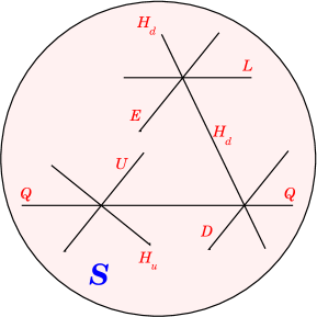
Figure 3: Intersecting matter curves and Yukawa couplings.

In the previous sections we have studied the zero modes of the 8-dimensional quasi-topological field theory as well as the computation of the Yukawa couplings using these zero modes, without specifying any particular geometry nor identifying the nature of the three particles involved in the couplings. We did neither specify the bulk $U(1)$ to be considered, which could be hypercharge in $SU(5)$, $B$-$L$ or other in $SO(10)$. In a GUT model, the quark, lepton and Higgs superfields will be localized in matter curves like those we have described (see figure 3). We will have Yukawa couplings from a superpotential of the form

$$W_{Yuk}\ =\ Y^{U}_{ij}Q^{i}U^{j}H_{u}\ +\ Y^{D}_{ij}Q^{i}D^{j}H_{d}\ +\ Y^{L}_{ij}L^{i}E^{j}H_{d}$$ (5.1)

in an obvious notation. In principle the intersection points of the different matter curves will be different and, correspondingly the flux parameters $\alpha_{I}$, $\beta_{I}$, etc., will also be different at each intersection. The geometry of each given model may constrain the possibilities though. For example, in an $SU(5)$ GUT the left-handed leptons $L^{i}$ and the right-handed $D$-quarks $D^{j}$ live in the same matter curve. In other settings that need not be the case. For example, in a flipped SU(5) setting, $D$, $U$ and $L$ masses come from independent couplings $10\times 10\times 5_{H}$, $10\times{\bar{5}}\times{\bar{5}}_{H}$ and $1\times{\bar{5}}\times{5}_{H}$.

Another point to emphasize is that in previous chapters we have made use of the possibility of choosing a local basis of holomorphic wave functions of the canonical form $1,z_{i},z_{i}^{2}$ at the intersection point. Note however that in the case of quarks we cannot make use of the freedom to choose that basis both at the intersection point leading to $U$-quark masses and that giving rise to $D$-quark masses. On the other hand, if the holomorphic basis at both points are very different, one expects very large CKM mixing angles. This may be an indication that both points must be quite close in $S$ in order for the basis to be aligned to give reduced mixing, as required phenomenologically [19]. That points towards further unification into at least $E_{7}$ at the F-theory level.

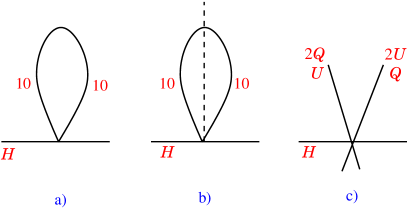
Figure 4: Matter curves intersecting to provide $U$-quark Yukawas.

An important issue in F-theory grand unification is the generation of appropriate Yukawa couplings for the $U$-quarks. After all, one of the main motivations for going to F-theory GUT’s instead of perturbative IIB orientifolds is that in the former case these couplings are allowed, while they are perturbatively forbidden in type IIB orientifolds. In $SU(5)$ the $U$-quark Yukawas come from couplings $10^{i}\times 10^{j}\times 5_{H}$, and if such coupling comes from three distinct matter curves, there can be no diagonal $U$-quark couplings. This implies that the trace of $Y^{U}$ vanishes which makes impossible a hierarchy of $U$-quark masses. In [15, 16, 19] it was suggested that the matter curve associated to the $10$’s in $SU(5)$ could self-pinch as in figure 4-a, allowing for diagonal entries. It was noted though [33] that in such configuration the two branches of the wave functions of the $10$ are independent so that there would be two independent rank one contributions to $Y^{U}$. This would then lead to a rank two Yukawa matrix, with no automatic hierarchical structure. In [33] (see also [19]) it was suggested that in fact the two independent branches of the wave functions could be identified by some symmetry in the geometry (figure 4-b). In such a case the two rank one contributions would be identical and rank one (before the addition of flux effects). It was also argued that these symmetries are ubiquitous in F-theory and correspond to non-trivial monodromies. Another alternative in order to obtain diagonal entries in $U$-quark Yukawa couplings was also suggested in [20]. It is more easily described in $SO(10)$ but it also applies to $SU(5)$. In the context of $SO(10)$ the Yukawa couplings come from terms $16^{i}\times 16^{j}\times 10_{H}$. If one associates both $16$’s in the coupling to two matter curves $\Sigma_{a}$ and $\Sigma_{b}$, and one allows for appropriate $B$-$L$ flux with opposite restriction on the curves, the massless spectrum splits as in figure 4-c. One curve has matter content $2Q+U$, and the other $2U+Q$, and this splitting allows for diagonal couplings. In fact, as already noted in [20], both matter curves could be local branches of some self-pinched matter curve, as in figures 4-a and 4-b. An interesting feature of this possibility is that the mixing of the first generation with the other two is expected to be suppressed. In what follows we will not specify the particular scheme for the understanding of the $U$-quark Yukawa couplings. We will just consider that the approximate rank one structure already assumed in the previous sections does apply.

In this section we make a preliminary analysis of the application of our previous results to the description of quark and lepton spectra. We would like to see to what extent flux distortion may explain the data. Let us first consider for definiteness the case of a $SU(5)$ GUT broken down to the SM by fluxes along the hypercharge direction. Let us first see whether the flux-induced distortion of wave functions due to first derivatives of fluxes is enough to describe the observed structure of quarks and leptons. In order to get manageable results we will first assume for simplicity that the fluxes going through the third matter curve are approximately constant, i.e. $\alpha_{c}=\beta_{c}=\delta=\rho=0$ (we will also denote the subscripts $(a,b)$ as $(1,2)$ hereafter). Under these circumstances the formulas in appendix B.1 substantially simplify. In particular, the diagonal entries reduce to

$$Y_{22} \simeq \epsilon^{2}\eta^{2}\left(0.067(Y_{R}^{2}{\bar{a}}_{1}^{2}+Y_{L}^{2}{\bar{a}}_{2}^{2})+0.11\ Y_{R}Y_{L}{\bar{a}}_{1}{\bar{a}}_{2}\right)$$ (5.2)

$$Y_{11} \simeq \epsilon^{4}\eta^{4}\left(0.10(Y_{R}^{4}{\bar{a}}_{1}^{4}+Y_{L}^{4}{\bar{a}}_{2}^{4})+0.09Y_{R}Y_{L}{\bar{a}}_{1}{\bar{a}}_{2}(Y_{R}^{2}{\bar{a}}_{1}^{2}+Y_{L}^{2}{\bar{a}}_{2}^{2})+0.12Y_{L}^{2}Y_{R}^{2}{\bar{a}}_{1}^{2}{\bar{a}}_{2}^{2}\right)$$

where $Y_{R},Y_{L}$ are the (integer) hypercharges of right-handed fermions (on matter curve $\Sigma_{a}$) and left-handed ones (on matter curve $\Sigma_{b}$). Recall that

$$\epsilon\ =\ 2\pi\sqrt{\alpha_{Y}}\ =\frac{2\pi}{\sqrt{60}}\sqrt{\alpha_{G}}\ \simeq\ 0.16\quad;\quad\eta\ =\ \sqrt{\alpha_{G}}\ \simeq\ 0.20$$ (5.3)

where we have taken into account the hypercharge normalization factor $e_{Y}=1/\sqrt{60}$. Note that, as we mentioned before, the wave functions in matter curves $\Sigma_{a}$ and $\Sigma_{b}$ in the holomorphic gauge have no dependence on the $U(1)_{i}$ fluxes, they only depend on the bulk fluxes which go in this case along hypercharge. Here $a_{1,2}$ are the adimensional constants parametrizing the variation of the bulk flux close to the intersection point. Note that in principle these parameters may be different for the three different Yukawa couplings, i.e. there are $a^{U,D,L}_{1,2}$. To get an idea of the size of the Yukawas let us for the moment assume that $a^{U.D,L}_{1}\simeq a^{U,D,L}_{2}\simeq a^{U,D,L}$. Note that in this case that we neglect the flux variation for the Higgs matter curve, the Yukawa matrix is strongly dependent on the hypercharge of the quarks and leptons involved in the couplings. Since the maximum value of the quark and lepton hypercharges is $|Y_{max}|=6,4,2$ respectively for leptons and $U$ and $D$-quarks, one expects larger effects for leptons, $U$-quarks and $D$-quarks in that order.

Inserting the values of the hypercharges for the different particles involved in each Yukawa coupling leads to the results in table 2 for the diagonal Yukawas.

Yukawa	$Y_{33}$	$Y_{22}$	$Y_{11}$
$Y^{U}$	1	$0.7(a^{U})^{2}\times 10^{-3}$	$2.2(a^{U})^{4}\times 10^{-5}$
$Y^{U}$(exp)	1	$(3-4)\times 10^{-3}$	$(0.5-1.6)\times 10^{-5}$
$Y^{L}$	1	$1.1(a^{L})^{2}\times 10^{-3}$	$1.1(a^{L})^{4}\times 10^{-4}$
$Y^{L}$(exp)	1	$5.9\times 10^{-2}$	$2.8\times 10^{-4}$
$Y^{D}$	1	$0.6(a^{D})^{2}\times 10^{-3}$	$3.2(a^{D})^{4}\times 10^{-6}$
$Y^{D}$ (exp)	1	$(1-3)\times 10^{-2}$	$(0.6-1.8)\times 10^{-3}$

Table 2: Hierarchies of fermion masses from the flux expansion. First order in derivatives.

The couplings are normalized to the one of the corresponding third generation particle. We also show for comparison experimental results for that hierarchy evaluated at the electroweak scale from [46]. The results for the $U$-quarks hierarchies are encouraging, for values $a^{U},a^{L}\simeq 1$ one can describe reasonably well the observed pattern. For the case of charged leptons the mass of the electron is again well described for $a^{L}\simeq 1$. However, the mass of the muon would turn out too light unless $a^{L}\simeq 7.3$, which would be quite large and incompatible with the $a^{L}\simeq 1$ required for the electron. Thus, the correct numerical description would require some further contribution for the muon. Alternatively, it could be that for charged leptons neglecting the flux variation coming from the Higgs matter curve is not the correct assumption. For the case of the the $D$-quark hierarchies one would need slightly large values $a^{D}\simeq 5.8$ and $a^{D}\simeq 4$ for $Y_{22}$ and $Y_{11}$ respectively.

Let us now explore what would be the effect of higher order terms in the derivatives of the fluxes. If we consider second order in derivatives there are extra corrections which may be extracted from appendix B.2. We will again set to zero all flux parameters from the curve $\Sigma_{c}$. The corresponding diagonal terms are found to be

$$Y_{22} \simeq \epsilon\eta^{2}\ 0.18\left(Y_{R}{\bar{b}}_{1}+Y_{L}{\bar{b}}_{2}\right)$$ (5.4)

$$Y_{11} \simeq \epsilon^{2}\eta^{4}\ (-0.23(Y_{R}^{2}{\bar{b}}_{1}^{2}+Y_{L}^{2}{\bar{b}}_{2}^{2})+0.29Y_{L}Y_{R}{\bar{b}}_{1}{\bar{b}}_{2})$$

Again taking $b^{U,D,L}_{1}\simeq b^{U,D,L}_{2}\simeq b^{U,D,L}$ yields contributions as in table 3.

Yukawa	$Y_{33}$	$Y_{22}$	$Y_{11}$
$Y^{U}$	1	$3.4(b^{U})\times 10^{-3}$	$2.1(b^{U})^{2}\times 10^{-4}$
$Y^{L}$	1	$3.4(b^{L})\times 10^{-3}$	$6.4(b^{L})^{2}\times 10^{-4}$
$Y^{D}$	1	$3.4(b^{D})\times 10^{-3}$	$2.3(b^{D})^{2}\times 10^{-5}$

Table 3: Hierarchies of fermion masses from the flux expansion. Second order in derivatives.

Note that here the $Y_{22}$ entries have the same structure because in the three cases $Y_{R}+Y_{L}=\pm 3$ (we are ignoring the overall sign of the contribution which is not relevant for this estimate). As expected, the corrections to the Yukawa couplings are always higher than those coming from only first derivatives. This is true even for the leptons, which have the highest maximal hypercharge and hence get the largest contribution to first order in derivatives. In fact, to avoid too large $Y_{11}^{U,L}$ values one rather needs $b^{U},b^{L}<1$. On the other hand, the contribution to $Y_{22}^{L}$ is still too small. The same happens with the $D$-quarks, one would need $b^{D}\simeq 5.6$ to reproduce the observed $D$-quark mass hierarchies, so that strong variation is again required for $D$-quarks. Terms of order 3 and 4 in flux derivatives could also add to the relatively large values of the $D$-quarks. Equation (4.26) shows that the expected contribution is of order $Y_{11}\simeq\epsilon\eta^{4}(d\hat{q}+d^{\prime}\hat{q}^{\prime})\simeq 2.6d\times 10^{-4}$, which reproduces the $D$-quark mass result for a flux parameter $d\simeq 2.4$. Hence, if we do not want to rely on relatively large flux parameters the case of $D$-quarks requires substantial input from higher orders in the derivative expansion, up to order four.

In [19] it was pointed out that the flux expansion to first order in derivatives gives a good explanation of the hierarchies observed for leptons and $U$-quarks but terms coming from the higher derivative flux expansion were needed in order to describe the hierarchies for $D$-quarks. It was also suggested that a possible reason for this different behavior could arise from the fact that leptons and $U$-quarks have higher maximal hypercharge than the $D$-quarks. We indeed find that the hierarchies for $U$-quarks may be quite well described by first order flux variations of order one. The resulting electron mass is also of the correct order. However, the dependence on hypercharge does not seem to explain the different behavior of $L$ and $U$ compared to $D$ fermions. In particular, higher derivative terms always generically dominate over the first order terms, even taking into account the hypercharge dependence. The milder behavior of the $D$-quark hierarchies can be understood either by assuming a relatively strong first/second order flux variation (i.e. $a^{D}\simeq 5.8$ or $b^{D}\simeq 5.6$) or larger 4th order contributions with $d\simeq 2.4$. The muon has the tendency to come out too light which may indicate that neglecting flux variation in the Higgs matter curve could perhaps be inappropriate for the leptons and possibly for the $D$-quark matter curves.

If we assume that $U$-quarks get their Yukawas already at first order in derivatives (eq.(4.17)) and on the contrary the $D$-quarks need a dominant contribution at order two or higher (eq.(4.25) or eq.(4.29), it does not matter for this approximation), we can also give an estimate of the CKM mixing matrix [19]. Indeed in this case the respective mass squared matrices will be proportional to

$$Y^{U}(Y^{U})^{\dagger}\ \sim\ \left(\begin{array}[]{ccc}\epsilon^{4}\eta^{4}&\epsilon^{3}\eta^{3}&\epsilon^{2}\eta^{2}\\ \epsilon^{3}\eta^{3}&\epsilon^{2}\eta^{2}&\epsilon\eta\\ \epsilon^{2}\eta^{2}&\epsilon\eta&1\end{array}\right)\ ;\ Y^{D}(Y^{D})^{\dagger}\ \sim\ \left(\begin{array}[]{ccc}\epsilon^{2}\eta^{4}&\epsilon^{2}\eta^{3}&\epsilon\eta^{2}\\ \epsilon^{2}\eta^{3}&\epsilon^{2}\eta^{2}&\epsilon\eta\\ \epsilon\eta^{2}&\epsilon\eta&1\end{array}\right)$$ (5.5)

Then, as in [47], one can estimate the matrices $V^{U,D}$ which diagonalize each of them

$$V^{U}\ \sim\ \left(\begin{array}[]{ccc}1&\epsilon\eta&\epsilon^{2}\eta^{2}\\ \epsilon\eta&1&\epsilon\eta\\ \epsilon^{2}\eta^{2}&\epsilon\eta&1\end{array}\right)\ ;\ V^{D}\ \sim\ \left(\begin{array}[]{ccc}1&\eta&\epsilon\eta^{2}\\ \eta&1&\epsilon\eta\\ \epsilon\eta^{2}&\epsilon\eta&1\end{array}\right)$$ (5.6)

The CKM matrix, $V^{CKM}\simeq V^{U}(V^{D})^{\dagger}$, then turns out to be

$$V^{CKM} \simeq \left(\begin{array}[]{ccc}1&\eta&\epsilon\eta^{2}\\ \eta&1&\epsilon\eta\\ \epsilon\eta^{2}&\epsilon\eta&1\end{array}\right)\ \simeq\ \left(\begin{array}[]{ccc}1&\alpha_{G}^{1/2}&2\pi\alpha_{Y}^{1/2}\alpha_{G}\\ \alpha_{G}^{1/2}&1&2\pi\alpha_{Y}^{1/2}\alpha_{G}^{1/2}\\ 2\pi\alpha_{Y}^{1/2}\alpha_{G}&2\pi\alpha_{Y}^{1/2}\alpha_{G}^{1/2}&1\end{array}\right)$$ (5.13)

$$\simeq \left(\begin{array}[]{ccc}1&0.20&0.006\\ 0.20&1&0.03\\ 0.006&0.03&1\end{array}\right)$$ (5.17)

which is in reasonable agreement with experiment. This structure is similar to that found in [19], although in comparison, in the above formula the separate dependence on the hypercharge flux is explicit and the 3rd generation mixing is slightly smaller.

As a general conclusion, in this simplified scheme in which we have set the flux variation in the third curve to zero, one can reproduce the general pattern of quark and lepton hierarchies as well as quark mixing, for reasonable choices of flux variation parameters. This is particularly the case for the $U$-quarks and the electron. Nevertheless, a more complete numerical study, not neglecting flux parameters of the Higgs matter curve, may be required to get full agreement. The order of magnitude estimates for the CKM matrix are on the other hand quite promising. We leave a more detailed phenomenological analysis of this framework for future work.

6 Final comments

In this paper we have studied the local structure of zero mode wave functions of chiral matter fields in F-theory compactifications. We have solved the relevant differential equations for the zero modes which were derived from local Higgssing in the world-volume effective action of the F-theory 7-branes [15]. These wave functions have a Gaussian profile centered on the matter curves and become distorted in the presence of $U(1)$ fluxes both on the bulk and on the matter curves themselves. In our approach we first write the fluxes in a power series of the local coordinates and then make a perturbative expansion of the wave functions in powers of the flux coefficients. In this way we obtain expressions which may then be applied to compute physical quantities of interest. In this paper we have concentrated on the calculation of Yukawa couplings but the wave functions could also help to examine other problems. For instance, they could be used to explore the effects of closed string fluxes and warping on the effective action, which could prove important in relation to compactifications with broken supersymmetry.

With the wave functions at our disposal we have computed Yukawa couplings by performing explicitly the overlap integrals of the three wave functions linked to fermions and the Higgs field. By choosing an appropriate gauge, the wave functions of quark or lepton generations are shown to depend only on the bulk fluxes but not on the extra $U(1)$’s associated to the unfolding of the singularities. For example, in the case of a $SU(5)$ F-theory GUT broken to the SM by hypercharge flux, the effective distortion of the wave function depends on the hypercharge of the specific particle considered. The Yukawa integrals can be done analytically and in appendix B we provide the leading terms in the flux expansion. One interesting fact we find is that for a constant non-localized Higgs wave function, presumably corresponding to a Higgs field living on the bulk of the base $S$, the flux distortion cancels in such a way that the possible Yukawa matrices remain of rank one. On the other hand, when the three wave functions are localized, corresponding to three intersecting matter curves, a non-constant $U(1)$ flux gives rise naturally to a hierarchy of Yukawa couplings as first pointed out in [19].

We have applied our findings to the understanding of the observed hierarchies of quark and lepton masses and mixings. In a simplified situation in which the flux variation in the Higgs matter curve is negligible we obtain explicit compact formulas for Yukawa couplings as a function of flux parameters and the charges of the bulk $U(1)$. In a $SU(5)$ setting broken to the SM by hypercharge flux, the resulting Yukawa couplings depend on different powers of the hypercharge of each quark and lepton. It turns out that reasonable values of flux parameters, involving only a first derivative expansion of the fluxes, can account for the hierarchical structure of the masses of $U$-quarks and the electron. The explanation of $D$-quark hierarchies seems to require larger contributions from the higher order terms in the flux derivative expansion. A reasonable semiquantitative understanding of the CKM matrix is then obtained somewhat analogous to the results in [19].

The natural appearance of hierarchies for masses and mixings looks quite promising. However, a full explanation of the data would require a more detailed phenomenological analysis. In particular in the numerical estimations we assumed weakly varying fluxes in the Higgs matter curve, which needs not necessarily be the case. Furthermore, we also took flux variations of the same order for the matter curves corresponding to left- and right-handed fermions, which again is suggestive but not generally true. We think that our explicit formulas are a good starting point for a more thorough investigation which we plan to carry out elsewhere [48].

Another interesting topic to address is the origin and structure of neutrino masses, which seem to follow a pattern quite distinct from that of quarks. Here the crucial point is the nature and origin of the mass of right-handed neutrinos. We think that our results will also be useful in this case. More generally, $U(1)$ fluxes may have meaningful implications for other physical issues such as supersymmetry breaking. As an example, in [18] it was proposed that in F-theory or type IIB orientifolds, local volume modulus dominance of supersymmetry breaking gives rise to a very predictive pattern of soft terms consistent with radiative electroweak symmetry breaking. It was also pointed out that the presence of $U(1)$ fluxes affects in a small but significant way the values of the soft terms and that these flux contributions could be needed in fact in order to obtain the proper amount of neutralino dark matter. Corrections coming from hypercharge fluxes could also play an important role in the detailed understanding of gauge coupling unification [35, 25]. It thus appears that the distortion caused by fluxes could be indeed important in several physical issues in F-theory unification.

Acknowledgments
We thank F. Marchesano, A. Uranga and S. Theisen for useful advice. A.F. acknowledges a research grant No. PI-03-007127-2008 from CDCH-UCV, as well as hospitality and support from the Instituto de Física Teórica UAM/CSIC, and the Max-Planck-Institut für Gravitationsphysik, during completion of this paper. L.E.I. thanks the PH-TH Division at CERN for hospitality while writing up this paper. This work has been supported by the CICYT (Spain) under project FPA2006-01105, the Comunidad de Madrid under project HEPHACOS P-ESP-00346 and the Ingenio 2010 CONSOLIDER program CPAN.

Note added

The Yukawa couplings among fields on curves $\Sigma_{a}$, $\Sigma_{b}$ and $\Sigma_{c}$ arise from the superpotential term

$$W_{Y}=M_{*}^{4}\int_{S}{\rm Tr\,}({\boldsymbol{A}_{a}}\wedge{\boldsymbol{A}_{b}}\wedge{\boldsymbol{\Phi}_{c}})\ +\ {\rm cyclic\ permutations}$$ (6.1)

where $\boldsymbol{A}$ and $\boldsymbol{\Phi}$ are chiral superfields given in (2.3). It is enough to focus on $\theta\theta$ terms involving two fermions and one scalar. The three families of quark and leptons are taken to reside in curves $\Sigma_{a}$ and $\Sigma_{b}$ while the Higgs lives on $\Sigma_{c}$. Then, neglecting an overall constant, the coupling is given by

$$\tilde{Y}_{ij}=\int_{S}\big{[}\psi^{i}_{a\bar{1}}\psi^{j}_{b\bar{2}}\varphi_{c} - \psi^{i}_{a\bar{2}}\psi^{j}_{b\bar{1}}\varphi_{c}\ +\ \psi_{c\bar{1}}\psi^{i}_{a\bar{2}}\varphi_{b}^{j}$$

$$- \psi_{c\bar{2}}\psi^{i}_{a\bar{1}}\varphi_{b}^{j}\ +\ \psi^{j}_{b\bar{1}}\psi_{c\bar{2}}\varphi^{i}_{a}\ -\ \psi^{j}_{b\bar{2}}\psi_{c\bar{1}}\varphi^{i}_{a}\big{]}\mbox{\small$dz_{1}\wedge d\bar{z}_{1}\wedge dz_{2}\wedge d\bar{z}_{2}$}$$

Note that the Yukawa computations in the main text of the paper involve only the contribution from the first two terms. On the other hand, in a fully symmetric local interaction the additional four terms from cyclic permutations should also be included. This has been recently addressed in refs.[49] and [50]. In [49] it has been shown that $\tilde{Y}_{ij}$ does not receive corrections when fluxes are turned on. We wish to stress that there is a delicate cancellation among the six contributions in eq.(6), each term being in general flux dependent. This happens independently of whether or not the field strengths satisfy the BPS condition $\omega\wedge F=0$.

It is instructive to consider the example of constant fluxes. In this case it can be exactly shown that each non-trivial term in (6) separately gives a flux dependent contribution to the third generation coupling $\tilde{Y}_{33}$, but the full coupling is flux independent. As in [49], using our notation, we turn a gauge field along the $Q_{1}$ and $Q_{2}$ directions given by $A=A_{a}Q_{1}+A_{b}Q_{2}$. Furthermore, we choose

$$A_{a}=A_{b}=-iM\bar{z}_{1}dz_{1}-iN\bar{z}_{2}dz_{2}+{\rm c.c.}$$ (6.3)

Notice that the gauge field acting on $\Sigma_{c}$ is $A_{c}=-(A_{a}+A_{b})$. The resulting field strength satisfies the BPS condition provided $M+N=0$.

The zero modes on each curve follow from the results in appendix A. We find

$$\Sigma_{a} : \varphi_{a}=f_{a}(z_{2})e^{-\lambda_{a}|z_{1}|^{2}}\quad;\quad\lambda_{a}=-M+\frac{1}{v}\sqrt{1+M^{2}v^{2}}$$

$$\Sigma_{b} : \varphi_{b}=f_{b}(z_{1})e^{-\lambda_{b}|z_{2}|^{2}}\quad;\quad\lambda_{b}=-N+\frac{1}{v}\sqrt{1+N^{2}v^{2}}$$ (6.4)

$$\Sigma_{c} : \varphi_{c}=e^{-\lambda_{c}|w|^{2}}e^{\xi w\bar{u}}\quad;\quad\textstyle{2v^{2}\lambda_{c}(\lambda_{c}-2M)(\lambda_{c}-2N)-(\lambda_{c}-M-N)=0}$$

where $\xi=\frac{\lambda_{c}(N-M)}{(\lambda_{c}-M-N)}$. Here we have already set $f_{c}=1$ in the curve $\Sigma_{c}$ that is taken to host the Higgs. Also, we will take $f_{a}(z_{2})=z_{2}^{3-i}$ and $f_{b}(z_{1})=z_{1}^{3-j}$. Since we are working in the holomorphic gauge, from the zero mode equations (A.2), we further have $\psi_{a\bar{\jmath}}=v\bar{\partial}_{\bar{\jmath}}\varphi_{a}/z_{1}$, $\psi_{b\bar{\jmath}}=v\bar{\partial}_{\bar{\jmath}}\varphi_{b}/z_{2}$ and $\psi_{c\bar{\jmath}}=-v\bar{\partial}_{\bar{\jmath}}\varphi_{c}/w$, where we have dropped the family index to ease notation. Observe that in the example of constant fluxes these expressions lead to simple results such as $\psi_{a\bar{1}}=-v\lambda_{a}\varphi_{a}$, $\psi_{a\bar{2}}=0$, and so on, so that only three of the terms in (6) are not zero. It is straightforward to show that the coupling vanishes except when $i=j=3$, and that

$$\tilde{Y}_{33}=v^{2}\big{[}\lambda_{a}\lambda_{b}+\lambda_{a}(\lambda_{c}+\xi)+\lambda_{b}(\lambda_{c}-\xi)\big{]}\int_{S}\!d^{2}z_{1}d^{2}z_{2}\,\varphi_{a}\varphi_{b}\varphi_{c}$$ (6.5)

where the $\varphi_{I}$ are given in (6.4). Evaluation of the Gaussian integral yields

$$\int_{S}\!\!d^{2}z_{1}d^{2}z_{2}\,\varphi_{a}\varphi_{b}\varphi_{c}=\frac{\pi^{2}}{\lambda_{a}\lambda_{b}+\lambda_{c}(\lambda_{a}+\lambda_{b})+\xi(\lambda_{a}-\lambda_{b})}$$ (6.6)

Therefore, $\tilde{Y}_{33}=\pi^{2}v^{2}$, independent of fluxes. However, notice that each separate term in (6.5) depends on fluxes even if the BPS condition $M+N=0$ is satisfied.

In the example of [49], in which the BPS condition $\omega\wedge F=0$ is satisfied, it also happens that the flux effects on the couplings only cancel when all terms in (6.5) are included. On the other hand, in the setup of this article, in which $\omega\wedge F=0$ is not enforced, nonetheless it can be checked that when all terms in (6.5) are added only the coupling $\tilde{Y}_{33}$ survives and is flux independent. In [50] the sum of all contributions to the couplings has also been taken into account.

In [49] it was proved that the cancellation of flux effects in the full coupling $\tilde{Y}_{ij}$ follows from an exact residue formula. For a pedestrian derivation of this formula we start from (6) and manipulate the integrand to write it as a sum of total derivatives. To this purpose, following [49], we write the zero modes $\psi_{I\bar{\jmath}}$ and $\varphi_{I}$, which satisfy the last two equations in (A.2), as $\psi_{I\bar{\jmath}}=\bar{\partial}_{\bar{\jmath}}\,\xi_{I}$, together with

$$\varphi_{a}=\frac{z_{1}}{v}\xi_{a}+h_{a}\quad;\quad\varphi_{b}=\frac{z_{2}}{v}\xi_{b}+h_{b}\quad;\quad\varphi_{c}=-\frac{w}{v}\xi_{c}+h_{c}$$ (6.7)

The functions $h_{I}$ are holomorphic and correspond to $\varphi_{I}\big{|}_{\Sigma_{I}}$. An elementary calculation, dropping family indices to simplify, then shows that

$$\tilde{Y}\!\! = \!\!\int_{S}\!\!d^{2}z_{1}d^{2}z_{2}\,\left\{\bar{\partial}_{\bar{1}}\left[(\psi_{a\bar{2}}\varphi_{b}-\psi_{b\bar{2}}\varphi_{a})\xi_{c}\right]-\bar{\partial}_{\bar{2}}\left[(\psi_{a\bar{1}}\varphi_{b}-\psi_{b\bar{1}}\varphi_{a})\xi_{c}\right]\right\}$$ (6.8)

$$+ \int_{S}\!\!d^{2}z_{1}d^{2}z_{2}\,\left\{\bar{\partial}_{\bar{1}}\left(h_{c}\,\xi_{a}\bar{\partial}_{\bar{2}}\xi_{b}\right)-\bar{\partial}_{\bar{2}}\left(h_{c}\,\xi_{a}\bar{\partial}_{\bar{1}}\xi_{b}\right)\right\}$$

The integrals in the first line can be evaluated by parts, and then the boundary terms are seen to vanish because the zero modes $\varphi_{a}$ and $\varphi_{b}$ are localized. In the second line, integrating by parts twice, using $\xi_{a}=v(\varphi_{a}-h_{a})/z_{1}$, similarly for $\xi_{b}$, and invoking localization, gives the final residue formula $\tilde{Y}\sim{\rm Res}\left(\frac{h_{a}h_{b}h_{c}}{z_{1}z_{2}}\right)$ [49].

The computation of Yukawa couplings just described is purely local. If the symmetry among the cyclic permutations in eq.(6) still remains after a global completion of the theory, only one generation acquires a Yukawa coupling. In this case the observed hierarchy of fermion masses cannot be generated just by turning on magnetic fluxes, some additional ingredient, e.g. non-perturbative effects, should also be at work to produce these mass hierarchies.

Appendix A Fluxed zero modes and wave functions

In this appendix we study the solutions of the zero mode equations (3.14) both for constant and variable field strengths. We will explicitly consider the curves $\Sigma_{a}$ and $\Sigma_{c}$. As in the fluxless case, the results for $\Sigma_{a}$ and $\Sigma_{b}$ are completely similar, but the curve $\Sigma_{c}$ must be treated separately.

We find it convenient to rewrite the total gauge potential as

$${\mathcal{A}}=\hat{\mathcal{A}}+d\Omega$$ (A.1)

in such a way that $\hat{\mathcal{A}}_{\bar{1}}=\hat{\mathcal{A}}_{\bar{2}}=0$. We can then work in this ‘holomorphic’ gauge where the potential is just $\hat{\mathcal{A}}$ and the corresponding fermions are denoted $\hat{\chi}$ and $\hat{\psi}$. The advantage is that the equations reduce to

$$(\partial_{2}-i\hat{\mathcal{A}}_{2})\hat{\psi}_{\bar{2}}+(\partial_{1}-i\hat{\mathcal{A}}_{1})\hat{\psi}_{\bar{1}}-m^{2}({\bar{z}}_{1}q_{1}+{\bar{z}}_{2}q_{2})\,\hat{\chi} = 0$$

$$\bar{\partial}_{\bar{1}}\hat{\chi}-m^{2}(z_{1}q_{1}+z_{2}q_{2})\,\hat{\psi}_{\bar{1}} = 0$$ (A.2)

$$\bar{\partial}_{\bar{2}}\hat{\chi}-m^{2}(z_{1}q_{1}+z_{2}q_{2})\,\hat{\psi}_{\bar{2}} = 0$$

and the gauge fields do not appear in the last two equations. The further constraint $\bar{\partial}_{{\mathcal{A}}}\psi=0$ becomes $\bar{\partial}\hat{\psi}=0$ and is automatically verified on account of the last two equations above.

The solutions for the original flux are recovered by performing a gauge transformation, namely

$$\chi=e^{i\Omega}\hat{\chi}\qquad;\qquad\psi_{\bar{1}}=e^{i\Omega}\hat{\psi}_{\bar{1}}\qquad;\qquad\psi_{\bar{2}}=e^{i\Omega}\hat{\psi}_{\bar{2}}$$ (A.3)

To compute Yukawa couplings it suffices to work with the hatted fields because the couplings are gauge invariant.

A.1 Constant flux

From the total gauge potential given in (3.21) it follows that the transformed potential and gauge function are

$$\hat{\mathcal{A}}=-2i{\mathcal{M}}{\bar{z}}_{1}dz_{1}\,-\,2i{\mathcal{N}}{\bar{z}}_{2}dz_{2}\qquad;\qquad\Omega=i({\mathcal{M}}|z_{1}|^{2}+{\mathcal{N}}|z_{2}|^{2})$$ (A.4)

We then need to find the solutions of (A.2) when $\hat{\mathcal{A}}_{1}=-2i{\mathcal{M}}{\bar{z}}_{1}$ and $\hat{\mathcal{A}}_{2}=-2i{\mathcal{N}}{\bar{z}}_{2}$. The charges $(q_{1},q_{2})$ that must also be specified depend on the curve.

$\Sigma_{a}$, $(q_{1},q_{2})=(e_{1},0)$

Notice that in this case ${\mathcal{M}}=qM$ and ${\mathcal{N}}=qN+e_{1}N^{(1)}$, where $(M,N)$ come from the bulk flux and $N^{(1)}$ from the flux along the curve. As in the fluxless case, we find that $\hat{\psi}_{\bar{2}}=0$, which then implies $\bar{\partial}_{\bar{2}}\hat{\chi}=0$. We make the Ansatz

$$\hat{\chi}=f(z_{2})\,e^{-\lambda_{1}|z_{1}|^{2}}$$ (A.5)

The equation $\bar{\partial}_{\bar{1}}\hat{\chi}=z_{1}\hat{\psi}_{\bar{1}}$ then fixes

$$\hat{\psi}_{\bar{1}}=-\frac{\lambda_{1}}{e_{1}m^{2}}\hat{\chi}$$ (A.6)

There is still an equation that requires $\lambda_{1}$ to satisfy

$$\lambda_{1}^{2}+2{\mathcal{M}}\lambda_{1}-e_{1}^{2}m^{4}=0$$ (A.7)

To have localized solutions we choose the root

$$\lambda_{1}=-{\mathcal{M}}+e_{1}m^{2}\,\sqrt{1+\frac{{\mathcal{M}}^{2}}{e_{1}^{2}m^{4}}}$$ (A.8)

which reduces to $\lambda_{1}=e_{1}m^{2}$ when ${\mathcal{M}}=0$. Inserting in (A.5) and (A.6) gives the solutions found in [19] in a different gauge.

$\Sigma_{c}$, $(q_{1},q_{2})=(-e_{1},-e_{2})$

In the fluxless case we saw that to solve the equations it is convenient to set $e_{1}=e_{2}=e$, and to use the variables $w=(z_{1}+z_{2})$ and $u=(z_{1}-z_{2})$, together with the redefined fermions $\psi_{\bar{w}}=(\psi_{\bar{1}}+\psi_{\bar{2}})/2$, and $\psi_{\bar{u}}=(\psi_{\bar{1}}-\psi_{\bar{2}})/2$.

The gauge potential is still formally given by (A.4) but now ${\mathcal{M}}=(qM-e_{2}M^{(2)})$ and ${\mathcal{N}}=(qN-e_{1}N^{(1)})$. In the new variables the non-vanishing components of $\hat{\mathcal{A}}$ are

$$\hat{\mathcal{A}}_{w} = -i\Delta\bar{w}\,-\,i({\mathcal{M}}-\Delta)\bar{u}$$

$$\hat{\mathcal{A}}_{u} = -i\Delta\bar{u}\,-\,i({\mathcal{M}}-\Delta)\bar{w}$$ (A.9)

where $\Delta=({\mathcal{M}}+{\mathcal{N}})/2$. In the gauge $\hat{\mathcal{A}}$, the zero mode equations imply that the $\hat{\psi}$ fermions neatly depend on $\hat{\chi}$ as

$$\hat{\psi}_{\bar{w}}=-\frac{1}{em^{2}w}\,\bar{\partial}_{\bar{w}}\hat{\chi}\qquad;\qquad\hat{\psi}_{\bar{u}}=-\frac{1}{em^{2}w}\,\bar{\partial}_{\bar{u}}\hat{\chi}$$ (A.10)

In turn $\hat{\chi}$ can be determined from the remaining equation

$$(\partial_{w}-i\hat{\mathcal{A}}_{w})\hat{\psi}_{\bar{w}}\,+\,(\partial_{u}-i\hat{\mathcal{A}}_{u})\hat{\psi}_{\bar{u}}\,+\,\frac{1}{2}em^{2}\,\bar{w}\hat{\chi}=0$$ (A.11)

To solve we make the Ansatz

$$\hat{\chi}=h(u+\gamma w)\,e^{-\lambda_{3}|w|^{2}}\,e^{\xi w\bar{u}}$$ (A.12)

where $h(u+\gamma w)$ is a holomorphic function of its argument. It then follows

$$\hat{\psi}_{\bar{w}}=\frac{\lambda_{3}}{em^{2}}\hat{\chi}\qquad;\qquad\hat{\psi}_{\bar{u}}=-\frac{\xi}{em^{2}}\hat{\chi}$$ (A.13)

Substituting in (A.11) determines the unknown constants. We find

$$\gamma=\frac{\xi}{\lambda_{3}}\qquad;\qquad\xi=\frac{\lambda_{3}({\mathcal{M}}-\Delta)}{(\lambda_{3}+\Delta)}$$ (A.14)

Finally, $\lambda_{3}$ is a positive root of the cubic equation

$$\lambda_{3}(\lambda_{3}+{\mathcal{M}})(\lambda_{3}+2\Delta-{\mathcal{M}})\,-\,\frac{1}{2}e^{2}m^{4}(\lambda_{3}+\Delta)=0$$ (A.15)

When ${\mathcal{M}}={\mathcal{N}}=0$ we recover the fluxless solution with $\xi=\gamma=0$, and $\lambda_{3}=em^{2}/\sqrt{2}$. In the special cases $\Delta=0$ (${\mathcal{N}}=-{\mathcal{M}}$) and $\Delta={\mathcal{M}}$ (${\mathcal{N}}={\mathcal{M}}$) the cubic becomes quadratic and the positive root is easily identified.

A.2 Variable flux

We consider the quadratic flux given in (3.30). The corresponding transformed potential and the gauge function turn out to be

$$\hat{\mathcal{A}}_{1} = -2i{\mathcal{M}}{\bar{z}}_{1}\,-\,2i(\bar{\alpha}_{1}{\bar{z}}_{1}^{2}+2\alpha_{1}z_{1}{\bar{z}}_{1})\,-\,2i(\bar{\beta}_{1}{\bar{z}}_{1}^{3}+3\beta_{1}{\bar{z}}_{1}z_{1}^{2})$$

$$\hat{\mathcal{A}}_{2} = -2i{\mathcal{N}}{\bar{z}}_{2}\,-\,2i(\bar{\alpha}_{2}{\bar{z}}_{2}^{2}+2\alpha_{2}z_{2}{\bar{z}}_{2})\,-\,2i(\bar{\beta}_{2}{\bar{z}}_{2}^{3}+3\beta_{2}{\bar{z}}_{2}z_{2}^{2})$$ (A.16)

$$\Omega = i|z_{1}|^{2}\left[{\mathcal{M}}+i(\alpha_{1}z_{1}+\bar{\alpha}_{1}{\bar{z}}_{1})\,+\,(\beta_{1}z_{1}^{2}+\bar{\beta}_{1}{\bar{z}}_{1}^{2})\right]$$

$$+ i|z_{2}|^{2}\left[{\mathcal{N}}\,+\,(\alpha_{2}z_{2}+\bar{\alpha}_{2}{\bar{z}}_{2})\,+\,(\beta_{2}z_{2}^{2}+\bar{\beta}_{2}{\bar{z}}_{2}^{2})\right]$$

As described below for particular curves, we have only been able to obtain zero mode solutions in a perturbative expansion in the flux parameters.

$\Sigma_{a}$, $(q_{1},q_{2})=(e_{1},0)$

As in the constant flux case we find $\hat{\psi}_{\bar{2}}=0$ which implies $\bar{\partial}_{\bar{2}}\hat{\chi}=0$. On the other hand, $\hat{\psi}_{\bar{1}}=\frac{v}{z_{1}}\bar{\partial}_{\bar{1}}\hat{\chi}$, where $v=1/e_{1}m^{2}$. There is still an equation

$$(\partial_{1}-i\hat{\mathcal{A}}_{1})\hat{\psi}_{\bar{1}}\,-\,e_{1}m^{2}\bar{z}_{1}\,\hat{\chi}=0$$ (A.17)

with $\hat{\mathcal{A}}_{1}$ given in (A.16). We have found a solution $\hat{\chi}=\sum_{I=0}\hat{\chi}^{(I)}$, where $\hat{\chi}^{(I)}$ is of order $I$ in the flux coefficients. There is a corresponding expansion for $\hat{\psi}_{\bar{1}}$ with $\hat{\psi}_{\bar{1}}^{(I)}=\frac{v}{z_{1}}\bar{\partial}_{\bar{1}}\hat{\chi}^{(I)}$.

The zeroth order solutions are the fluxless ones presented in section 3.1. They are

$$\hat{\chi}^{(0)}=f(z_{2})\,e^{-e_{1}m^{2}|z_{1}|^{2}}\qquad;\qquad\hat{\psi}_{\bar{1}}^{(0)}=-f(z_{2})\,e^{-e_{1}m^{2}|z_{1}|^{2}}$$ (A.18)

The expansion of $\hat{\chi}$ to second order turns out to be

$$\hat{\chi}=\hat{\chi}^{(0)}\bigg{\{}1+v^{3}H_{23}+v^{2}H_{22}+v(H_{21}+H_{11})+H_{10}+\frac{1}{2}H_{10}^{2}+\cdots\bigg{\}}$$ (A.19)

where $v=1/e_{1}m^{2}$ is the volume defined before. The auxiliary functions are given by

$$H_{10} = z_{1}{\bar{z}}_{1}\left[{\mathcal{M}}+\frac{2}{3}(\bar{\alpha}_{1}{\bar{z}}_{1}+2\alpha_{1}z_{1})+\frac{1}{2}(\bar{\beta}_{1}{\bar{z}}_{1}^{2}+3\beta_{1}z_{1}^{2})\right]$$ (A.20)

$$H_{11} = \frac{4}{3}\alpha_{1}z_{1}+\frac{3}{2}\beta_{1}z_{1}^{2}$$ (A.21)

$$H_{21} = -z_{1}{\bar{z}}_{1}\bigg{[}\frac{1}{2}{\mathcal{M}}^{2}+\frac{4}{9}{\mathcal{M}}(2\bar{\alpha}_{1}{\bar{z}}_{1}-\alpha_{1}z_{1})-(\frac{4}{3}\alpha_{1}^{2}+\frac{3}{4}{\mathcal{M}}\beta_{1})z_{1}^{2}+(\frac{3}{4}{\mathcal{M}}\bar{\beta}_{1}+\frac{4}{9}\bar{\alpha}_{1}^{2}){\bar{z}}_{1}^{2}$$ (A.22)

$$-\,\frac{16}{5}\alpha_{1}\beta_{1}z_{1}^{3}+\frac{4}{5}\bar{\alpha}_{1}\bar{\beta}_{1}{\bar{z}}_{1}^{3}-\frac{1}{5}\bar{\alpha}_{1}\beta_{1}z_{1}^{2}{\bar{z}}_{1}+\frac{2}{15}\alpha_{1}\bar{\beta}_{1}z_{1}{\bar{z}}_{1}^{2}-\frac{15}{8}\beta_{1}^{2}z_{1}^{4}+\frac{3}{8}\bar{\beta}_{1}^{2}{\bar{z}}_{1}^{4}\bigg{]}$$

$$H_{22} = z_{1}\left[\frac{4}{9}{\mathcal{M}}\alpha_{1}+(\frac{4}{3}\alpha_{1}^{2}+\frac{3}{4}{\mathcal{M}}\beta_{1})z_{1}+\frac{16}{5}\alpha_{1}\beta_{1}z_{1}^{2}+\frac{15}{8}\beta_{1}^{2}z_{1}^{3}\right]$$ (A.23)

$$\hskip 28.45274pt+\,\frac{2}{15}z_{1}{\bar{z}}_{1}\left(2\bar{\alpha}_{1}\beta_{1}z_{1}-\alpha_{1}\bar{\beta}_{1}{\bar{z}}_{1}\right)$$

$$H_{23} = \frac{4}{15}\bar{\alpha}_{1}\beta_{1}z_{1}\$$ (A.24)

It can be checked that when $\alpha_{1}=\beta_{1}=0$, the results match those of section A.1 to second order in ${\mathcal{M}}$.

The expansion of the wave function $\hat{\psi}_{\bar{1}}$ needed to compute Yukawa couplings follows from $\hat{\psi}_{\bar{1}}=\frac{v}{z_{1}}\bar{\partial}_{\bar{1}}\hat{\chi}$. We obtain

$$\hat{\psi}_{\bar{1}}=\hat{\psi}_{\bar{1}}^{(0)}\bigg{\{}1+v^{3}H_{23}^{*}+v^{2}K_{22}-v({\mathcal{M}}+H_{11}^{*}+K_{21})+H_{10}+\frac{1}{2}H_{10}^{2}+\cdots\bigg{\}}$$ (A.25)

with the additional definitions

$$K_{22} = \frac{1}{2}{\mathcal{M}}^{2}+{\bar{z}}_{1}\bigg{[}\frac{16}{9}{\mathcal{M}}\bar{\alpha}_{1}+(\frac{4}{3}\bar{\alpha}_{1}^{2}+\frac{9}{4}{\mathcal{M}}\bar{\beta}_{1}){\bar{z}}_{1}+\frac{16}{5}\bar{\alpha}_{1}\bar{\beta}_{1}{\bar{z}}_{1}^{2}+\frac{15}{8}\bar{\beta}_{1}^{2}{\bar{z}}_{1}^{3}\bigg{]}$$ (A.26)

$$\hskip 28.45274pt+\,\frac{2}{15}z_{1}{\bar{z}}_{1}\left(2\alpha_{1}\bar{\beta}_{1}{\bar{z}}_{1}-\bar{\alpha}_{1}\beta_{1}z_{1}\right)$$

$$K_{21} = z_{1}{\bar{z}}_{1}\bigg{[}\frac{3}{2}{\mathcal{M}}^{2}+\frac{2}{9}{\mathcal{M}}(10\alpha_{1}z_{1}+13\bar{\alpha}_{1}{\bar{z}}_{1})+(\frac{4}{9}\alpha_{1}^{2}+\frac{9}{4}{\mathcal{M}}\beta_{1})z_{1}^{2}+(\frac{4}{3}\bar{\alpha}_{1}^{2}+\frac{11}{4}{\mathcal{M}}\bar{\beta}_{1}){\bar{z}}_{1}^{2}$$

$$\hskip 14.22636pt+\,\frac{8}{3}|\alpha_{1}|^{2}z_{1}{\bar{z}}_{1}+\frac{14}{5}\bar{\alpha}_{1}\beta_{1}z_{1}^{2}{\bar{z}}_{1}+\frac{14}{5}\alpha_{1}\bar{\beta}_{1}z_{1}{\bar{z}}_{1}^{2}+3|\beta_{1}|^{2}z_{1}^{2}{\bar{z}}_{1}^{2}$$

$$\hskip 14.22636pt+\,\frac{4}{5}\alpha_{1}\beta_{1}z_{1}^{3}+\frac{37}{15}\bar{\alpha}_{1}\bar{\beta}_{1}{\bar{z}}_{1}^{3}+\frac{3}{8}\beta_{1}^{2}z_{1}^{4}+\frac{9}{8}\bar{\beta}_{1}^{2}{\bar{z}}_{1}^{4}\bigg{]}$$

$\Sigma_{c}$, $(q_{1},q_{2})=(-e_{1},-e_{2})$

We need to solve the zero mode equations (A.10) and (A.11). The gauge potential components $\hat{\mathcal{A}}_{w}$ and $\hat{\mathcal{A}}_{u}$ can be easily found changing to coordinates $w=(z_{1}+z_{2})$ and $u=(z_{1}-z_{2})$ starting from (A.16). As before we define $\Delta=({\mathcal{M}}+{\mathcal{N}})/2$. In analogy we also introduce

$$\delta=\frac{1}{2}(\alpha_{1}+\alpha_{2})\quad;\quad\rho=\frac{1}{2}(\beta_{1}+\beta_{2})$$ (A.28)

and the corresponding $\bar{\delta}=\delta^{*}$ and $\bar{\rho}=\rho^{*}$.

To iterate we begin with the zeroth order solutions presented in section 3.1, taking $h=1$. They are

$$\hat{\chi}^{(0)}=e^{-em^{2}|w|^{2}/\sqrt{2}}\qquad;\qquad\hat{\psi}_{\bar{w}}^{(0)}=\frac{1}{\sqrt{2}}\,e^{-em^{2}|w|^{2}/\sqrt{2}}\qquad;\qquad\hat{\psi}_{\bar{u}}^{(0)}=0$$ (A.29)

To higher orders we will only report the wave function $\hat{\chi}$ that enters in Yukawa couplings. To first order we find

$$\hat{\chi}^{(1)}=\hat{\chi}^{(0)}\bigg{\{}\frac{\sqrt{2}}{em^{2}}D_{11}+D_{10}\bigg{\}}$$ (A.30)

with functional coefficients given by

$$D_{10}\!\! = \!\!w\bigg{[}({\mathcal{M}}-\Delta){\bar{u}}+\frac{1}{2}\,\Delta{\bar{w}}+\frac{1}{2}\left(\bar{\alpha}_{1}-\bar{\delta}\right){\bar{w}}{\bar{u}}+\frac{1}{2}\left(\alpha_{{1}}-\delta\right)\left(w{\bar{u}}+u{\bar{w}}\right)+\frac{1}{6}\bar{\delta}\left({{\bar{w}}}^{2}+3{\bar{u}}^{2}\right)$$ (A.31)

$$+\frac{1}{3}\,\delta\left({w}{\bar{w}}+u{\bar{u}}\right)+\frac{1}{4}\left(\bar{\beta}_{{1}}-\bar{\rho}\right)\left({{\bar{u}}}^{3}+{\bar{u}}{\bar{w}}^{2}\right)+\frac{1}{4}\left(\beta_{{1}}-\rho\right)\left({w}^{2}{\bar{u}}+2uw{\bar{w}}+3u^{2}{\bar{u}}\right)$$

$$+\frac{1}{16}\bar{\rho}\left({{\bar{w}}}^{3}+6{\bar{w}}{{\bar{u}}}^{2}\right)+\frac{3}{16}\rho\left(w^{2}{\bar{w}}+4wu{{\bar{u}}}+2{\bar{w}}u^{2}\right)\bigg{]}$$

$$D_{11} = w\bigg{[}\frac{4}{3}\,\delta\,+{\frac{9}{16}}\,\rho\,{w}+2(\beta_{1}-\rho)u\bigg{]}$$ (A.32)

We have also computed the second order correction to $\hat{\chi}$. We refrain from presenting it because it involves too many terms.

Appendix B Yukawa couplings

The purpose of this appendix is to provide the explicit expressions for the Yukawa couplings $Y_{ij}$ obtained upon performing the overlap integral of the localized wave functions on the curves $\Sigma_{I}$, $I=a,b,c$. The procedure is to determine the integrand $z_{2}^{3-i}z_{1}^{3-j}G_{a}G_{b}G_{c}$, where the $G_{I}$ are the corrections of the wave functions due to fluxes that were derived in appendix A. The integral with measure (4.6) is evaluated assuming that the size of the compact manifold $S$ is much larger than the width $v$ of the matter curves. The piece of the integrand that can contribute is a sum of terms $|w|^{2m}|u|^{2n}$ and the integral is easily computed.

B.1 Flux expansion, first order in derivatives

To proceed systematically, to begin we consider the field strengths expanded up to linear order. In this way we obtain Yukawa couplings depending only on the parameters $\alpha_{I}$ and $\delta$ that characterize the first derivative of the total flux acting on the matter curves $\Sigma_{I}$. We focus on the leading terms for each entry. There are corrections proportional to powers of the zeroth order coefficients, ${\mathcal{M}}$ and ${\mathcal{N}}$, times powers of the $\alpha_{I}$, which are always subleading, i.e. higher order in $\epsilon$. We have normalized with respect to the zeroth order third generation Yukawa coupling $Y_{33}^{(0)}=\pi^{2}s$, where $s=\sqrt{2}-1$. The results are as follows:

$$Y_{23} = \frac{v^{2}}{R}\big{[}\,0.11\ {\bar{\alpha}}_{a}-0.27\ {\bar{\alpha}}_{b}-0.41\ {\bar{\alpha}}_{c}+0.52\ {\bar{\delta}}\,\big{]}$$ (B.1)

$$Y_{22} = \frac{v^{4}}{R^{2}}\big{[}\,0.067({\bar{\alpha}}_{a}^{2}+{\bar{\alpha}}_{b}^{2})+0.11\ {\bar{\alpha}}_{a}{\bar{\alpha}}_{b}-0.02\ {\bar{\alpha}}_{a}{\bar{\alpha}}_{c}$$ (B.2)

$$+ 0.17\ {\bar{\alpha}}_{c}^{2}+0.02\ {\bar{\alpha}}_{b}{\bar{\alpha}}_{c}+1.11\ {\bar{\delta}}^{2}-{\bar{\delta}}(0.33{\bar{\alpha}}_{c}+0.45{\bar{\alpha}}_{b}+0.42{\bar{\alpha}}_{a})\,\big{]}$$

$$Y_{13} = \frac{v^{4}}{R^{2}}\big{[}-0.03{\bar{\alpha}}_{a}^{2}-0.16{\bar{\alpha}}_{b}^{2}-0.32{\bar{\alpha}}_{c}^{2}-0.04{\bar{\alpha}}_{a}{\bar{\alpha}}_{b}+0.02{\bar{\alpha}}_{a}{\bar{\alpha}}_{c}$$ (B.3)

$$- 0.30{\bar{\alpha}}_{b}{\bar{\alpha}}_{c}+0.15{\bar{\alpha}}_{a}{\bar{\delta}}-1.83{\bar{\delta}}^{2}+1.21{\bar{\alpha}}_{c}{\bar{\delta}}+0.97{\bar{\alpha}}_{b}{\bar{\delta}}\,\big{]}$$

$$Y_{12} = \frac{v^{6}}{R^{3}}\big{[}\,0.03{\bar{\alpha}}_{a}^{3}+{\bar{\alpha}}_{a}^{2}(0.02{\bar{\alpha}}_{b}+0.01{\bar{\alpha}}_{c}-0.12{\bar{\delta}})$$ (B.4)

$$+ {\bar{\alpha}}_{a}(0.03{\bar{\alpha}}_{b}^{2}+0.01{\bar{\alpha}}_{b}{\bar{\alpha}}_{c}-0.03{\bar{\alpha}}_{c}^{2}-0.21{\bar{\alpha}}_{b}{\bar{\delta}}-1.08{\bar{\alpha}}_{c}{\bar{\delta}}+1.59{\bar{\delta}}^{2})$$

$$- 4.32{\bar{\delta}}^{3}+4.5{\bar{\alpha}}_{c}{\bar{\delta}}^{2}+1.67{\bar{\alpha}}_{b}{\bar{\delta}}^{2}-0.91{\bar{\alpha}}_{c}^{2}{\bar{\delta}}-1.5{\bar{\alpha}}_{b}{\bar{\alpha}}_{c}{\bar{\delta}}$$

$$+ 0.12{\bar{\alpha}}_{b}^{2}{\bar{\delta}}+0.20{\bar{\alpha}}_{c}^{3}+0.08{\bar{\alpha}}_{b}{\bar{\alpha}}_{c}^{2}-0.06{\bar{\alpha}}_{b}^{2}{\bar{\alpha}}_{c}-0.07{\bar{\alpha}}_{b}^{3}\,\big{]}$$

$$Y_{11} = \frac{v^{8}}{R^{4}}\big{[}\,0.1({\bar{\alpha}}_{a}^{4}+{\bar{\alpha}}_{b}^{4})+{\bar{\alpha}}_{a}^{3}(0.09{\bar{\alpha}}_{b}-0.15{\bar{\alpha}}_{c}-0.53{\bar{\delta}})+{\bar{\alpha}}_{a}^{2}(3.10{\bar{\delta}}^{2}-0.15{\bar{\alpha}}_{c}{\bar{\delta}}$$ (B.5)

$$- 1.03{\bar{\alpha}}_{b}{\bar{\delta}}+0.15{\bar{\alpha}}_{c}^{2}-0.04{\bar{\alpha}}_{b}{\bar{\alpha}}_{c}+0.12{\bar{\alpha}}_{b}^{2})+{\bar{\alpha}}_{a}(-1.0{\bar{\delta}}^{3}-18.96{\bar{\alpha}}_{c}{\bar{\delta}}^{2}+4.78{\bar{\delta}}^{2}{\bar{\alpha}}_{b})$$

$$+ {\bar{\delta}}{\bar{\alpha}}_{a}(8.40{\bar{\alpha}}_{c}^{2}-0.43{\bar{\alpha}}_{b}{\bar{\alpha}}_{c}-1.11{\bar{\alpha}}_{b}^{2})+0.15{\bar{\alpha}}_{a}{\bar{\alpha}}_{c}^{3}+0.22{\bar{\alpha}}_{a}{\bar{\alpha}}_{b}{\bar{\alpha}}_{c}^{2}$$

$$+ 0.04{\bar{\alpha}}_{a}{\bar{\alpha}}_{b}^{2}{\bar{\alpha}}_{c}+0.09{\bar{\alpha}}_{b}^{3}{\bar{\alpha}}_{a}+2.85{\bar{\delta}}^{4}+39.31{\bar{\alpha}}_{c}{\bar{\delta}}^{3}-4.07{\bar{\alpha}}_{b}{\bar{\delta}}^{3}-21.11{\bar{\alpha}}_{c}^{2}{\bar{\delta}}^{2}$$

$$- 16.50{\bar{\alpha}}_{b}{\bar{\alpha}}_{c}{\bar{\delta}}^{2}+3.4{\bar{\alpha}}_{b}^{2}{\bar{\delta}}^{2}+1.46{\bar{\alpha}}_{c}^{3}{\bar{\delta}}+9.33{\bar{\alpha}}_{b}{\bar{\alpha}}_{c}^{2}{\bar{\delta}}-0.45{\bar{\alpha}}_{b}^{2}{\bar{\alpha}}_{c}{\bar{\delta}}$$

$$- 0.83{\bar{\alpha}}_{b}^{3}{\bar{\delta}}-0.36{\bar{\alpha}}_{c}^{4}-0.15{\bar{\alpha}}_{b}{\bar{\alpha}}_{c}^{3}+0.15{\bar{\alpha}}_{b}^{2}{\bar{\alpha}}_{c}^{2}+0.15{\bar{\alpha}}_{b}^{3}{\bar{\alpha}}_{c}\,\big{]}$$

The couplings $Y_{ij}$ satisfy the property

$$Y_{ij}(\bar{\alpha}_{a},\bar{\alpha}_{b},\bar{\alpha}_{c},\bar{\delta})=Y_{ji}(\bar{\alpha}_{b},\bar{\alpha}_{a},2\bar{\delta}-\bar{\alpha}_{c},\bar{\delta})$$ (B.6)

Then, the $Y_{ij}$ for $i>j$ can be easily found from the above results.

We want to stress that just as $Y_{23}$ given in (4.14), all couplings can be computed exactly. The results are given numerically only for ease of presentation. For example, $Y_{22}$ is found to be

$$Y_{22} \!=\! \frac{v^{4}}{3R^{2}}\big{[}\,s(s-1)(s^{2}-1)^{2}({\bar{\alpha}}_{a}^{2}+{\bar{\alpha}}_{b}^{2})+\frac{2}{3}(s-1)^{2}(3s^{2}+1){\bar{\alpha}}_{a}{\bar{\alpha}}_{b}$$

$$+ s(s-1)(3s-1)({\bar{\alpha}}_{a}-{\bar{\alpha}}_{b}){\bar{\alpha}}_{c}-\frac{3}{4}\sqrt{2}s(3s^{2}+4\sqrt{2}s-4){\bar{\alpha}}_{c}^{2}$$

$$+ \frac{1}{4}s(16s^{3}-13\sqrt{2}s^{2}-40s+36\sqrt{2}){\bar{\delta}}^{2}+\frac{3}{2}s(3\sqrt{2}s^{2}+8s-4\sqrt{2}){\bar{\delta}}{\bar{\alpha}}_{c}$$

$$+ \frac{1}{3}s(12s^{3}-15s^{2}+4s-9){\bar{\delta}}{\bar{\alpha}}_{a}+\frac{1}{3}s(12s^{3}+3s^{2}-20s-3){\bar{\delta}}{\bar{\alpha}}_{b}\big{]}$$

where $s=\sqrt{2}-1$ is the parameter in the measure (4.6).

For completeness we also provide the expansion of $Y_{33}$ to first order order in fluxes, namely

$$Y_{33}=1+v\big{[}\,\frac{1}{2}(s-1)({\mathcal{M}}_{a}+{\mathcal{N}}_{b})+s\Delta\,\big{]}$$ (B.8)

with $s=\sqrt{2}-1$. This is the simplest example showing that the corrections vanish when $\chi_{c}=1$ which implies $s=1$ and $\Delta=0$.

B.2 Flux expansion, second order in derivatives

To second oder in derivatives of the fluxes there are further contributions to the Yukawas with leading terms as follows:

$$\!\!Y_{13} \!\!\!=\!\!\! \frac{v^{3}}{R^{2}}\big{[}-0.07{\bar{\beta}}_{a}-0.44{\bar{\beta}}_{b}-0.34{\bar{\beta}}_{c}+1.01{\bar{\rho}}\,\big{]}$$ (B.9)

$$\!\!Y_{22} \!\!\!=\!\!\! \frac{v^{3}}{R^{2}}\big{[}0.18({\bar{\beta}}_{a}+{\bar{\beta}}_{b})-0.57{\bar{\rho}}\,\big{]}$$ (B.10)

$$\!\!Y_{12} \!\!\!=\!\!\! \frac{v^{5}}{R^{3}}\big{[}{\bar{\beta}}_{a}(-0.16{\bar{\alpha}}_{a}-0.04{\bar{\alpha}}_{b}+0.04{\bar{\alpha}}_{c}+0.13{\bar{\delta}})+{\bar{\beta}}_{b}(0.16{\bar{\alpha}}_{a}+0.39{\bar{\alpha}}_{b}+0.02{\bar{\alpha}}_{c}-0.61{\bar{\delta}})$$ (B.11)

$$\!\!\!+\!\!\! {\bar{\beta}}_{c}(0.91{\bar{\alpha}}_{a}+1.3{\bar{\alpha}}_{b}+0.36{\bar{\alpha}}_{c}-4.13{\bar{\delta}})+{\bar{\delta}}(-0.81{\bar{\alpha}}_{a}-2.00{\bar{\alpha}}_{b}-1.7{\bar{\alpha}}_{c}+6.29{\bar{\delta}}\,\big{]}$$

$$\!\!Y_{11} \!\!\!=\!\!\! \frac{v^{6}}{R^{4}}\big{[}-0.23({\bar{\beta}}_{a}^{2}+{\bar{\beta}}_{b}^{2})+{\bar{\beta}}_{a}(0.29{\bar{\beta}}_{b}+1.74{\bar{\beta}}_{c}-1.45{\bar{\rho}})$$ (B.12)

$$\!\!\!+\!\!\! {\bar{\beta}}_{b}(2.03{\bar{\rho}}-1.74{\bar{\beta}}_{c})-5.49{\bar{\beta}}_{c}^{2}+10.99{\bar{\beta}}_{c}{\bar{\rho}}-7.20{\bar{\rho}}^{2}\,\big{]}$$

The coupling $Y_{31}$ follows from $Y_{13}$ by exchanging ${\bar{\beta}}_{a}\leftrightarrow{\bar{\beta}}_{b}$ and ${\bar{\beta}}_{c}\leftrightarrow(2{\bar{\rho}}-{\bar{\beta}}_{c})$. A similar remark applies to $Y_{21}$.

B.3 Flux expansion, third and fourth orders in derivatives

In section 4.3 we also discuss the effects of third and fourth order derivatives in the fluxes. The modified wave functions needed to calculate the couplings are obtained as explained in A.2 but with new terms in the gauge potential because now the components of the total field strength have the additional pieces

$${\mathcal{F}}_{i\bar{\imath}}^{extra}=8i(C_{i}z_{i}^{3}+\bar{C}_{i}{\bar{z}}_{i}^{3})\,+\,10i(D_{i}z_{i}^{4}+\bar{D}_{i}{\bar{z}}_{i}^{4})$$ (B.13)

To third order the effective flux acting on the $\Sigma_{I}$ is characterized by parameters $C_{I}$ and $\Delta_{c}$ as discussed in section 3.4. The notation at fourth order is analogous. The couplings that receive new corrections are

$$Y_{11} \!=\! \frac{5v^{3}}{4R^{4}}\big{[}\,(s-1)(s^{2}-1)^{2}(\bar{D}_{a}+\bar{D}_{b})+2s(s^{4}-3s^{2}+3)\bar{\Delta}_{d}\,\big{]}$$ (B.14)

$$Y_{12} \!=\! \frac{v^{4}}{10R^{3}}\big{[}\,6(s-1)^{2}(s^{2}-1)\bar{C}_{a}+6(s^{2}-1)^{2}\bar{C}_{b}-15s(s^{2}-2)\bar{C}_{d}$$ (B.15)

$$+ s(12s^{3}+15s^{2}-20s-30)\bar{\Delta}_{c}\,\big{]}$$

$$Y_{21} \!=\! \frac{v^{4}}{10R^{3}}\big{[}\,6(s^{2}-1)^{2}\bar{C}_{a}+6(s-1)^{2}(s^{2}-1)\bar{C}_{b}+15s(s^{2}-2)\bar{C}_{d}$$ (B.16)

$$+ s(12s^{3}-15s^{2}-20s+30)\bar{\Delta}_{c}\,\big{]}$$

where $s=\sqrt{2}-1$. Observe again that these couplings vanish when $\chi_{c}=1$. Numeric evaluation gives

$$Y_{11} = \frac{v^{5}}{R^{4}}\big{[}-0.50({\bar{D}}_{a}+{\bar{D}}_{b})+2.60\bar{\Delta}_{d})\,\big{]}$$ (B.17)

$$Y_{12} = \frac{v^{4}}{R^{3}}\big{[}-0.17{\bar{C}}_{a}+0.41{\bar{C}}_{b}+1.13{\bar{C}}_{c}-1.44\bar{\Delta}_{c}\,\big{]}$$ (B.18)

$$Y_{21} = \frac{v^{4}}{R^{3}}\big{[}-0.17{\bar{C}}_{b}+0.41{\bar{C}}_{a}-1.13{\bar{C}}_{c}+0.83\bar{\Delta}_{c}\,\big{]}$$ (B.19)

References

- [1] M. B. Green, J. H. Schwarz and E. Witten, “Superstring Theory. Vol. 2: Loop Amplitudes, Anomalies And Phenomenology,” Cambridge University Press, 1987.
- [2] A. Strominger and E. Witten, “New Manifolds For Superstring Compactification,” Commun. Math. Phys. 101 (1985) 341.
- [3] D. Cremades, L. E. Ibáñez and F. Marchesano, “Computing Yukawa couplings from magnetized extra dimensions,” JHEP 0405 (2004) 079 [arXiv:0404229 [hep-th]]; “Yukawa couplings in intersecting D-brane models,” JHEP 0307 (2003) 038 [arXiv:hep-th/0302105].
- [4] J. P. Conlon, A. Maharana and F. Quevedo, “Wave Functions and Yukawa Couplings in Local String Compactifications,” JHEP 0809 (2008) 104 [arXiv:0807.0789 [hep-th]].
- [5] P. Di Vecchia, A. Liccardo, R. Marotta and F. Pezzella, “Kaehler Metrics and Yukawa Couplings in Magnetized Brane Models,” JHEP 0903 (2009) 029 [arXiv:0810.5509 [hep-th]].
- [6] I. Antoniadis, A. Kumar and B. Panda, “Fermion Wavefunctions in Magnetized branes: Theta identities and Yukawa couplings,” [arXiv:0904.0910 [hep-th]].
-
[7]
P. G. Cámara and F. Marchesano,
“Open string wavefunctions in flux compactifications,”
arXiv:0906.3033 [hep-th]
F. Marchesano, P. McGuirk and G. Shiu, “Open String Wavefunctions in Warped Compactifications,” JHEP 0904 (2009) 095 [arXiv:0812.2247 [hep-th]]. - [8] G. Aldazabal, L. E. Ibáñez, F. Quevedo and A. M. Uranga, “D-branes at singularities: A bottom-up approach to the string embedding of the standard model,” JHEP 0008, 002 (2000) [arXiv:0005067 [hep-th]].
- [9] D. Berenstein, V. Jejjala and R. G. Leigh, “The standard model on a D-brane,” Phys. Rev. Lett. 88 (2002) 071602 [arXiv:hep-ph/0105042].
- [10] J. F. G. Cascales, M. P. Garcia del Moral, F. Quevedo and A. M. Uranga, “Realistic D-brane models on warped throats: Fluxes, hierarchies and moduli stabilization,” JHEP 0402 (2004) 031 [arXiv:hep-th/0312051].
-
[11]
H. Verlinde and M. Wijnholt,
“Building the standard model on a D3-brane,”
JHEP 0701 (2007) 106
[arXiv:hep-th/0508089]
D. Malyshev and H. Verlinde, “D-branes at Singularities and String Phenomenology,” Nucl. Phys. Proc. Suppl. 171 (2007) 139 [arXiv:0711.2451 [hep-th]]. - [12] J. P. Conlon, A. Maharana and F. Quevedo, “Towards Realistic String Vacua,” JHEP 0905 (2009) 109 [arXiv:0810.5660 [hep-th]].
-
[13]
C. Vafa, “Evidence for F-Theory,”
Nucl. Phys. B 469 (1996) 403
[arXiv:hep-th/9602022]
D. R. Morrison and C. Vafa, “Compactifications of F-Theory on Calabi–Yau Threefolds I,” Nucl. Phys. B 473 (1996) 74 [arXiv:hep-th/9602114]; “Compactifications of F-Theory on Calabi–Yau Threefolds II,” Nucl. Phys. B 476 (1996) 437 [arXiv:hep-th/9603161];
For a review see F. Denef, “Les Houches Lectures on Constructing String Vacua,” [arXiv:0803.1194 [hep-th]]. - [14] R. Donagi and M. Wijnholt, “Model Building with F-Theory,” [arXiv:0802.2969 [hep-th]].
- [15] C. Beasley, J. J. Heckman and C. Vafa, “GUTs and Exceptional Branes in F-theory - I,” JHEP 0901 (2009) 058 [arXiv:0802.3391 [hep-th]].
- [16] C. Beasley, J. J. Heckman and C. Vafa, “GUTs and Exceptional Branes in F-theory - II: Experimental Predictions,” JHEP 0901 (2009) 059 [arXiv:0806.0102 [hep-th]].
- [17] M. Wijnholt, “F-Theory, GUTs and Chiral Matter,” arXiv:0809.3878 [hep-th].
- [18] L. Aparicio, D. G. Cerdeño and L. E. Ibáñez, “Modulus-dominated SUSY-breaking soft terms in F-theory and their test at LHC,” JHEP 0807, 099 (2008) [arXiv:0805.2943 [hep-ph]].
- [19] J. J. Heckman and C. Vafa, “Flavor Hierarchy From F-theory,” [arXiv:0811.2417 [hep-th]].
- [20] A. Font and L. E. Ibáñez, “Yukawa Structure from U(1) Fluxes in F-theory Grand Unification,” JHEP 0902 (2009) 016 [arXiv:0811.2157 [hep-th]].
- [21] J. J. Heckman and C. Vafa, “CP Violation and F-theory GUT’s,” [arxiv:0904.3101 [hep-th]].
- [22] J. Marsano, N. Saulina, and S. Schafer-Nameki, “Gauge Mediation in F-Theory GUT Models,” [arxiv:0808.1571 [hep-th]].
- [23] J. J. Heckman and C. Vafa, “F-theory, GUTs, and the Weak Scale,” [arxiv: 0809.1098 [hep-th]].
- [24] R. Tatar, Y. Tsuchiya, and T. Watari, “Right-handed Neutrinos in F-theory Compactifications,” [arxiv:0905.2289 [hep-th]].
- [25] R. Blumenhagen, “Gauge Coupling Unification in F-Theory Grand Unified Theories,” Phys. Rev. Lett. 102 (2009) 071601, [arXiv:0812.0248 [hep-th]].
- [26] L. Randall and D. Simmons-Duffin, “Quark and Lepton Flavor Physics from F-Theory,” [arXiv:0904.1584 [hep-ph]].
- [27] V. Bouchard, J. J. Heckman, J. Seo, and C. Vafa, “F-theory and Neutrinos: Kaluza-Klein Dilution of Flavor Hierarchy,” [arxiv:0904.1419 [hep-th]].
- [28] R. Blumenhagen, J. P. Conlon, S. Krippendorf, S. Moster and F. Quevedo, “SUSY Breaking in Local String/F-Theory Models,” [arXiv:0906.3297 [hep-th]].
- [29] J. J. Heckman, G. L. Kane, J. Shao and C. Vafa, “The Footprint of F-theory at the LHC,” [arXiv:0903.3609 [hep-ph]].
- [30] T. Li, “SU(5) and SO(10) Models from F-Theory with Natural Yukawa Couplings,” [arXiv:0905.4563 [hep-th]].
- [31] J. Jiang, T. Li, D. V. Nanopoulos and D. Xie, “Flipped Models from F-Theory,” [arXiv:0905.3394 [hep-th]].
- [32] H. Hayashi, R. Tatar, Y. Toda, T. Watari, and M. Yamazaki, “New Aspects of Heterotic–F Theory Duality,” Nucl. Phys. B806 (2009) 224–299, [arxiv:0805.1057 [hep-th]].
- [33] H. Hayashi, T. Kawano, R. Tatar and T. Watari, “Codimension-3 Singularities and Yukawa Couplings in F-theory,” [arXiv:0901.4941 [hep-th]].
- [34] J. L. Bourjaily, “Local Models in F-Theory and M-Theory with Three Generations,” [arXiv:0901.3785 [hep-th]]; “Effective Field Theories for Local Models in F-Theory and M-Theory,” arXiv:0905.0142 [hep-th].
- [35] R. Donagi and M. Wijnholt, “Breaking GUT Groups in F-Theory,” [arxiv:0808.2223 [hep-th]].
- [36] J. J. Heckman, A. Tavanfar, and C. Vafa, “The Point of in F-theory GUTs,” [arxiv:0906.0581 [hep-th]].
- [37] R. Donagi and M. Wijnholt, “Higgs Bundles and UV Completion in F-Theory,” [arxiv:0904.1218 [hep-th]].
- [38] B. Andreas and G. Curio, “From Local to Global in F-Theory Model Building,” [arxiv:0902.4143 [hep-th]].
- [39] J. J. Heckman, J. Marsano, N. Saulina, S. Schafer-Nameki, and C. Vafa, “Instantons and SUSY breaking in F-theory,” [arxiv:0808.1286 [hep-th]].
- [40] J. Marsano, N. Saulina, and S. Schafer-Nameki, “An Instanton Toolbox for F-Theory Model Building ,” [arxiv:0808.2450 [hep-th]].
- [41] R. Blumenhagen, T. W. Grimm, B. Jurke and T. Weigand, “F-theory uplifts and GUTs,” [arXiv:0906.0013 [hep-th]].
-
[42]
A. Collinucci, “New F-theory lifts,”
arXiv:0812.0175 [hep-th]
A. Collinucci, “New F-theory lifts II: Permutation orientifolds and enhanced singularities,” arXiv:0906.0003 [hep-th]. - [43] J. Marsano, N. Saulina and S. Schafer-Nameki, “Monodromies, Fluxes, and Compact Three-Generation F-theory GUTs,” arXiv:0906.4672 [hep-th].
- [44] S. H. Katz and C. Vafa, “Matter from geometry,” Nucl. Phys. B 497 (1997) 146 [arXiv:hep-th/9606086].
- [45] S. Katz and D. R. Morrison, “Gorenstein Threefold Singularities with Small Resolutions via Invariant Theory for Weyl Groups,” J. Alg. Geom. 1 (1992) 449, arXiv:alg-geom/9202002.
- [46] H. Fritzsch and Z.z.Xing, “Mass and flavor mixing schemes of quarks and leptons,” Prog. Part. Nucl. Phys. 45, 1 (2000), hep-ph/9912358.
- [47] C. D. Froggatt and H. B. Nielsen, “Hierarchy Of Quark Masses, Cabibbo Angles And CP Violation,” Nucl. Phys. B 147 (1979) 277.
- [48] L. Aparicio, A. Font and L.E. Ibáñez, in progress.
- [49] S. Cecotti, M. C. N. Cheng, J. J. Heckman and C. Vafa, “Yukawa Couplings in F-theory and Non-Commutative Geometry,” arXiv:0910.0477 [hep-th].
- [50] J. P. Conlon and E. Palti, ‘Aspects of Flavour and Supersymmetry in F-theory GUTs,” arXiv:0910.2413 [hep-th].