Conservative, special-relativistic smoothed particle hydrodynamics
Abstract
We present and test a new, special-relativistic formulation of Smoothed
Particle Hydrodynamics (SPH). Our approach benefits from several improvements
with respect to earlier relativistic SPH formulations. It is self-consistently
derived from the Lagrangian of an ideal fluid and accounts for the terms that
stem from non-constant smoothing lengths, usually called ”grad-h terms”. In
our approach, we evolve the canonical momentum and the canonical energy per
baryon and thus circumvent some of the problems that have plagued earlier
formulations of relativistic SPH. We further use a much improved artificial
viscosity prescription which uses the extreme local eigenvalues of the Euler
equations and triggers selectively on a) shocks and b) velocity noise. The
shock trigger accurately monitors the relative density slope and uses it to
fine-tune the amount of artificial viscosity that is applied. This procedure
substantially sharpens shock fronts while still avoiding post-shock noise.
If not triggered, the viscosity parameter of each particle decays to zero.
None of these viscosity triggers is specific to special relativity, both could
also be applied in Newtonian SPH.
The performance of the new scheme is explored in a large variety of benchmark
tests where it delivers excellent results. Generally, the grad-h terms deliver minor,
though worthwhile, improvements. As expected for a Lagrangian method, it performs
close to perfect in supersonic advection tests, but also in strong relativistic
shocks, usually considered a particular challenge for SPH, the method yields
convincing results. For example, due to its perfect conservation properties, it
is able to handle Lorentz-factors as large as in the so-called
wall shock test. Moreover, we find convincing results in a rarely shown, but
challenging test that involves so-called relativistic simple waves and also in
multi-dimensional shock tube tests.
keywords:
computational fluid dynamics , shocks , special relativity , smoothed particle hydrodynamics1 Introduction
Special-relativistic hydrodynamics has important applications in the fields of heavy ion collisions
and in astrophysics. Astrophysical examples that involve highly relativistic motion include jets from
Active Galactic Nuclei [6],
pulsar winds [18] or gamma-ray bursts [41] and often involve Lorentz factors
substantially in excess of . Analytical solutions are only known
for a small set of specific problems, for most relevant cases numerical approaches are required.
A robust special-relativistic scheme can be directly applied to problems of the above type and, in
addition, it is a core ingredient for general-relativistic codes, tools that open up the possibility
to tackle a whole new class of interesting astrophysical phenomena.
In recent years, grid-based methods for special-relativistic hydrodynamics have seen a huge leap
forward, and by now many highly accurate Eulerian schemes exist, see [30] for a review.
Most of these schemes are fine-tuned to solve 1D relativistic shock problems without oscillations and
with sharp discontinuities. For many astrophysical problems, however, additional capabilities
such as the accurate advection of smooth flow features are required. In particular,
for some of the future applications that we have in mind a purely Lagrangian method possesses distinct
advantages and this is why we focus here on a refined special-relativistic formulation of the Smoothed Particle
Hydrodynamics (SPH) method.
SPH is a Lagrangian, purely mesh-free particle method.
Since its first formulations in an astrophysical context [24, 19] SPH has undergone
a slew of technical improvements and it has found its way into many other branches of computationally
oriented areas of science. For reviews of the method see [5, 32, 35, 45].
Being entirely Lagrangian, the method has obvious advantages in advection problems, on the other hand,
strong shocks have traditionally posed serious challenges. Our aim is to devise a special-relativistic
SPH formulation that, at least at decent resolution, yields accurate shock-results while keeping the other
benefits of a Lagrangian scheme. This formulation is intended to become the condensation nucleus for a
future, fixed-metric implementation of general relativistic SPH, the corresponding equations can also be derived from a variational principle [36, 46].
The paper is organized as follows. In Section 2 we derive a SPH formulation consistently from
the Lagrangian of an ideal fluid and the first law of thermodynamics and we present the details of
our treatment of artificial dissipation.
In Section 3 we investigate the performance of the new equation set in a number of
special-relativistic benchmark tests. They are complemented by the tests shown in
[47]. The main results will be summarized in Section 4.
2 Special-relativistic SPH with grad-h terms
In the SPH discretization process, derivatives are expressed as
sums over particle properties, weighted with the gradient of a smoothing kernel whose width is determined
by the so-called smoothing length. If symmetrized appropriately, the SPH-discretized fluid equations
conserve mass, energy, linear and angular momentum by construction. In early SPH formulations
the derivatives of the kernel functions with respect to the smoothing length were assumed to vanish.
In practice, however, the smoothing lengths were still evolved to ensure a local adaptivity
and this inconsistency lead to a violation of the conservation properties. How severe this violation is
in practice, depends on the considered problem [52, 43, 49].
This deficiency was first addressed by [39] and, more recently, by [52] and
[34] who derived the SPH equations from a discretized fluid Lagrangian. The latter
two approaches yielded correction factors for the kernel gradients, the so-called “grad-h terms”.
In contrast to earlier relativistic SPH formulations [21, 25, 26, 22, 8, 51]
we derive our equation set from a variational principle, similar to [36],
but we also account for the kernel derivatives with respect to the smoothing length. For the flat-space metric tensor,
, we use the signature (-,+,+,+), Latin indices run over
(1,2,3), Greek ones run from 0 to 3 with the zero component being time.
We apply the Einstein sum convention and use unless otherwise noted.
With these conventions the four-velocity, is
normalized to .
In labeling the SPH particles we adhere to the following convention:
the particle of interest is always labeled and neighbor particles,
e.g. those in the sum of Eq. (7), are usually denoted by .
If some expression applies to both particles and of a previous expression,
we use the index .
2.1 The Lagrangian
The Lagrangian of a perfect fluid can be written as [17]
| (1) |
where
| (2) |
denotes the energy momentum tensor, is the baryon number density in the local fluid rest frame, is the thermal energy per baryon, the specific entropy and the pressure. All these quantities are measured in the local rest frame of each fluid element, energies are measured in units of the baryon rest mass energy111The appropriate mass obviously depends on the ratio of neutrons to protons, i.e. on the nuclear composition of the considered fluid., . By using the normalization of the four-velocity, the Lagrangian simplifies to
| (3) |
In the general case, a fluid element moves with respect to the frame in which the computations are performed (“computing frame”, CF). Therefore, the baryon number density in the CF, , is related to the local fluid rest frame via a Lorentz contraction
| (4) |
where is the Lorentz factor of the fluid element as measured in the CF. The simulation volume in the CF can be subdivided into volume elements such that each element contains baryons
| (5) |
These volume elements are used in the SPH discretization process to approximate a quantity given at a set of discrete points (“particles”) labeled by :
| (6) |
where our notation does not distinguish between the approximated values (the on the LHS) and the values at the particle positions ( on the RHS). The quantity is the smoothing length that characterizes the width of the smoothing kernel . The discretization prescription, Eq. (6), yields for the baryon number density in the computing frame:
| (7) |
This equation takes over the role of the usual density summation of non-relativistic SPH, . Since we keep the baryon numbers associated with each SPH particle, , fix, there is no need to evolve a continuity equation and baryon number is conserved by construction. If desired, the continuity equation can be solved though, see e.g. [8]. The discretized fluid Lagrangian reads
| (8) |
or, by use of Eq. (4)
| (9) |
2.2 The momentum equation
The momentum evolution of a particle follows from the Euler-Lagrange equations
| (10) |
In calculating the baryon number density of particle, , we use ’s own smoothing length
| (11) |
and adapt the smoothing length according to
| (12) |
where is a suitably chosen numerical constant, usually chosen around 1.5, and is the number of spatial dimensions. Hence, similar to the non-relativistic case [52, 34], the density and the smoothing length mutually depend on each other and an iteration is required to obtain a self-consistent solution for both. The density gradient with respect to particle position is given by
| (13) | |||||
where the “grad-h” correction factor
| (14) |
was introduced. Similarly, the time derivative becomes
| (15) | |||||
The canonical momentum is given by
| (16) |
where we have used the first law of thermodynamics,
| (17) |
and the relation between the baryon number densities in the different frames, Eq. (4). The last term in brackets on the RHS of Eq. (16) is the enthalpy per baryon. As numerical variable, we evolve the relativistic canonical momentum per baryon,
| (18) |
To find its evolution equation needs to be calculated. By once more using the chain rule, the first law of thermodynamics, Eq. (17), Eq. (4), Eq. (13) and , which follows from the choice of a radial kernel, , one finds
| (19) | |||||
so that our special-relativistic momentum equation reads
| (20) |
2.3 The energy equation
We use the canonical energy to identify a suitable energy variable. We find
| (21) |
which can be transformed into
| (22) |
As numerical energy variable we choose the canonical energy per baryon
| (23) |
By using Eq. (4) once more one finds
| (24) |
and therefore
| (25) |
By inserting Eqs. (15) and (20) into (25), the energy equation becomes
| (26) |
similar to the non-relativistic case when the ”thermokinetic energy” is evolved, e.g. [35]. Alternatively, one could evolve the specific entropy, for a discussion see [52, 38].
2.4 Artificial dissipation
Our main aim is an accurate description of an ideal fluid without dissipation. We do require however local artificial dissipation to produce entropy at shocks to ensure the proper jump conditions, very similar to what nature does on scales well below the numerical resolution scale. In that sense one can think of both artificial viscosity and Riemann solvers as a subgrid model for physical viscosity that would act on an unresolvable scale. Riemann solvers can be successfully used in SPH [20, 7], but often one prefers a shock treatment via artificial viscosity which does not require the restriction to an ideal gas and that avoids the explicit solution of the Riemann problem. Guided by the successes of relativistic Riemann solvers [28], Monaghan has constructed a new form of artificial viscosity terms [33]. We start from this form of dissipative terms, but augment it by a new form of signal velocity and two triggers that indicated when to apply it.
2.4.1 The form of the dissipative terms
The dissipative terms used in this work are similar to the suggestion of Chow and Monaghan [8]
| (27) |
and
| (28) |
Here is a numerical constant of order unity, an appropriately chosen signal velocity, see below, , and
| (29) |
is the unit vector pointing from particle to particle . For the symmetrized kernel gradient we use
| (30) |
Note that in [8] was used instead of our choice , in practice we find the differences between the two symmetrizations negligible. The stars at the variables in Eqs. (27) and (28) indicate that in Eqs. (18) and (23) the projected Lorentz factors
| (31) |
are used instead of the normal Lorentz factor. This projection onto the line connecting particle and has been chosen to guarantee that the viscous dissipation is positive definite [8].
2.4.2 Signal velocity
The signal velocity that enters the artificial dissipation terms is an estimate for the speed of approach of a signal sent from particle to particle . The idea is to have a physically sound estimate that does not require much computational effort. In [33, 8] the numerical solution of test problems was found to be rather insensitive to the exact form of . For our formulation, we use
| (32) |
where
| (33) |
with being the extreme local eigenvalues of the Euler equations, see e.g. [30],
| (34) |
and being the relativistic sound velocity of particle . In 1 D, this simply reduces to the usual velocity addition law, . The results are not particularly sensitive to the exact form of the signal velocity, but in experiments we find that Eq. (32) yields somewhat crisper shock fronts and less smeared contact discontinuities (for the same value of ) than the suggestions of [8].
2.4.3 Controlling the amount of dissipation
To ensure artificial viscosity does not influence the flow away from shocks, we make the involved
viscosity parameters time dependent, a strategy suggested by [37] and subsequently successfully applied in several approaches, e.g. [48, 11, 49]. The
art consists in finding triggers that indicate in which specific portion of the flow, or more accurately,
at which SPH particle artificial dissipation is needed. It is needed both at the shock front itself and in
addition possibly in the post-shock region to damp velocity noise.
What complicates things further is that both effects may need different amounts of viscosity, so that choosing
a large viscosity that is able to resolve a strong shock maybe more than what is needed to damp post-shock noise.
We therefore aim for two independent triggers: one that indicates a shock and
another that triggers on noise in the velocity field. We follow here the recent suggestion of [9] to
jump immediately to the desired value of the viscosity parameter rather than including the triggers in a
source term [37, 48] that leads to a continuous rise of the viscosity parameter (which in some
situations was found to be too slow [9]).
For a particle we determine a ”desired” value of the viscosity parameter, see Eqs. (27)
and (28), due to a possible shock, , and one due to the possible presence of
velocity noise, . The desired value is then
| (35) |
If , we instantaneously set , otherwise smoothly decays according to
| (36) |
where
| (37) |
is the decay time. We use for a relatively slow decay. In the earlier approaches
[37, 48] the parameter was held
at a small but finite value to keep particles well-ordered. Since our scheme
reacts immediately on noise, we can set . Our experiments did
not show any difference between a zero and a small non-zero value.
Similar to [4, 9], this scheme could be further augmented by applying ”limiters”
that suppress viscosity in cases where it is not desirable, but this is beyond the scope of the current paper.
Shock trigger
We use the local temporal change of the velocity divergence, , to
identify the emergence of shocks. This is different from earlier approaches [37, 48]
which in their source terms trigger on rather than on its temporal change. As
already noted in the original paper [37] such a scheme would also spuriously trigger on a
constant slow compression with = const. Numerically, we calculate the divergence
via ”linearly exact derivatives”, see below, and the temporal change by comparison with the last time
step. Note that is not actually used to determine the desired dissipation
parameter value, it merely serves as indicator where to take action. This is different from [9]
who used it to determine a desired viscosity parameter222In their work, Eq.(14), the viscosity parameter
is determined by a ratio of a physical and a resolution-dependent quantity. We suspect that at high resolution
this will produce too small a viscosity parameter.. Instead, we calculate the desired shock viscosity
parameter via the relative change of the density across the kernel,
| (38) |
where is again calculated via linearly exact derivatives, see below. Using this very local indicator of the density slope at the shock, we calculate the desired dissipation parameter at the shock as
| (39) |
In experiments, we find very crisp shocks for a reference value together with ,
but to be on the safe side we use in the following tests. This produced good results in both 1 and 2D.
Note also that the actually reached peak values of are usually substantially below , we will show examples
in the context of the 2D shocks, see Sec. 3.2.2.
We now want to address briefly the exact linear gradients. The derivative of a quantity
with respect to coordinate at position can be calculated as, see e.g. [43, 49],
| (40) |
with
| (41) |
and
| (42) |
The matrix corrects for effects from the particle distribution, so that linear functions
are exactly reproduced even for an irregular distribution of particles.
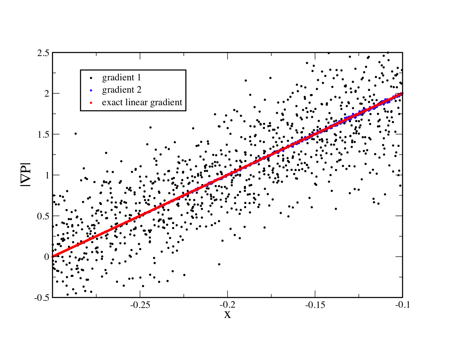
To illustrate the accuracy of different gradient estimates, we perform a simple experiment.
We distribute SPH particles, once on a hexagonal lattice and once via the regularization sweeps
described in Sec. 3.2.1, see Figs. 13 (right)
and 14 (middle), and assign them the same density and baryon number
and a pressure according to their positions with and .
Subsequently we calculate pressure gradients according to (”gradient 1”)
| (43) |
or (”gradient 2”)
| (44) |
or according to the exact linear gradient. The second estimate is just an SPH estimate of , see Eq. (6), which just subtracts the leading error term from Eq. (43). For the case where the particles are located on the hexagonal lattice all estimates yield accurate results and lie on the same straight line as they should. For the irregular particle distribution, the first gradient estimate produces a substantial scatter (black) around the exact result, see left panel Fig. 1. The second gradient estimate (blue) and the exact linear gradient result (red) are hard to distinguish by eye, but the latter produces errors that are approximately four orders of magnitude smaller (Fig. 1, right panel).

Noise trigger
Our aim is to find an additional trigger that indicates ”velocity noise” as it can appear behind
a shock. Such regions are characterized by some particles suffering expansion () while their
neighbors feel a compression (). Therefore, the ratio
| (45) |
can deviate from in a noisy region since contributions of different sign are added up in and therefore such deviations can be used as a noise indicator. To remain very local and to avoid an unnecessary smearing of the shock front, our summation in Eq. (45) only runs over neighbors within (our kernel extends to ). We use
| (46) |
where the quantity
| (47) |
should be zero without noise and our noise trigger becomes
| (48) |
For the noise reference value we use . The threshold for was introduced to
avoid triggering on acceptably tiny fluctuations around zero. Note that our choice of dissipation
parameters is on the “low-viscosity side” and sometimes can produce small, but in our opinion
acceptable, oscillations. This can be cured, of course, by applying more dissipation.
The quantities and are stored as an accurate indicators of whether
a particle is in a shock or a noisy region.
2.5 Smoothing kernel
Traditionally, most SPH formulations use the cubic spline (CS) kernel suggested by [31],
| (49) |
with , the number of spatial dimensions and the normalization (2/3 in 1D, in 2D and in 3D). It has been shown to yield good results over a large variety of test problems. This kernel, however, has the known shortcoming that its vanishing derivative at allows particles to ”pair” once they come close enough to each other, say in a shock. Often this has no dramatic effect, but it effectively reduces the resolution due to a poorer volume sampling by the SPH particles. Recent investigations [44, 54] find that kernels that are centrally peaked perform better in Kelvin-Helmholtz instabilities since they enforce a more regular particle distribution across the contact discontinuity. We find very good results in 1D with the CS kernel, but in 2D tests we also explore the performance of the centrally peaked ”Linear Quartic” (LIQ) kernel [54] in the form
| (50) |
with and and . The normalization constant is 2.962 in 2D and 3.947 in 3D. A comparison of both kernels and their derivatives is shown in Fig. 2. The results of our 2D shock test 8 favor the LIQ over the CS kernel.

2.6 Conversion between primitive and numerical variables
The new numerical variables, , and , obtained from the integration process, need to be converted into the physical quantities , , and . We follow the strategies of earlier special-relativistic approaches [29, 33]: all variables in the (polytropic) equation of state
| (51) |
are expressed as a function of the updated numerical variables and the pressure itself. The resulting equation is solved numerically for the new pressure which is subsequently used to recover the physical variables. From Eq. (18) and (23) one finds
| (52) |
and thus
| (53) |
Using Eq. (52) and Eq. (4) one can express the specific energy as
| (54) |
With aid of Eqs. (4) and (54) Eq. (51) can be solved for the new pressure that corresponds to the new values of the integrated numerical variables. Once is known, the Lorentz factor can be calculated from Eq. (53), the specific energy from Eq. (54) and the velocity from Eq. (52).
2.7 Time integration
We use the optimal third-order TVD algorithm to integrate the system of ordinary differential equations of the form . The solution is advanced by one time step to time according to
| (55) | |||||
| (56) | |||||
| (57) |
and we choose a simple error estimate to control the time step. Since the computing frame number density plays a central role in the discretization process we use it to measure the error growth rate:
| (58) |
where is the density estimate at obtained after a second-order Runge-Kutta step. The new time step is then chosen as . For the “safety factor” we use and for the tolerable error growth rate . We use this rather conservative time step choice in the tests presented below. We find, however, comparable results with a simpler time step choice similar to [8], where the time step, , is determined by the momentum change according to . In our experiments energy and momentum are conserved to about one part in .
2.8 Reference formulation
The performance of the new equation set is compared to the formulation of [8] which produces the best shock test results of all published SPH formulations that we are aware of333Note that [8] obtain their density estimate from integration rather than by summation.
| (59) | |||||
| (60) | |||||
| (61) |
where and
| (62) |
where they use a fixed value for their 1D tests. For the following comparisons we use their first suggestion for the signal velocity
| (63) |
their suggested alternative yields very similar results [8].
3 Numerical results
We use equal mass particles in our tests, so that the density information is encoded in the particle separation. Since SPH smoothes ”discontinuities” over a few resolution lengths, we consider it consistent with the spirit of the method to start a simulation from initial conditions that are smooth enough to be properly resolved by the method. Throughout the test bench, we approximate discontinuities in the initial conditions of a function via Fermi-functions
| (64) |
where and are the values to the left and right of the discontinuity
located at and is the characteristic transition length. We use half of
the average of the left and right interparticle separation for .
The issue of smoothed initial conditions is more a matter of taste than of technical
requirement. A comparison between simulations with as described and
shows only minor differences, see below.
Unless otherwise noted, about 3000 particles are shown and a polytropic equation of state
with an adiabatic exponent specific to each test is used.
3.1 Tests in 1D
3.1.1 Test 1: ”standard” relativistic shock tube


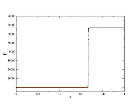
This mildly relativistic shock tube () has become a widespread benchmark
for relativistic hydrodynamics codes [29, 8, 50, 10, 30]. It uses a polytropic
exponent of , vanishing initial velocities everywhere, the left state has a pressure
and a density , while the right state is prepared with and .
The SPH result (circles, at t= 0.35) agrees excellently with the exact solution (solid line),
see Fig. 3. Only the contact discontinuity at is
somewhat smeared out. A striking difference to earlier SPH results [22, 51] is the absence
of any spike in and at the contact discontinuity. This is a result of the form of the dissipative terms,
Eqs. (27) and (28).
To explore the dependence of the results on the various new elements we perform the following low-resolution
(450 particles between -0.3 and 0.3) runs: i) use the new equation set, ii) the reference
equation set of Chow and Monaghan [8]
iii) the new equation set, but to explore the importance of the “grad-h”-terms
and iv) the new equation set, but (the value chosen in[8]) to explore the effect of the time-dependent viscosity parameters. With our parameters () the dissipation parameter reaches 0.57, so slightly larger than
the value chosen in [8] to ensure a fair comparison. The results are displayed in Fig. 4. All numerical parameters have exactly the same values in all cases.
Overall we find a good agreement between all the equation sets. For a
comparison we show the density since the shock-compressed shell is the most difficult structure
to capture and therefore shows the strongest deviations from the exact solution.

The ”grad-h” terms improve the left edge of the rarefaction fan (not shown in the figure) and
sharpen the left edge of the shock-compressed shell (black square vs. blue triangle). The time-dependent viscosity parameters are substantially reduced behind the shock which allows the density
peak level to reach closer to the correct value (black squares vs. green circles).
The main difference between the suggested and the reference equation set comes from the use of
the different signal velocity and the time-dependent dissipation parameters, the grad-h terms are
only a minor, though welcome, improvement.
We also briefly compare smoothed vs unsmoothed initial conditions, see beginning of Section 3.
To this end we use a low-resolution setup (about 700 particles) once smoothed using
in Eq. (64) and once without smoothing, .
Here / are the particle spacings on the left-/right-hand side. The result
for the quantity that showed in earlier approaches the largest deviations from the exact result, the specific energy ,
are displayed in Fig. 5. Overall, we find only minor differences.

3.1.2 Test 2: strong blast
The following test with initial conditions and is a more relativistic variant of a shock tube and was first considered by [40]. It poses a severe challenge since relativistic effects compress the post-shock state into a very thin and dense shell. The fluid in the shell moves at a velocity of which corresponds to a Lorentz factor of , the shock front moves with a velocity of 0.986, i.e. . This test has become a standard benchmark for relativistic schemes [40, 14, 28, 27, 29, 16, 55, 8, 13, 10, 3, 30].

Overall, the numerical solution (shown at t=0.16, 1800 particles) agrees well with the exact one, see Fig. 6. In particular, the intermediate states in velocity and pressure are well-captured. However, this difficult test is a severe challenge and the numerical solution
is not free of deficiencies. Somewhat large smearing in the internal energy occurs at , this is a result of using the maximum local eigenvalues rather than a proper spectral decomposition. Also, the numerical peak density value exceeds the exact one and the shock moves at a slightly too large velocity, effects that decrease with increasing numerical resolution. In comparison to [8] both these artifacts are substantially reduced, but nevertheless still present.
We again perform a set of test runs (400 particles
between -0.5 and 0.5): i) use the new suggested equation set, ii) the reference equation set of Chow and
Monaghan [8] iii) the new suggested equation set, but to explore the importance of
the “grad-h”-terms and iv) the new equation set, but (like in test ii) to explore
the effect of the time-dependent viscosity parameters. The results are displayed in
Fig. 7.

At the given resolution, the new formulation (black squares) clearly performs best. This is the only test where we see a clear improvement of the solution due to the grad-h terms (black squares vs. blue triangles). Again, controlling the amount of dissipation has a major effect, the schemes with constant dissipation (green circles and dashed line) show the least satisfactory performance.
3.1.3 Test 3: sinusoidally perturbed shock tube
Following [12], we explore a shock tube test whose initial right density state is sinusoidally perturbed:
| (65) |
The main goal of this experiment is to test the ability to transport smooth structures across
discontinuities. For this relatively mild shock only a moderate amount of dissipation is required,
we use . The numerical result at is displayed in Fig. 8 together
with the exact solutions of unperturbed shock tubes, once with a right hand side density value of
2.3 (dashed red line) and once with 1.7 (solid red line). Note the slightly larger shock speed in the latter case
( vs. ). The numerical solution
accurately reaches the correct levels of the limiting solutions in the shocked shell.

We perform again test runs to explore the influence of the equation sets and parameters (400 particles between 0 and 1): i) the new equation set, ii) the reference equation set of Chow and Monaghan [8] iii) the new equation set, but and iv) the new equation set, but , where for the constant--cases (ii and iv) we use the maximum value from run i) (=0.2).The conclusions from this test set are similar to the previous tests: the effects of the “grad-h-terms” are visible, but small and the effects from the time-dependent viscosity parameters are substantially more important. These tendencies are found in all of the subsequent numerical experiments.
3.1.4 Test 4: Ultra-relativistic wall shock
In this test cold gas moves relativistically towards
a wall. Upon hitting the wall, a shock front forms that travels upstream against the
inflowing gas leaving behind a hot and dense post-shock region with zero velocity.
In the ultra-relativistic limit () the shock travels at ,
i.e. for the polytropic exponent that we use in this test.
The post-shock values of density, pressure and specific energy are ,
, , where is the initial density.
We model the reflecting wall as “ghost” particles streaming with opposite velocity from the
right towards the wall located at . For this extremely strong shock we use . For the initial
gas velocity we use a value as high as corresponding to a Lorentz factor of
50 000! We further use and a specific energy of .
The results of the numerical calculation (1000 particles) at t=1 are shown together with the ultra-relativistic
limit values in Fig. 9.


The agreement between the numerical and the exact result is excellent, only the density and the specific energy show minor deviations from the exact solution (maximum error in density 1.2 %, in specific energy 1.1%) as a result of so-called “wall-heating” [40] near the boundary at x=1.
3.1.5 Test 5: Relativistic advection of a sine wave
In this test we explore the ability to accurately advect a smooth density pattern.
We choose a sine wave that propagates towards the right through a
periodic box. Since this test does not involve shocks, we switch off the artificial dissipation terms.
We use 500 equidistantly placed SPH particles in the interval [0,1], enforce periodic
boundary conditions and use a polytropic equation of state with . We
impose a computing frame number density , a
constant velocity corresponding to a Lorentz factor and we instantiate a constant pressure corresponding to
, where , and . The specific energies of the particles are chosen so that each particle has the same pressure .
The advection of this relativistic sine wave is essentially perfect, see Fig. 10:
the result after as many as 100 box crossings (circles) is indistinguishable from the initial setup
(red line), neither wave amplitude nor phase have been noticeably affected during the evolution.

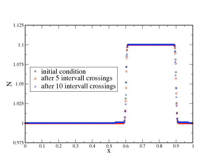
3.1.6 Test 6: Relativistic advection of a square wave
In this test we advect a square wave through the interval [0,1], again using periodic boundaries. Due to the involved steep flanks this problem is substantially more challenging than the previous one. We represent our box-shaped number density profile, , numerically as the sum of two Fermi-functions transiting from a lower state at to a higher state, , and back to the lower state at :
| (66) |
where sets the length scale on which the transitions occur. For the numerical experiments, we use , and is set to twice the particle spacing in the low density region. We use equal mass particles in this test, constant pressure throughout the
box is instantiated as in the sine wave problem above and we impose again a constant initial velocity of .
The results are displayed in Fig. 11: the black circles show the initial number
density profile, the results after 5 and 10 box crossings are shown as red circles and blue triangles, respectively. Overall the results of this challenging test agree very well with the initial state, but after 10 box crossings the flanks have slightly softened, and the low density state close to the flanks
has been slightly increased.
3.1.7 Test 7: Evolution of a relativistic simple wave
Here we present results of a challenging test that involves relativistic simple waves
and is rarely shown in the literature.
Relativistic simple waves [53, 15, 23, 2, 1] are characterized by
the spatial and temporal constancy of two of the three Riemann invariants for one dimensional
fluid flows. The three Riemann invariants are the specific entropy, , and the quantities
| (67) |
where is the sound speed and the x-component of the four velocity. Simple waves propagating to the right/left are characterized by the constancy of and . In this
test, a purely compressive initial sine pulse is set up that propagates into a static, uniform medium.
According to the results of [2], the initial velocity pulse will steepen while maintaining its
peak velocity until it evolves into a relativistic strong shock. From thereon,
the wave will dissipate and continuously decrease in velocity and in the contrasts of density and internal
energy (as measured with respect to the initial unperturbed state).
Our setup and parameter choice closely follows [2]. We use the equation of state of a
radiation-dominated fluid, . The initial
state consists of an unperturbed fluid state denoted by subscript with an overlaid ”velocity pulse”.
Like in [2], we choose the sound velocity in the unperturbed state as and display normalized, dimensionless quantities. For the initial (local rest frame) density we choose
and we use the length of our initial velocity pulse, , as characteristic length scale. The normalized quantities are denoted with a -symbol:
, where is the mass coordinate, , ,
, and .
We proceed in the following steps:
-
•
choose a sinusoidal velocity profile with a maximum as a function of . The width of the pulse in normalized mass coordinates is . To keep the pulse sufficiently far away from the (fixed) boundaries particles (at and 13), we choose as mass coordinate of the velocity maximum. For the ease of comparison, we plot the results with a constant -offset so that our initial setup (black curves in Fig. 12), coincides with the initial conditions of [2], see their Figure 5.
- •
-
•
and from this the specific energy and rest frame number density
(69) -
•
Finally, the computing frame baryon number density, , is calculated which, in turn, allows to assign positions and baryon numbers.
We display in Fig. 12 , , and , where the axis limits and output times are chosen as in Fig. 5 of [2]. The specific entropy is nowhere used in our SPH formulation, but can be post-processed for the chosen equation of state as .


Generally, we find very good agreement with the results of [2]. The initial sine-pulse continuously steepens while keeping its maximum velocity constant (to within about 2%) until
a relativistic shock forms (at ), see Fig. 12 upper left. Note in particular that the positions of the shock fronts agree excellently with those found in [2].
The wave subsequently dissipates, thereby producing a double peak structure in the density contrast
(at , upper right) with the dip coinciding with the peak in the entropy (lower right) and the
steep flank at in the specific energy (lower left). The entropy shows a small, spurious overshoot at the leading edge which is the result dividing and at the shock front, but apart from this, the agreement with [2] is very good.
We only find minor differences. Our simulations are less dissipative, the second density peak, for example, still exceeds the leading one at and is still visible at 7.40 while by the same time
it has vanished in [2]. Moreover, our specific energy at shows a clear plateau
behind the shock while theirs is a very smooth peak (which may just be the result of lower resolution),
and our entropy peak (at ) is slightly smaller than theirs ( vs. ).
3.2 Tests in 2D
Multi-dimensional calculations are complicated by the fact that the SPH particles have the
possibility to pass each other, which can cause imperfect particle distributions and numerical noise
(mainly in the velocity). And in fact, noise is a major concern for multi-dimensional SPH calculations.
Our strategy in this respect is threefold: a) since they can be a major reason for noise, we take particular
care to prepare accurate initial conditions, b) we have implemented an artificial dissipation
scheme that –in addition to shocks– also triggers on velocity noise, see Sect. 2.4.3, and iii)
we use relatively large values for the parameter in Eq. (11).
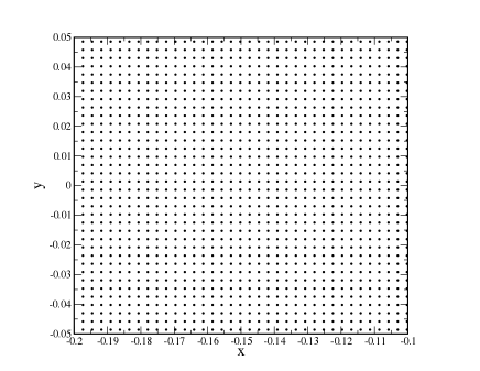
3.2.1 Initial particle distribution
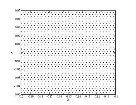
We have performed some experiments with the initial particle setup. We explored three types of initial particle distributions: i) a perfect equidistant grid, Fig. 13, left, ii) a hexagonal lattice, corresponding to the distribution of the centers of close-packed spheres, Fig. 13, right, and iii) a ”glass”-like particle distribution obtained in a relaxation process.
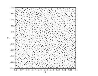
To produce the ”glass-like” distribution, we proceed in three steps: initially, the particles are distributed according to a Sobol quasi-random sequence [42], see Fig. 14, left panel. In a second step, we choose an ”adjustment time step”, , and perform several sweeps where we use the force law
| (70) |
which is a very simple discretization of the Euler equation. In each loop, the particle positions are updated according to
| (71) |
while the maximum value of the force is constantly monitored. This is done for as long as the
maximum force value is decreasing from one sweep to the next. Typically, the maximum force is reduced by
two orders of magnitude with respect to the initial Sobol sequence and provides a visually more regular
particle distribution, see middle panel in Fig. 14. Since the particles do
not move much during the optimization process, we store for each particle a (generous) candidate list
which is used for all the sweeps. Therefore, this procedure is a computationally inexpensive way to drive
the particles into a regular distribution. To further optimize the distribution, we ”relax” this particle
distribution to an optimal state by applying a large dissipation constant, , to the momentum, but not
the energy equation (we want to obtain a perfect particle distribution, but not artificially heat the
system). During this process, particles at the edges and, for shock tubes, near the transition between
the two states, are kept fix, so that each state relaxes separately.


In our tests we have found the best results with particles initially placed on the hexagonal lattice. The (somewhat artificial) particle distribution on a equidistant grid gave good shock tube results at low resolution, but at higher resolution produced a lot of velocity noise once the particles leave the grid. This effect was more pronounced for the peaked LIQ kernel, which we still prefer for the 2D tests since it performed slightly better in the below tests than the standard CS kernel.
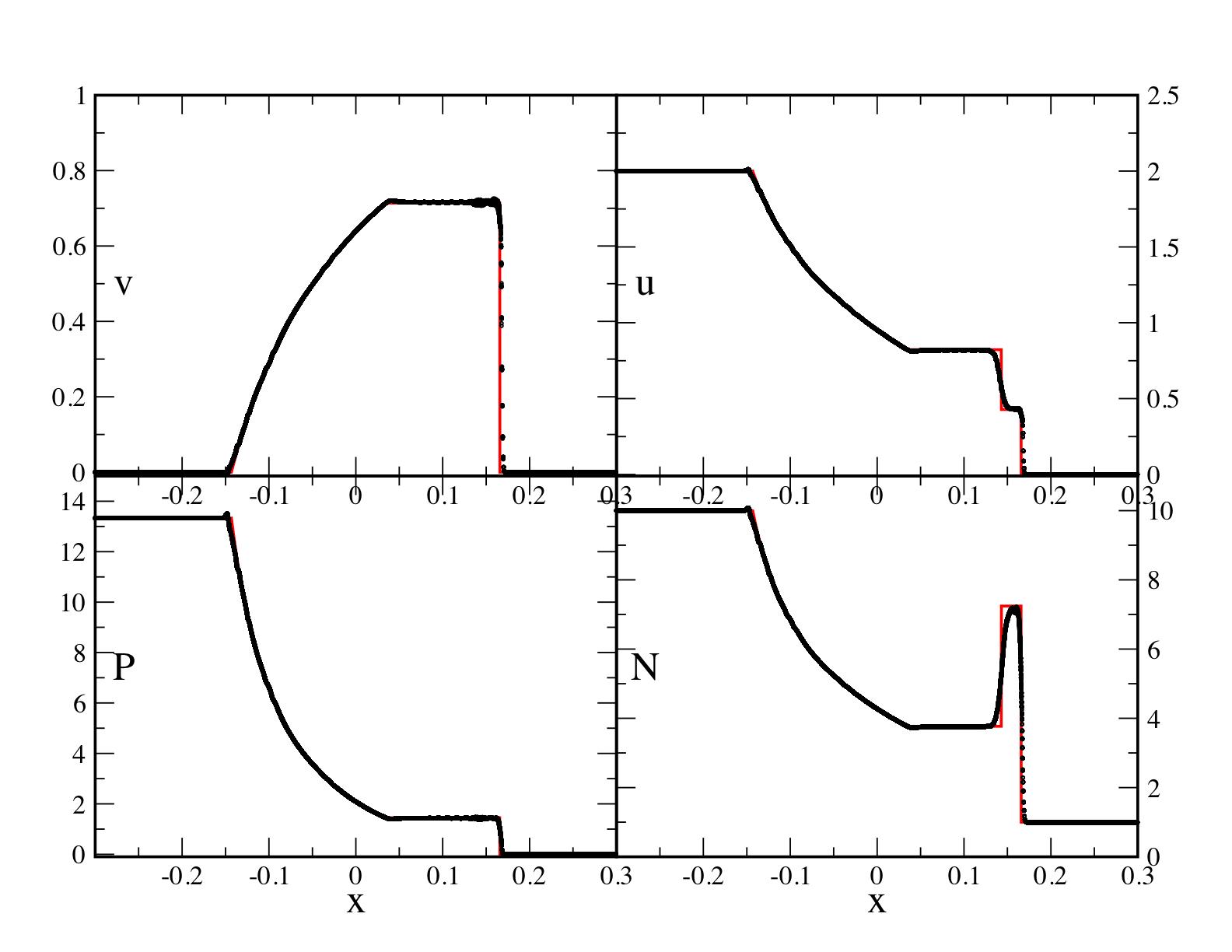
3.2.2 Test 8: 2D relativistic shock tube
This is the 2D version of test 1 shown above, i.e. the initial conditions are
and . For this test we place 140 000 particles on a hexagonal lattice
between [-0.4,0.4] [-0.02,0.02] and use our standard 2D parameter set:
together with the LIQ
kernel. The results are displayed in Fig. 15 with SPH particle properties as black circles
and the exact solution as red line. Generally, we find a
very good agreement with the exact solution, only the contact discontinuity is somewhat smeared out, similar
to the 1D case. Some small high-frequency oscillations in the velocity occur behind the shock front. They are
mainly caused by the particles that under the action of the peaked kernel have to change from the low density
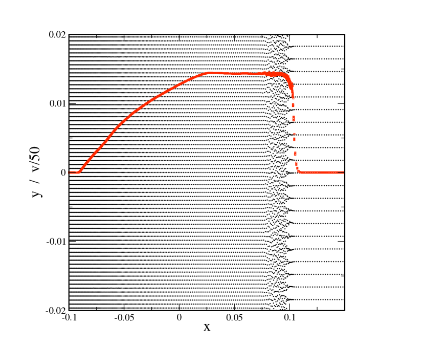
lattice into a higher density lattice. This is illustrated in Fig. 16 for a lower resolution
calculation (40 000 particles) where we have plotted the re-scaled velocities over the particle distribution.
The small post-shock irregularities in the velocity are clearly related to the transition region behind the
shock front at . They could be further reduced at the expense of applying more dissipation, but
we consider the current parameter set as a good compromise between low dissipation and absence of noticeable
post-shock oscillations.
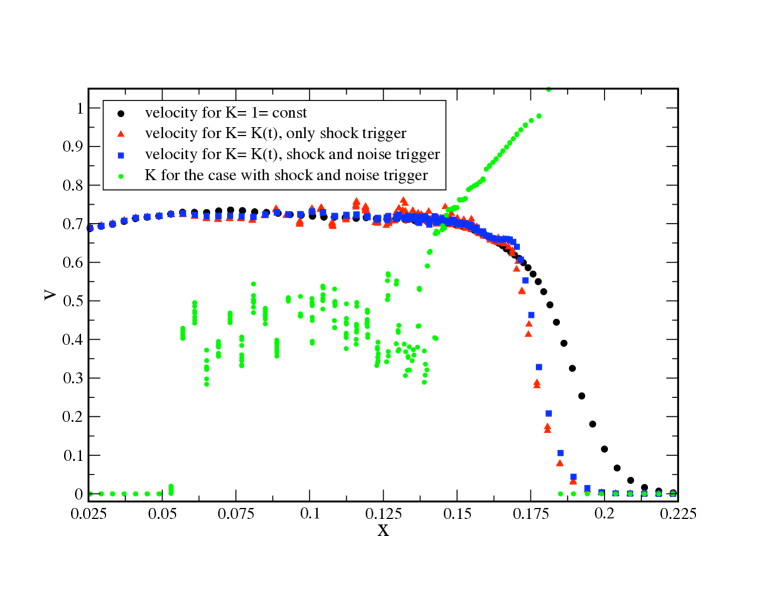
In the subsequent low-resolution tests (2000 particles), we illustrate the performance of the dissipation control scheme.
We perform all tests with and the
LIQ kernel. The results from the full scheme are shown in Fig. 17 as blue
squares. Note that the parameter (green circles) remains at zero up to the arrival of the shock front where it
jumps to values close to unity. In the post-shock region it remains around 0.5 (triggered by noise), and vanishes again in the expansion
fan. For comparison, we perform another test with identical parameters but with const everywhere (black circles),
and one more where we switch off the noise trigger (red triangles). Clearly, the new scheme substantially sharpens
shock fronts, essentially without compromising the post-shock region. With shock trigger only, the shock is sharp, but
substantial post-shock oscillations occur. The two independent triggers allow to apply a different amount of dissipation
to both phenomena.
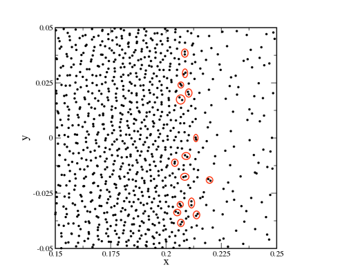
We also perform two tests to gauge the influence of the smoothing kernel, in the first one, we want to explore to
which extent ”pairing” of SPH particles occurs, in the second, we start from an imperfect initial particle
distribution and explore the influence of the kernel on the resulting velocity noise. The result of the
first experiment is shown in Fig. 18 where we zoom into the shock fronts of a low resolution
test, once with the CS and once with the LIQ kernel. In both cases the initial particle distribution is
obtained by the above described relaxation process. The CS kernel (left) produces many particle pairs
(some are highlighted by red ellipses) which deteriorates the volume sampling of the SPH particles. The
LIQ kernel (right), in contrast, produces only temporarily very few pairs directly at the shock front, but
the post-shock region is again sampled very regularly.

In the second test, we start from an imperfect initial particle distribution (10 000 SPH particles in 2D) as produced by the regularization sweeps, see above. The particles are subsequently assigned the properties that correspond to the left and right state and finally evolved, once with the CS and once with the LIQ kernel. The results at are shown in Fig. 19. The imperfect initial conditions introduce some scatter in the velocities (left), but the average values still agree very well with the exact solution. To assess the performance of the different kernels in this situation, we plot in Fig. 19, right panel, the deviation of the particle velocities, , from the exact solution, ,
| (72) |
The LIQ kernel (blue triangles) produces noticeably smaller errors than the ”standard” SPH kernel (red circles).

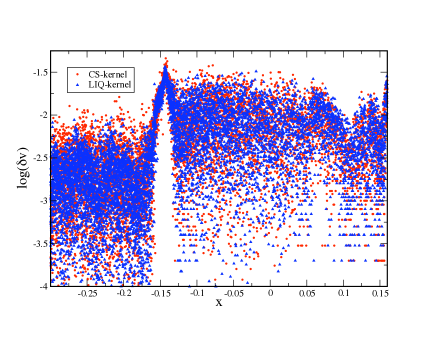
Summarizing our experiments with the two kernels, we find that the LIQ kernel performs slightly better, it produces a substantially more regular particle distribution and yields smaller errors for initially noisy particle configurations.
4 Summary
We have derived a new set of special-relativistic SPH equations from a variational principle. This
work differs from [36] in accounting also for the special-relativistic “grad-h” terms, corrections
for usually neglected derivatives of the smoothing kernels with respect to the resolution lengths.
We have used an artificial viscosity prescription that is inspired by Riemann solvers
[33]. We trigger independently on shocks and on velocity noise. Since the dissipation
applied in shocks is tuned according to the carefully measured density slope, shock fronts become
substantially sharper than for a constant dissipation parameter, see Fig. 17.
Contrary to earlier approaches [37, 48] we do not evolve
the dissipation parameter continously to the desired value, but instead increase it instantaneously, similar to the
approach of [9]. If not further triggered, the parameter subsequently decays to zero. None
of the triggers is specific to special relativity, both could be applied as well in Newtonian SPH.
We have carefully tested this new approach in a slew of numerical benchmark tests. We find that the
relativistic grad-h terms increase the accuracy of the method, but usually only have a moderate effect.
The improvements are generally dominated by the new signal velocity and the time-dependent
viscosity parameters. The new approach yields excellent results in the numerical experiments. As expected
for a purely Lagrangian scheme, it performs close to perfect in pure advection problems, even at large
Lorentz factors, see test problems 5 and 6. What is more, it also yields accurate results even in very strong
shock tests, which are usually considered a particular challenge for SPH. For example, the scheme is able to
accurately handle wall shock problems with a Lorentz factor as large as , see test 4. We
also perform a rarely shown, very challenging test in which a relativistic simple wave steepens into a strong
shock and subsequently dissipates (test 7). Our numerical results for this test are in close agreement
with those of the original paper [2].
In a last set of tests, we have explored the performance in 2D, relativistic shocks. Again we find very good
agreement with the exact solutions. In these multi-D tests we have also experimented with the peaked
linear quartic kernel [54] which yields slightly better test results than the most commonly
used cubic spline kernel. Numerical experiments [47] show that the scheme is
second-order accurate for smooth flows and first-order accurate if shocks are involved.
Acknowledgements
I want to thank SISSA (Trieste, Italy) and the Polytechnical University of Barcelona, UPC, for their
hospitality. It is a pleasure to acknowledge insightful discussions with Walter Dehnen, John Miller
and Justin Read.
This work has been supported by DFG under grant RO 3399/5-1.
References
- [1] A. M. Anile, Relativistic fluids and magneto-fluids, Cambridge Monographs on Mathematical Physics, Cambridge University Press, 1989.
- [2] A. M. Anile, J. C. Miller, S. Motta, Formation and damping of relativistic strong shocks, Physics of Fluids 26 (1983) 1450–1460.
- [3] P. Anninos, P. C. Fragile, Nonoscillatory Central Difference and Artificial Viscosity Schemes for Relativistic Hydrodynamics, ApJS 144 (2003) 243–257.
- [4] D. Balsara, von neumann stability analysis of smooth particle hydrodynamics–suggestions for optimal algorithms, J. Comput. Phys. 121 (1995) 357.
- [5] W. Benz, Smooth particle hydrodynamics: A review, in: J. Buchler (ed.), Numerical Modeling of Stellar Pulsations, Kluwer Academic Publishers, Dordrecht, 1990, p. 269.
- [6] A. Celotti, G. Ghisellini, M. Chiaberge, Large-scale jets in active galactic nuclei: multiwavelength mapping, MNRAS 321 (2001) L1–L5.
- [7] S.-H. Cha, A. P. Whitworth, Implementations and tests of Godunov-type particle hydrodynamics, MNRAS 340 (2003) 73–90.
- [8] J. E. Chow, J. Monaghan, Ultrarelativistic sph, J. Computat. Phys. 134 (1997) 296.
- [9] L. Cullen, W. Dehnen, Inviscid SPH, ArXiv e-prints.
- [10] L. Del Zanna, N. Bucciantini, An efficient shock-capturing central-type scheme for multidimensional relativistic flows. I. Hydrodynamics, A&A 390 (2002) 1177–1186.
- [11] K. Dolag, F. Vazza, G. Brunetti, G. Tormen, Turbulent gas motions in galaxy cluster simulations: the role of smoothed particle hydrodynamics viscosity, MNRAS 364 (2005) 753–772.
- [12] A. Dolezal, S. S. M. Wong, , J. Comp. Phys. 120 (1995) 266.
- [13] R. Donat, A Flux-Split Algorithm Applied to Relativistic Flows, Journal of Computational Physics 146 (1998) 58–81.
- [14] M. R. Dubal, Numerical simulations of special relativistic, magnetic gas flows, Computer Physics Communications 64 (1991) 221–234.
- [15] P. G. Eltgroth, Similarity Analysis for Relativistic Flow in One Dimension, Physics of Fluids 14 (1971) 2631–2635.
- [16] S. A. E. G. Falle, S. S. Komissarov, An upwind numerical scheme for relativistic hydrodynamics with a general equation of state, MNRAS 278 (1996) 586–602.
- [17] V. Fock, Theory of Space, Time and Gravitation, Pergamon, Oxford, 1964.
- [18] Y. A. Gallant, J. Arons, Structure of relativistic shocks in pulsar winds: A model of the wisps in the Crab Nebula, ApJ 435 (1994) 230–260.
- [19] R. A. Gingold, J. J. Monaghan, Smoothed particle hydrodynamics - Theory and application to non-spherical stars, MNRAS 181 (1977) 375–389.
- [20] S.-I. Inutsuka, Reformulation of Smoothed Particle Hydrodynamics with Riemann Solver, Journal of Computational Physics 179 (2002) 238–267.
- [21] A. Kheyfets, W. A. Miller, W. H. Zurek, Covariant smoothed particle hydrodynamics on a curved background, Physical Review D 41 (1990) 451–454.
- [22] P. Laguna, W. A. Miller, W. H. Zurek, Smoothed particle hydrodynamics near a black hole, ApJ 404 (1993) 678–685.
- [23] E. P. T. Liang, Relativistic simple waves - Shock damping and entropy production, ApJ 211 (1977) 361–376.
- [24] L. Lucy, A numerical approach to the testing of the fission hypothesis, The Astronomical Journal 82 (1977) 1013.
- [25] P. Mann, A relativistic smoothed particle hydrodynamics method tested with the shock tube, Computer Physics Communications.
- [26] P. Mann, Smoothed particle hydrodynamics applied to relativistic spherical collapse, Journal of Computational Physics 107 (1993) 188–198.
- [27] A. Marquina, J. M. Marti, J. M. Ibanez, J. A. Miralles, R. Donat, Ultrarelativistic hydrodynamics - High-resolution shock-capturing methods, A & A 258 (1992) 566–571.
- [28] J. Marti, J. Ibanez, J. Miralles, Phys. Rev. D 43 (1991) 3794.
- [29] J. Marti, E. Müller, J. Comp. Phys. 123 (1996) 1.
- [30] J. M. Marti, E. Müller, Numerical Hydrodynamics in Special Relativity, Living Reviews in Relativity 6 (2003) 7.
- [31] J. Monaghan, J. Lattanzio, A refined particle method for astrophysical problems, A&A 149 (1985) 135.
- [32] J. J. Monaghan, Smoothed particle hydrodynamics, Ann. Rev. Astron. Astrophys. 30 (1992) 543.
- [33] J. J. Monaghan, SPH and Riemann Solvers, Journal of Computational Physics 136 (1997) 298–307.
- [34] J. J. Monaghan, SPH compressible turbulence, MNRAS 335 (2002) 843–852.
- [35] J. J. Monaghan, Smoothed particle hydrodynamics, Reports on Progress in Physics 68 (2005) 1703–1759.
- [36] J. J. Monaghan, D. J. Price, Variational principles for relativistic smoothed particle hydrodynamics, MNRAS 328 (2001) 381–392.
- [37] J. Morris, J. Monaghan, A switch to reduce sph viscosity, J. Comp. Phys. 136 (1997) 41.
- [38] S. Muir, J. Monaghan, 3D Relativistic SPH, ArXiv Astrophysics e-prints.
- [39] R. Nelson, J. Papaloizou, Variable smoothing lengths and energy conservation in smooth particle hydrodynamics, MNRAS 270 (1994) 1.
- [40] M. L. Norman, K.-H. Winkler, Why ultrarelativistic numerical hydrodynamics is difficult, in: K.-H. Winkler, M. L. Norman (eds.), Astrophysical Radiation Hydrodynamics, Reidel, Berlin, 1986.
- [41] T. Piran, The physics of gamma-ray bursts, Reviews of Modern Physics 76 (2005) 1143.
- [42] W. H. Press, B. P. Flannery, S. A. Teukolsky, W. T. Vetterling, Numerical Recipes, Cambridge University Press, New York, 1992.
- [43] D. Price, Magnetic fields in astrophysics, Ph.D. thesis, University of Cambridge, arXiv:astro-ph/0507472 (2004).
- [44] J. I. Read, T. Hayfield, O. Agertz, Resolving mixing in smoothed particle hydrodynamics, MNRAS (2010) 767–+.
- [45] S. Rosswog, Astrophysical smooth particle hydrodynamics, New Astronomy Reviews 53 (2009) 78–104.
- [46] S. Rosswog, Relativistic smooth particle hydrodynamics on a given background spacetime, Classical and Quantum Gravity 27 (11) (2010) 114108–+.
- [47] S. Rosswog, Special-relativistic Smoothed Particle Hydrodynamics: a benchmark suite, eprint arXiv:1005.1679 (2010)
- [48] S. Rosswog, M. B. Davies, F.-K. Thielemann, T. Piran, Merging neutron stars: asymmetric systems, A&A 360 (2000) 171–184.
- [49] S. Rosswog, D. Price, Magma: a magnetohydrodynamics code for merger applications, MNRAS 379 (2007) 915 – 931.
- [50] S. Siegler, Entwicklung und untersuchung eines smoothed particle hydrodynamics verfahrens für relativistische strömungen, Ph.D. thesis, Eberhard-Karls-Universität Tübingen (2000).
- [51] S. Siegler, H. Riffert, Smoothed Particle Hydrodynamics Simulations of Ultrarelativistic Shocks with Artificial Viscosity, ApJ 531 (2000) 1053–1066.
- [52] V. Springel, L. Hernquist, Cosmological smoothed particle hydrodynamics simulations: the entropy equation, MNRAS 333 (2002) 649–664.
- [53] A. H. Taub, Relativistic Rankine-Hugoniot Equations, Physical Review 74 (1948) 328–334.
- [54] S. Valcke, S. De Rijcke, E. Roediger, H. Dejonghe, Kelvin-Helmholtz instabilities in Smoothed Particle Hydrodynamics, ArXiv e-prints.
- [55] L. Wen, A. Panaitescu, P. Laguna, A Shock-patching Code for Ultrarelativistic Fluid Flows, ApJ 486 (1997) 919–+.