Application of the MEGNO technique to the dynamics of Jovian irregular satellites

Abstract

We apply the MEGNO (Mean Exponential Growth of Nearby Orbits) technique to the dynamics of Jovian irregular satellites. The MEGNO indicator is an effective numerical tool to distinguish between quasi-periodic and chaotic orbital time evolution for a given dynamical system. We demonstrate the efficiency of applying the MEGNO indicator to generate a mapping of relevant phase-space regions occupied by observed jovian irregular satellites. The construction of MEGNO maps of the Jovian phase-space region within its Hill-sphere is addressed and the obtained results are compared with previous studies regarding the dynamical stability of irregular satellites. Since this is the first time the MEGNO technique is applied to study the dynamics of irregular satellites we provide a review of the MEGNO theory. We consider the elliptic restricted three-body problem in which Jupiter is orbited by a massless test satellite subject to solar gravitational perturbations. The equations of motion of the system are integrated numerically and the MEGNO indicator computed from the systems variational equations. An unprecedented large set of initial conditions are studied to generate the MEGNO maps. The chaotic nature of initial conditions are demonstrated by studying a quasi-periodic orbit and a chaotic orbit. As a result we establish the existence of several high-order mean-motion resonances detected for retrograde orbits along with other interesting dynamical features. The computed MEGNO maps allows to qualitatively differentiate between chaotic and quasi-periodic regions of the irregular satellite phase-space given only a relatively short integration time. By comparing with previous published results we can establish a correlation between chaotic regions and corresponding regions of orbital instability.

1 Introduction

The existence of natural satellites in orbit around Solar System giant planets has been known since Galileo discovered the four inner regular moons of Jupiter. Since then two classes of natural satellites have been identified to orbit the outer giant planets: regular and irregular satellites. The study of irregular satellites is interesting as they are located close to the Hill sphere boundary of the parent planet. Consequently Solar perturbations are present and chaotic behaviour is expected in the time evolution of their orbits. Recent reviews on the subject of irregular satellites are given in Peale (1999); Jewitt & Haghighipour (2007); Nicholson et al. (2008). Regular satellites are characterised by circular orbits located close to the equatorial plane of the planet. This is the case of the Galilean satellites of Jupiter. The class of irregular satellites differ in being on large eccentric and highly inclined orbits in either prograde (direct) or retrograde motion.

The majority of the current population of giant planet irregular satellites have been discovered by ground-based large aperture optical telescopes operating in dedicated survey programs over the past 10 years (Gladman et al., 1998, 2000, 2001; Sheppard & Jewitt, 2003; Holman et al., 2004; Sheppard et al., 2005, 2006). The most abundant irregular satellite population is observed to exist at Jupiter counting approximately 60 members at the current time. An interesting dynamical property of the phase space distribution of orbital elements is the clustering in distinct families for both prograde and retrograde irregular satellite members (Nesvorný et al., 2003, 2004).

The regular Galilean satellites are suggested to have formed by accretion processes within a circumjovian planetary disk (Canup & Ward, 2002; Mosqueira & Estrada, 2003; Estrada & Mosqueira, 2006). Observed kinematic differences between regular and irregular satellite orbits suggest a different formation mechanism of irregular satellites. The most favoured formation scenario is capture from an initial heliocentric orbit. The key element of permanent capture is the necessity of a frictional force (due to a gaseous environment) or energy transfer through close-encounter. Both processes are capable to dissipate orbital energy and provide a viable dynamical route to form a given population of irregular satellites. For a description of various capture scenarios we refer to Jewitt & Haghighipour (2007).

Several authors have studied general stability properties of irregular satellites. Haghighipour & Jewitt (2008) studied the region between Callisto and the innermost Jovian irregular satellite Themisto ($30~{}\,{\rm R}_{\rm Jup}<r<80~{}\,{\rm R}_{\rm Jup}$ where $\,{\rm R}_{\rm Jup}$ is Jupiters radius and $r$ is the distance of the satellite to Jupiter). Despite observational evidence indicating that this region is void of a satellite population they showed that a large fraction of this region renders possible satellite orbits stable for at least 10 Myrs. Extensive stability surveys of irregular satellites close to the Hill sphere of the giant planets have been carried out by Carruba et al. (2002); Nesvorný et al. (2003) by recording the lifetimes of irregular satellite test particles in various parameter surveys. Yokoyama et al. (2003) studied the region $250~{}\,{\rm R}_{\rm Jup}<r<370~{}\,{\rm R}_{\rm Jup}$ for prograde Jovian irregular orbits in the semi-major axis and inclination plane finding evidence of the presence of secular perturbations (Whipple & Shelus, 1993; Ćuk & Burns, 2004; Nesvorný & Beaugé, 2007). Stability properties of irregular orbits at the outer regions around the giant planet’s Hill sphere and beyond were studied by Shen & Tremaine (2008).

Motivated to study the phase space topology structure of irregular satellites in detail we applied the MEGNO chaos indicator (Cincotta & Simó, 2000; Goździewski, 2001; Goździewski et al., 2002) to qualitatively differentiate between quasi-periodic and chaotic phase space regions. Initial tests showed that MEGNO is efficient in showing chaotic regions using relative short integration times of the orbit. In this work we outline the basic principles of the MEGNO indicator as this is the first time this technique is applied to the dynamics of irregular satellites.

The structure of the paper is as follows. In section 2 we present the model and numerical methods used as well as initial conditions and definitions of angular variables. Section 3 presents a review of the MEGNO chaos indicator and an outline of its computation. Its relation to the Lyapunov exponent is reviewed and tests on numerical accuracy are presented. Section 4 describes the construction of dynamical maps of Jovian irregular satellites as studied in this work. Section 5 presents and outlines essential steps to obtain the secular system of the time variation of a satellite’s Keplerian elements using a time-averaged running window. Section 6 presents our results with comparison to previous work and section 7 concludes this work.

2 Model, numerical methods and initial conditions

The results obtained in this work are based on the elliptic restricted three-body problem. We integrate the equations of motion of the system (Morbidelli, 2002)

$$\frac{d^{2}\bm{r}_{i}}{dt^{2}}=-\frac{k^{2}m_{0}}{|\bm{r}_{i}|^{3}}~{}\bm{r}_{i}~{}+~{}\sum_{j=1,j\neq i}^{n}k^{2}m_{j}\Bigg{(}\frac{\bm{r}_{j}-\bm{r}_{i}}{|\bm{r}_{j}-\bm{r}_{i}|^{3}}-\frac{\bm{r}_{j}}{|\bm{r}_{j}|^{3}}\Bigg{)}.$$ (1)

Here $n=2$ in a jovian centric reference frame with $m_{0}$ denoting the mass of Jupiter and $k^{2}$ denotes the Gauss gravitational constant. The positions (relative to Jupiter) and masses of the satellite and the Sun are $(\bm{r}_{1},m_{1})$ and $(\bm{r}_{2},m_{2})$, respectively. In this model the satellite is orbiting Jupiter and its orbit is subject to Solar perturbations. In all integrations we regard the satellite as a test particle of zero mass. Oblateness effects from Jupiter are not considered in this model and perturbations from other planets are omitted as well. We consider this simplified model for two reasons. First the purpose of this paper is to demonstrate and apply the MEGNO chaos indicator to the dynamics of irregular satellites and secondly we aim to qualitatively identify chaotic regions originating from Solar perturbations only. If we were to include oblatenes and planetary perturbations cause and effect would be very difficult to isolate. The orbit of the satellite was obtained by the numerical integration of Eq. (1) using the 1) 15th-order Radau integration algorithm as implemented in the latest version of the MERCURY package (Chambers & Migliorini, 1997; Chambers, 1999) and 2) the Gragg-Bulirsch-Stoer (GBS) extrapolation algorithm (Hairer et al., 1993) as implemented in the CS-MEGNO code (Goździewski, 2001).

Figure 1: Graphical illustration of the relationship between angles in a heliocentric reference system and a planetocentric system. In both panels $\Upsilon$ denotes the reference direction from which inertial angles are measured and the orbital motion is counterclockwise. Panel A: Shows the orbit of (J)upiter with respect to the (S)un. Jupiters orbit is strongly exaggerated in its eccentricity for reasons of clarifications. In the current situation the longitude of pericenter of Jupiter is $\varpi_{J}^{hel}=135^{\circ}$. Panel B: The orbit of (S)un with respect to (J)upiter. Here the longitude of perijove $\varpi_{\odot}^{jov}=315^{\circ}$.

The Radau integrations were used to study individual satellite orbits on the long-time scales and the GBS integrator was used for the generation of MEGNO maps over the observed irregular satellite phase space region. Initial conditions (geometric cartesian elements relative to Jupiter’s centre of mass) for the Sun and observed irregular satellites have been obtained from the JPL Horizon Ephemeris generator (Giorgini et al., 1996) at the epoch 01-Jan-2005 (12:00 UT). It is worth to note that the Horizon Ephemeris generator cannot output osculating Keplerian elements of the Sun with respect to another object in the Solar System. Only cartesian vectors can be retrieved for the Sun relative to Jupiter. For the computations of the stability maps (see section 6.1) we have transformed the Sun’s cartesian elements to Keplerian elements using the mco_x2el.f subroutine as implemented in the latest version of MERCURY. The transformation introduces round-off errors not larger than $10^{-10}$ in the absolute errors which is much smaller than the error of observed elements of irregular satellites (e.g 15 meters in the semi-major axis). The retrieved initial conditions are referred to the ecliptic and mean equinox (xy-plane is the orbit of Earth) at reference frame ICRF/J2000.0. In this work we will present our results in a planetocentric reference system where Jupiter is at the centre and the ecliptic is the reference plane. Thus we denote the planetocentric elements of a satellite as $(a,e,I,\omega,\Omega,M)$ (where $M$ is the mean anomaly) and we use the subscript $\odot$ to indicate the Sun’s orbit relative to Jupiter and the subscript $J$ to denote the orbit of Jupiter in the heliocentric reference system. For the longitude of perijove of prograde irregular satellites we use the usual definition $\varpi=\Omega+\omega$. For retrograde satellites we use $\varpi=\Omega-\omega$. The mean longitude of an irregular satellite is then given by $\lambda=\varpi+M$.

In order to compare our data with previous published results in the literature using both planetocentric and heliocentric orbital elements we briefly point out the relationship of angles measured in the two reference frames. Changing the coordinate system from heliocentric to a jovicentric system leaves the semi-major axis and eccentricity unchanged as these quantities are invariable under a coordinate transformation. In Fig. 1 we demonstrate the relationship between the longitude of pericenter of the two bodies in the two reference system. If $\varpi_{J}^{hel}$ is the longitude of Jupiter in the heliocentric system and $\varpi_{\odot}^{jov}$ denotes the longitude of the Sun in the jovicentric system, then from geometric arguments we have $\varpi_{J}^{hel}=\varpi_{\odot}^{jov}+180^{\circ}$. A similar argument will lead to the relationship $\lambda_{J}^{hel}=\lambda_{\odot}^{jov}+180^{\circ}$ relating the mean longitudes of Jupiter and the Sun. The orbital inclination $(I_{\odot},I_{J})$ and the argument of node $(\Omega_{\odot},\Omega_{J})$ are unchanged under the transformation.

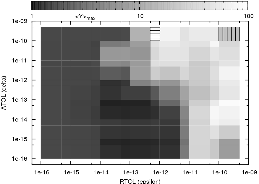
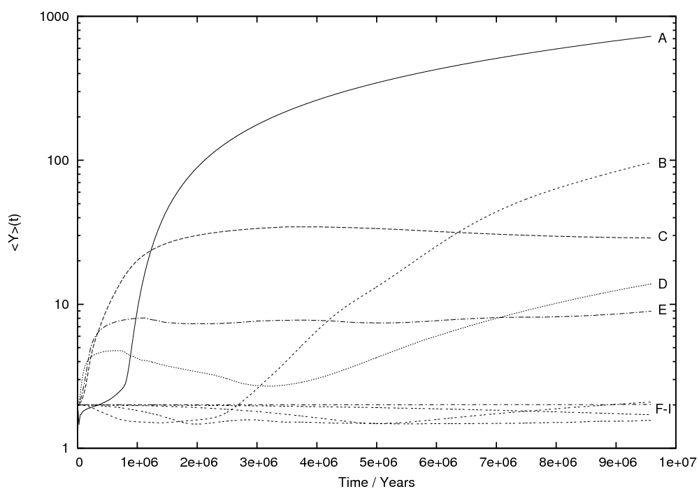
Figure 2: Results from 2-body Kepler integrations. Right panel: A) $\textnormal{(RTOL,ATOL)}=(5.0\cdot 10^{-11},\cdot 10^{-10})$, B) $\textnormal{(RTOL,ATOL)}=(5.0\cdot 10^{-13},\cdot 10^{-10})$, C) $\textnormal{(RTOL,ATOL)}=(1.0\cdot 10^{-11},\cdot 10^{-10})$, D) $\textnormal{(RTOL,ATOL)}=(1.0\cdot 10^{-10},\cdot 10^{-10})$, E) $\textnormal{(RTOL,ATOL)}=(5.0\cdot 10^{-11},\cdot 10^{-10})$, F) $\textnormal{(RTOL,ATOL)}=(1.0\cdot 10^{-16},1.0\cdot 10^{-16})$, G) $\textnormal{(RTOL,ATOL)}=(1.0\cdot 10^{-15},1.0\cdot 10^{-15})$, H) $\textnormal{(RTOL,ATOL)}=(1.0\cdot 10^{-14},1.0\cdot 10^{-10})$, I) $\textnormal{(RTOL,ATOL)}=(5.0\cdot 10^{-15},1.0\cdot 10^{-12})$. The area marked with vertical lines corresponds to case D and horizontal line corresponds to case B. The final value after 10 million years of $\langle Y\rangle$ for case F) was 1.999757, case G) 2.000367, case H) 1.636787 and case I) 1.798234.

3 The MEGNO chaos indicator

The time evolution of irregular satellite orbits exhibits both quasi-periodic and chaotic dynamics (Whipple & Shelus, 1993; Saha & Tremaine, 1993; Goldreich & Rappaport, 2003). An efficient numerical method to detect phase space regions resulting in chaotic or quasi-periodic initial conditions is provided by the MEGNO (Mean Exponential Growth of Nearby Orbits) factor (or indicator). The MEGNO technique was first introduced by (Cincotta & Simó, 2000; Cincotta et al., 2003) and were originally inspired from the concept of ‘conditional entropy of nearby orbits’ (CENO) (Cincotta & Simó, 1999; Gurzadyan, 2000). It can be applied to any dynamical system with more than two degrees of freedom and has found widespread applications in dynamical astronomy ranging from galactic dynamics to stability analysis of extrasolar planetary systems and Solar System small body dynamics (Cincotta et al., 2003; Goździewski, 2001, 2002, 2004; Breiter et al., 2005).

By numerically evaluating the MEGNO factor after a given integration time one obtains a quantitative measure of the degree of stochasticity of the system. One method (Morbidelli, 2002; Dvorak et al., 2005, and references therein) to discriminate between ordered (or regular) and chaotic (very often associated with orbital instabilities) satellite orbits, is the calculation of the system’s Lyapunov characteristic exponents (LCE) or Lyapunov characteristic numbers (LCN). From the theory of dynamical systems each system has a spectrum of Lyapunov exponents (possibly complex eigenvalues) each associated to a given eigenvector of the system. The Lyapunov exponents describe the rate of change of its corresponding eigenvector in time. The number of positive (or vanishing) Lyapunov exponents indicates the number of independent directions in phase space along which the satellite orbit exhibits chaotic (or quasi-periodic) behavior (Morbidelli, 2002). In particular, MEGNO is closely related to the maximum Lyapunov exponent (MLE or sometimes referred to maximum Lyapunov numbers, MLN) providing a quantitative measure of the exponential divergence of nearby orbits and belongs to the class of fast Lyapunov indicators (Morbidelli, 2002).

In this work, we apply the MEGNO criterion to the dynamics of Jovian irregular satellites. Details on the MEGNO concept and its numerical computation can be found in Cincotta et al. (2003) and Goździewski (2001). Since the MEGNO technique is applied for the first time to the dynamics of irregular satellites, we give a short review of the most important aspects of MEGNO and provide additional information on its numerical computation.

3.1 The Lyapunov Exponent

The maximum Lyapunov exponent $\gamma$, provides a useful quantitative measure to study the dynamical nature of the time evolution of a satellite orbit in phase space and is defined as

$$\gamma:=\lim_{t\rightarrow\infty}\frac{1}{t-t_{0}}\ln\Bigg{(}\frac{\delta(t)}{\delta(t_{0})}\Bigg{)}=\lim_{t\rightarrow\infty}\frac{1}{t-t_{0}}\int_{0}^{t}\frac{\dot{\delta}(s)}{\delta(s)}ds,$$ (2)

where $\delta(t)$ is the variational vector and measures the distance in phase space between two initially nearby orbits as a function of time. The second equality is easily realised by change of variables. For $\gamma>0$, an initial separation grows exponentially in time (definition of chaotic motion) at the rate $e^{\gamma t}$ or decays, if $\gamma<0$. In the case $\gamma=0$, the time rate of change of the variational vector $\dot{\delta}$ is 0. Since the (elliptic) restricted three-body problem is a conservative system the case $\gamma<0$ is never encountered and would indicate the presence of dissipative forces. In practical computations only a finite time estimate $\gamma(t)$ of $\gamma(s)$ is obtained after integration time $t$. In our computations, we will pay some attention on the proper choice of $t$. Usually the convergence of $\gamma$(t) is slow and a reliable numerical estimate of $\gamma$ requires a long integration time of the dynamical system. When exploring the dynamics of a large portion of phase space, short integration times are preferred when exploring the phase-space structure. For classic computations of the Lyapunov exponents from the variational equations we refer to (Benettin et al., 1980; Wolf et al., 1985).

3.2 Mathematical properties of MEGNO

A faster convergence property is obtained from the mean exponential growth factor of nearby orbits. The MEGNO indicator is closely related to the definition of $\gamma$ and is defined as

$$Y(t)=\frac{2}{t}\int_{0}^{t}\frac{\dot{\delta}(s)}{\delta(s)}~{}s~{}ds,$$ (3)

along with its time-averaged mean value

$$\langle Y\rangle(t)=\frac{1}{t}\int_{0}^{t}Y(s)~{}ds.$$ (4)

Cincotta & Simó (2000) showed that $\langle Y\rangle(t)$ converges faster to its limit value than the Lyapunov characteristic number. In the former definition the relative rate of change of the separation vector $\dot{\delta}/\delta$, is weighted with time during the integration giving preference to the memory of late evolutionary behavior of the separation vector (Morbidelli, 2002). The time-weighting factor introduces an amplification of any stochastic behavior, allowing an early detection of chaotic motion (Goździewski, 2001).

Computing the time evolution of Eq. (4) for a set of initial conditions allows the study of the dynamical properties in a given phase space region. Following Cincotta & Simó (2000); Cincotta et al. (2003), if the motion is of quasi-periodic nature, then $\delta$ grows linearly in time and $\langle Y\rangle$ will exhibit asymptotic oscillations about 2 for $t\rightarrow\infty$. In the case of chaotic initial conditions, $\langle Y\rangle(t)=\gamma t/2$ for $t\rightarrow\infty$. The latter equation relates the Lyapunov characteristic number to the limiting value of $\langle Y\rangle(t)$ at integration time $t$. A linear best fit to $\langle Y\rangle(t)$ would recover the Lyapunov characteristic number (Goździewski, 2001) . In summary, the time-averaged MEGNO ($\langle Y\rangle(t)$) converges faster to its limit value compared to the standard calculation of the Lyapunov characteristic number. This property allows a more rapid exploration of the dynamical phase space structure.

3.3 Numerical calculation of $Y(t)$ and $\langle Y\rangle(t)$

In practice, $Y(t)$ and $\langle Y\rangle(t)$ are calculated by rewriting Eqs. (3) and (4) into two differential equations (Goździewski, 2001)

$$\frac{dx}{dt}=\frac{\dot{\bm{\delta}}}{\bm{\delta}}~{}t~{}~{}~{}~{}~{}\textnormal{and}~{}~{}~{}~{}~{}\frac{dw}{dt}=2~{}\frac{x}{t},$$ (5)

where $Y(t)=2x(t)/t$ and $\langle Y\rangle(t)=w(t)/t$. To obtain $x(t),w(t)$ the two first-order coupled differential equations are solved along with the equations of motion. Initial condition for the variationals are chosen using a random generator. The quantities $\delta=\int\delta\dot{r}$ and $\dot{\delta}=\int\delta\dot{v}$ of the $i$’th body are obtained by solving the variational equations $\bm{\delta}=\delta\bm{v}$ and $\dot{\bm{\delta}}=\delta{\bm{\dot{v}}}$ (Mikkola & Innanen, 1999). At each time step we have for the $i-$th body the variationals

$$\delta\dot{r}_{i} = \delta v_{i}$$ (6)

$$\delta\dot{v}_{i} = -k^{2}(m_{0}+m_{i})\Bigg{(}\frac{\delta\bm{r}_{i}}{|\bm{r}_{i}|^{3}}-\frac{3\delta\bm{r}_{i}(\bm{r}_{i}\cdot\delta\bm{r}_{i})}{|\bm{r}_{i}|^{5}}\Bigg{)}-\delta\bm{A}_{i},$$ (7)

the first term describes the variation in the 2-body Kepler orbit and the variation in perturbations (or interactions) is

$$\delta\bm{A}_{i} = -\sum_{j\neq 0}^{i}m_{j}\Bigg{\{}\Bigg{[}\frac{\delta\bm{r}_{ij}}{|\bm{r}_{ij}|^{3}}-\frac{3\bm{r}_{ij}(\bm{r}_{ij}\cdot\delta\bm{r}_{ij})}{|\bm{r}_{ij}|^{5}}\Bigg{]}$$ (9)

$$-\Bigg{[}\frac{\delta\bm{r}_{0j}}{|\bm{r}_{0j}|^{3}}-\frac{3\bm{r}_{0j}(\bm{r}_{0j}\cdot\delta\bm{r}_{0j})}{|\bm{r}_{0j}|^{5}}\Bigg{]}\Bigg{\}}.$$

Here, $\bm{r}_{ij}=\bm{r}_{j}-\bm{r}_{i}$, $\delta\bm{r}_{ij}=\delta\bm{r}_{j}-\delta\bm{r}_{i}$ and $\delta\bm{r}_{0j}=\delta\bm{r}_{j}-\delta\bm{r}_{0}$, where the zero superscript denotes the central body. Eqs. (6)-(7) are computed in a straightforward way once the initial conditions have been defined for the variationals and the initial osculating orbits.

3.4 Numerical accuracy tests

The MEGNO indicator is numerically computed as outlined in the previous section using the Gragg-Bulirsch-Stoer integration algorithm (Hairer et al., 1993). All computations are carried out using double precision arithmetic. To control the numerical errors during computations two accuracy parameters are necessary for a GBS integration. The two parameters control the absolute $(\delta)$ and relative $(\epsilon)$ error tolerances for any given integration and both needs to be specified for a given accuracy requirement. In practical computations the usual choice of $(\delta,\epsilon)$ falls into the range from one part in $10^{9}$ down to the limit of the machine precision $(10^{-16})$ (depending on architecture). To find a suitable $(\delta,\epsilon)$ set, we integrated several 2-body Kepler problems for 10 million years by following the orbit of Himalia. In that case the motion is expected to be quasi-periodic, and we use it as a test case to determine confidence of the computed MEGNO indicator which should converge to $\langle Y\rangle(t)=2.0$. Initial numerical tests showed that the convergence of $\langle Y\rangle$ depends on the accuracy of the numerical integration. This property was already outlined in Goździewski (2001). We integrated Himalia’s orbit (without Solar perturbations) for different combinations of the tolerance parameters. In total we considered $(14\times 14)$ combinations with $(\delta,\epsilon)$ ranging from $10^{-10}$ to $10^{-16}$. The result of the integrations is shown in Fig. 2. The left figure panel shows the numerical value of $\langle Y\rangle$ (gray-scale color coded) at the end of the integration for a given combination of $(\delta,\epsilon)$. The right panel in Fig. 2 shows the time evolution of $\langle Y\rangle(t)$ of a few selected combinations of the tolerance parameters. The $(\delta,\epsilon)$ combinations resulting in the cases denoted by (A-E) are evidently of poor numerical accuracy showing $\langle Y\rangle\gg 2.0$ after 10 million years. We interpret this result as artificial numerical chaos, the result of the poor resolution of time descretisation in the integration algorithm. The cases (F,G,H,I) show a significant better agreement with the expected value of $\langle Y\rangle=2.0$ with some numerical fluctuation of $\langle Y\rangle$ observed during the integration. From the numerical experiments we fix $(\delta,\epsilon)=(10^{-16},10^{-15})$ for all MEGNO computations in the present work. In addition, we monitor the relative energy error $dE/E$ and note the maximum value reached during a given integration. For our choice of the tolerance parameters the average maximum relative energy error is on the order of $dE/E\sim 10^{-11}$ over 1 million years. By examining several spot tests on the time evolution of the relative energy error no systematic trends were observed only exhibiting a random walk over time. For all orbits the maximum relative energy error were smaller than $10^{-12}$ though in the restricted three-body problem this does not reflect the accuracy of the orbit of a massless test satellite. For that reason we follow the same approach as outlined in Nesvorný et al. (2003) and monitored the Jacobi constant during the numerical integration and found a maximum relative change of this quantity to be on the order of typically $10^{-6}$. We also computed the absolute error of the semi-major axis ($|a_{\odot}(t)-a_{\odot}|$) of the Sun and found it to be less than a few parts in $10^{-12}$. This means a preservation of 8 significant digits of the semi-major axis over 60000 years. Since we are not aiming at generating high-accuracy ephemerides of irregular satellite orbits we consider these tests as sufficiently reliable in order to establish confidence in our results presented in this work. In addition, uncertainties in observed orbital elements of irregular satellites are assumed to be much greater than rounding/truncation errors introduced by the numerical integration algorithm.

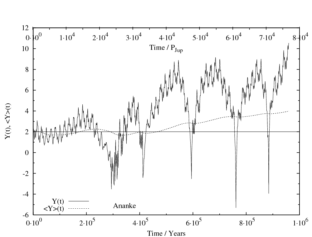
Figure 3: Time evolution of $Y(t)$ (solid curve) and $\langle Y\rangle(t)$ (dotted curve) from a numerical integration over 1 Myrs for the retrograde satellite Ananke including Solar perturbations. The solid horizontal line indicates $\langle Y\rangle=2.0$. The upper time line expresses integration time in units of Jupiters orbital period $\,{\rm P}_{\rm J}\approx 12.5$ yrs.

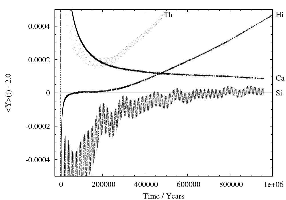
Figure 4: Time evolution of $\langle Y\rangle$ for different selected irregular satellites over a time scale of 1 million years. The shown satellites are Th(emisto), Hi(malia), Ca(rme) and Si(nope).

3.5 Numerical examples of test orbits and limitations

As an example Fig. 3 shows the time evolution of $Y(t),\langle Y\rangle(t)$ for the irregular satellite Ananke over a time span of 1 Myrs. In this integration, gravitational perturbations from the Sun were included and it is observed that Ananke’s orbit exhibits a weak sign of chaoticity. It is evident that no clear convergence of $\langle Y\rangle\rightarrow 2$ is observed. Also the time evolution of $Y(t),\langle Y\rangle(t)$ suggests that the time-averaged MEGNO $(\langle Y\rangle)$ is more reliable to indicate the presence of chaotic behavior as $Y(t)$ exhibits large variations about $Y(t)=2.0$ during the integration.

In Fig. 4 we show the results of calculating $\langle Y\rangle$ of four selected irregular satellites (Carme, Himalia, Sinope and Themisto) over 1 Myr. Our results suggest that both Themisto and Himalia (both on prograde orbits) shows chaotic behaviour as their calculated $\langle Y\rangle$ show clear sign of divergence from 2.0. The contrary is seen for the orbits of Carme and Sinope (both on retrograde orbits) indicating convergence (although slow for Carme) towards 2.0 indicating quasi-periodic time evolution. This result is in agreement with what is expected from numerical simulations. Prograde orbits tend to be less stable compared to retrograde orbits (Hamilton & Krivov, 1997; Nesvorný et al., 2003). It is noteworthy that although the calculation of $\langle Y\rangle$ is a powerful numerical tool for the detection of chaotic initial conditions it is necessary to be cautious when interpreting results. As mentioned previously two of the irregular satellites (Themisto and Himalia) show a weak sign of chaotic behaviour with $\langle Y\rangle$ diverging from 2.0 with $|\langle Y\rangle-2.0|<0.0003$ after 200000 years. In a MEGNO map such an initial condition would appear as quasi-periodic considered the large range in $\langle Y\rangle$ covering several orders of magnitude. Therefore it is imperative to point out that every numerical tool used to differentiate between quasi-periodic and chaotic behaviour is only capable of showing quasi-periodicity up to the integration time. On the contrary once chaotic behaviour (excluding numerical chaos) has been detected the orbit can be claimed chaotic for all times. If each initial condition in the MEGNO maps presented in this work were calculated on time scales similar to the age of the Solar System it is likely that no quasi-periodic orbits are detected. In our maps we can with high confidence associate chaotic regions with unstable orbits where the satellite either escapes or experience a collision with one of the inner moons or if the eccentricity grows high enough (due to the Kozai mechanism) the satellite may even collide with Jupiter itself.

4 Construction of MEGNO, ME, MS and MI maps

In this work we color code the MEGNO indicator on a 2-dimensional phase space section mapping out the dynamics of irregular satellites. In particular we show the dynamics in $(a,I)-$space, where $a$ is the semi-major axis and $I$ denotes the orbit inclination. We chose initial conditions in which orbit inclinations are relative to ecliptic (see IC section). For a given range in semi-major axis and inclination the grid of initial conditions in the maps are given by

Figure 5: Demonstrating the process of successive smoothing using a running window time average applied on the semi-major axis. See text for details.

$$a_{i}=a_{min}+\frac{\Delta a}{N_{x}}~{}i=a_{min}+\frac{a_{max}-a_{min}}{N_{x}}~{}i$$ (10)

and

$$I_{j}=I_{min}+\frac{\Delta I}{N_{y}}~{}j=I_{min}+\frac{I_{max}-I_{min}}{N_{y}}~{}j,$$ (11)

where $i=0,\ldots N_{x}$ and $j=0,\ldots N_{y}$ are integers defining the grid resolution. Chosing a large $(N_{x},N_{y})$ will result in a more detailed mapping of phase-space structures in $(a,I)$ space. The range in semi-major axis is chosen to span $a\in[0.04,0.20]$ AU ($[0.11,0.56]\,{\rm R}_{\rm H},[83,419]\,{\rm R}_{\rm Jup}$). Satellite inclinations cover the range $I\in[0,180]$ degrees considering both prograde and retrograde satellite orbits. In all MEGNO maps we chose to color code initial conditions resulting in quasi-periodic motion by blue (see the electronic version of this work). In the quasi-periodic case we have $|\langle Y\rangle-2.0|<0.01$ at the end of the numerical integration. In addition, we also provide maps showing the maximum eccentricity (ME) of an orbit at a given initial grid point. ME maps were constructed in parallel with the MEGNO calculations. The osculating elements were measured at each completed Jovian period and the maximum value is determined by comparing with a previous measurement of the eccentricity.

5 Smoothing orbital elements

To study the secular system of irregular satellites we have to filter out the fast frequencies. Saha & Tremaine (1993) already pointed out that the unfiltered variations in the action elements (semi-major axis, eccentricity and inclination) are larger than the filtered time series of a given element. This means that the fast variations (high-frequency terms) are much larger in amplitude than the slow variations (long-period terms). Hence the secular system is masked by the high frequencies. In this work an initial preliminary study of several test orbits confirmed this dynamical behaviour and we find that the most interesting dynamical features are to be found in the secular system. To obtain the secular system one can either average out the fast frequencies by applying a digital filter in either the time or frequency domain (Carpino et al. (1987); Quinn et al. (1991); Saha & Tremaine (1993); Michtchenko & Ferraz-Mello (1995)) or by simply averaging out all quasi-periodic oscillations with a running window average (Morbidelli, 1997; Morbidelli & Nesvorný, 1999).

In order to study the secular system we smooth the orbital elements of a given time sequence $A_{i}$ using the SMOOTH function as implemented in IDL. The smoothing procedure is a running window average applied on the full data set as obtained from a numerical integration. The output of a given numerical integration is given as a time sequence of orbital elements sampled at regular intervals of length $\Delta T$. For a given sequence of an orbital element

Figure 6: Time evolution of orbital elements for initial condition IC-I (left panel, chaotic) and initial condition IC-II (right panel, quasi-periodic). The full data set (panel a, c, e and g) and corresponding smoothed data set (panel b,d,f and h) are shown in each panel. From top to bottom panel: Semi-major axis (a+b). Eccentricity (c+d). Inclination (e+f) and the angle $\varpi-\varpi_{\odot}$ (g+h). The smoothing window applied to the data set in both panels are identical. Only the initial conditions has changed. Half of the window widths for a given element can be seen as a black bar at the beginning and end of the integration time. Each initial condition has been integrated for 60000 years corresponding to the integration length in the MEGNO maps. The window width are $w/2\times\Delta T=2500/2\times 40~{}\textnormal{days}=137$ years for panels b,d,g and $w/2\times\Delta T=20000/2\times\Delta T=1095$ years for panel f. Note that $\varpi_{\odot}=\varpi_{J}-180^{\circ}$.

$A_{i}=A(t_{i})$ with $t_{i}=t_{0}+i\Delta T$ (for $i=0,1,\ldots,N)$ the smoothed (secular) sequence ${R_{i}}$ is given by

$$R_{i}=\left\{\begin{array}[]{ll}\frac{1}{w}\sum_{j=0}^{w-1}A_{i+j-(\frac{w-1}{2})};&\textrm{ $i=\frac{w-1}{2},\ldots,N-\frac{w+1}{2}$.}\\ A_{i}&\textrm{otherwise.}\end{array}\right.$$

Here $N$ is the number of data points from the numerical integration and $w$ is the (running) window width over within which the original data set is averaged on. In units of time the window width is simply $w\Delta T$. The window width represents a free parameter and basically controls the supression of dynamical features seen in the data set: a too short window will have little smoothing effect and thus the fast frequencies are retained; a too large window width will suppress long-period features that appear on secular time scales. In practice some experimentation is needed in order to determine a satisfying window width. In this study we have performed an extensive survey of various window widths. In each plot showing smoothed orbital elements we have chosen the most appropriate window width in order to highlight the secular changes of a particular orbit.

Some care has to be taken when smoothing angular variables. As already mentioned by Saha & Tremaine (1993) filtering (or smoothing) an angular variable is problematic as angles may change discontinuously over the time sequence (i.e from $-\pi$ to $\pi$). Applying a running window smoothing procedure directly to an angular variable introduces spurious results around discontinuities. To circumvent this problem, we transform a given angular variable to a continuous signal. Let $\theta$ be an angular variable changing discontinuously at times during the numerical integration. Then we transform to the following continuous variables

$$p = A\cos(\theta)$$ (12)

$$q = -A\sin(\theta),$$ (13)

where $A$ is some suitable constant. Here we chose $A=1$. The IDL SMOOTH smoothing procedure is then applied to each of the quantities $p,q$ and we obtain $\bar{p},\bar{q}$ after which we obtain the smoothed angle $\bar{\theta}$ from $\bar{\theta}=\arctan(\bar{q}/\bar{p})$.

An important note about the SMOOTH routine is the following. The averaging behaviour at the beginning and end of the original time sequence depends on the optional edge_truncate keyword passed to the SMOOTH function. If this keyword is enabled the smoothing procedure might introduce false/misleading averages at the beginning and end of the smoothed signal. Details can be found in the IDL documentation. In addition if this keyword is disabled then it is important to note that $R_{i}=A_{i}$ for the first data points up to (but not including) $(w-1)/2$ and $R_{i}=A_{i}$ from $N-(w+1)/2$ (but not including) to $N$.

We demonstrate the effect of successively applying time-averaging smoothing windows to the time evolution of the semi-major axis in Fig. 5. Fig. 5a shows the whole signal over 60000 yrs with a sampling frequency of 40 days. At this stage a secular period of about 2400 years is clearly present in the frequency spectrum of the signal. Fig. 5b shows the first 200 years of the full data set (thin line) which is dominated by the orbital frequency of the satellite and an approximately 12 year period (Jupiter’s orbital period). When applying two successive smoothing windows to the raw data with window width 3 yrs and 12 yrs we obtain the average signal overplotted as a thick line in Fig. 5b. Fig. 5c shows a zoom of the smoothed signal over the whole integration time (note the difference in range of the semi-major axis). Fig. 5d (thin line) shows the first 3500 yrs of the previous signal. This time we detect a 34 year periodicity in the semi-major axis. Applying a smoothing window removes the 34 yr period (thick line in Fig. 5d) and the smoothed signal over the 60000 yrs is shown in Fig. 5e. Furthermore a 140 yr period signal is present in the semi-major axis as shown in Fig. 5. Applying a fourth smoothing window to the

Figure 7: MEGNO maps in $(a,I)$-space of test satellites with $e_{0}=0.20,\omega_{0}=0^{\circ},\Omega_{0}=0^{\circ},M_{0}=90^{\circ}$. The MEGNO indicator $\langle Y\rangle$ is color coded on a linear scale from 1.5 to 4 with $\langle Y\rangle=2$ indicating quasi-periodicity and $\langle Y\rangle=4$ denoting chaotic initial conditions. See the electronic version for colors. In both panels the symbols denote locations of irregular satellites. Themisto is at 0.05 AU ($0.14~{}\,{\rm R}_{\rm H},105~{}\,{\rm R}_{\rm Jup}$ and indicated by a $\times$ symbol). Himalia family = (+)-symbols and Carpo = (triangle) at 0.112 AU $(0.32~{}\,{\rm R}_{\rm H},235~{}\,{\rm R}_{\rm Jup})$. We plot family members for which $|e(t)-0.20|<0.05$. Ananke (black $\bullet$ symbols), Carme (pink rhomb symbols) and Pasiphae family (magenta square symbols). Left panel a: Three regions showing interesting dynamical features are shown by rectangles. Right panel b: High resolution zoom of the upper right region shown in panel a. Arrows indicate the locations of retrograde mean-motion resonances. Nominal locations in are given in Table  1. Also shown are the locations (IC-I and IC-II) of two test orbits. As already detected by Yokoyama et al. (2003) note the small stable region at $(a_{0},I_{0})=(0.142~{}\textnormal{AU},10^{\circ})$.

original raw signal now also removes this period and we end up with the secular signal (2400 yr period) shown in Fig. 5f.

In Fig. 6 we show examples of the effect of the smoothing procedure when applied to the numerical solution of two different initial conditions located close to each other in $(a,I)$-space. In both panels we show the semi-major axis, eccentricity, inclination and the angle $\varpi-\varpi_{\odot}$ for each initial condition. The left (right) panel is the result of integrating initial condition IC-I (IC-II) as indicated in Fig. 7. Each orbit were integrated for 60000 years, the integration length of each grid point in the MEGNO maps. The black bars (or sometimes scattered data points) shows half the window width (see figure caption for more details) and has been experimentally determined based on qualitative judgment with the goal to enhance the underlying dynamical changes in a given osculating element. As already pointed out in Saha & Tremaine (1993) we again observe that most of the variation in the orbital elements are found in the fast frequencies. A visual inspection of the time evolution of initial condition IC-I confirms its chaotic nature as correctly identified by MEGNO. For comparison a time-running window with identical window width has been applied to initial condition IC-II. Its quasi-periodic nature is clearly visible over the considered time span. From experimentation with the window width we observed that increasing the width averages out more and more quasi-periodic oscillations. No chaotic behaviour has been observed when increasing the window width. Following (Morbidelli & Nesvorný, 1999, p.301) by applying a time-running window smoothing procedure to a given osculating element we obtain the corresponding proper element. If the orbit evolves quasi-periodically (regular motion with a limited number of frequencies) in time then the corresponding proper element is a constant of motion. On the other hand if the corresponding proper element is chaotic then it exhibits a random walk in time. The chaotic nature of integrating initial condition IC-I particularly manifests itself in the time evolution of $\varpi-\varpi_{\odot}$ as shown in Fig. 6h (left panel). This angle repeatedsly changes from libration to circulation; this is characteristic of chaotic behaviour (i.e perturbed pendulum model). For comparison this angle circulates for initial condition IC-II (quasi-periodic) over the entire integration time span without any change in oscillation mode.

6 Results and discussion

6.1 MEGNO, $a_{max}$ and $e_{max}$ maps

Our results on computing the MEGNO indicator over a large grid in $(a_{0},I_{0})$-space is shown in Fig. 7. The figure shows the grid $(a_{0},I_{0})\in([0.04,0.20]~{}\textnormal{AU},[0.0^{\circ},180^{\circ}]$ region. The observed population of prograde and retrograde satellites are shown by various symbols (see figure caption for details). We obtained the osculating elements of the irregular satellites from the JPL Horizon Ephemeris system (see earlier section on initial conditions). We chose to consider this part of phase-space in order to compare with previous results as published by Carruba et al. (2002) and Yokoyama et al. (2003). These authors explore similar phase space regions although they consider a much smaller grid of initial conditions. Reproducing previously published results motivated us to apply and compute the MEGNO indicator over a much larger region occupied by the outer irregular Jovian satellites. In our work at initial time the eccentricity was set to $e_{0}=0.20$ and the remaining Kepler elements $(\omega_{0},\Omega_{0})$ were set to zero with $M_{0}=90^{\circ}$. We calculated the MEGNO indicator for 35100 initial conditions $(N_{x},N_{y})=(195,180)$. The orbit of each initial condition were integrated for $5\times 10^{3}\,{\rm P}_{\rm J}$ years ($\,{\rm P}_{\rm J}$ is the orbital period of Jupiter).

Figure 8: Maximum semi-major axis ($a_{max}$) of a given initial condition in $(a,I)$-space for a irregular test satellite. Left panel a: Same range in semi-major axis and eccentricity as for the MEGNO map with the maximum semi-major axis color coded in the range $[0.04,0.20]$ AU $([0.11,0.56]~{}\,{\rm R}_{\rm H},[84,419]~{}\,{\rm R}_{\rm Jup})$. Right panel b: Zoom of the rectangular area as indicated in the left a-panel figure.

MMR ($n:n_{J}$)	Nominal location (AU)	Order
4:1	0.203250	3
30:7	0.194113	23
9:2	0.187901	7
14:3	0.183400	11
19:4	0.181249	15
5:1	0.175156	4
21:4	0.169550	17
16:3	0.167779	13
27:5	0.166396	22
11:2	0.164372	9
17:3	0.161133	14
23:4	0.159573	19
6:1	0.155109	5
19:3	0.149618	16
13:2	0.147049	11
7:1	0.139961	6

Table 1: Nominal locations of retrograde MMRs as computed from Eq. (14). The masses of Jupiter and the Sun and the semi-major axis of Jupiter are taken from Murray and Dermott (Table A.1 and A.2).

To save computing time we stopped a given integration as soon as $\langle Y\rangle\geq 10.0$. The MEGNO indicator is then color-coded with $\langle Y\rangle=2.0$ indicating quasi-periodic motion and we only plot $\langle Y\rangle\leq 4$ to enhance the contrast of dynamical features in the transition region were the dynamics change from quasi-periodic to chaotic. Figure  7a shows several interesting regions of chaotic and quasi-periodic nature with unprecedented detail. We decided to compute high resolution maps to study this interesting region. A zoom plot is shown in Fig. 7b and corresponds to the area within the box in the upper right corner of Fig. 7a. The labels IC-I and IC-II correspond to initial conditions for two hypothetical (retrograde) irregular satellites.

Figure 9: Same as Fig. 8 but using $e_{max}$ for the colorcoding. Note the horizontal feature of enhanced eccentricity for both pro- and retrograde satellites. This feature was also reported to exists from a 1 Myr integration (Yokoyama et al., 2003, fig.6).

In parallel with computing $\langle Y\rangle$ to detect chaos we also recorded the maximum values of the test satellites semi-major axis and eccentricity every orbital period of the Sun. Fig. 8 and 9 show the corresponding maps. It is now apparent that the global chaotic region results in either escape or collisions after only $5\times 10^{3}\,{\rm P}_{\rm J}$ years. From this result we can conclude that the large chaotic region detected in the MEGNO map is strongly correlated with either escape from the Jovian Hill sphere or collisions with Jupiter itself. It is also interesting to note that over a large range the orbit size (semi-major axis) remains close to its initial value. Furthermore we also note that the locations of mean motion resonances are not visible in the zoom plot (Fig. 8b) as otherwise indicated by MEGNO. This indicates that the semi-major axis is unaffected by the presence of mean motion resonances and MEGNO is efficient in detecting mean motion resonances. A different picture is obtained when studying the maximum eccentricity attained during a numerical integration of a test satellite. Fig. 9 shows a clear dependence of $e_{max}$ with inclination. In a later section we will study and discuss the time evolution of these initial conditions to unravel their chaotic and quasi-periodic nature in detail presenting a proof-of-concept of detecting chaotic initial conditions. In this work we will discuss the location of mean motion resonances and postpone the study and discussion of other features (boxes located at polar and prograde orbits) in a future work.

6.2 Fine structure of mean-motion resonances

Fig. 7b shows details of the retrograde region with $a\in[0.14;0.20]$ AU $([0.39,0.56]~{}\,{\rm R}_{\rm H},[293,419]~{}\,{\rm R}_{\rm Jup})$ and $I\in[130^{\circ};180^{\circ}]$. Several vertical structures are observed corresponding to the location of chaotic mean-motion resonances. If $n$ and $n_{J}$ denotes the mean-motion of the satellite and Jupiter respectively, then the semi-major axis of a satellite in a $n:n_{J}$ mean-motion resonance with Jupiter is given by

$$a_{s}=a_{J}\Bigg{(}\frac{n}{n_{J}}\Bigg{)}^{-2/3}\Bigg{(}\frac{m_{J}+\,{\rm M}_{\odot}}{m_{J}}\Bigg{)}^{-1/3},$$ (14)

where $a_{J},m_{J}$ denote Jupiter’s semi-major axis and mass, respectively. $\,{\rm M}_{\odot}$ is the mass of the Sun. In the figure we show the location of several mean-motion resonances by arrows. See Table 1 for their nominal locations. Several high-order mean-motion resonances are detected.

When compared to the current population of observed irregular satellites it is interesting to note the large scatter in $(a,I)$ elements of the Pasiphae group. Fig. 7b strongly implies that several members of this group are strongly affected by the dynamics within high-order mean-motion resonances. The dynamical consequences of mean-motion resonances on the orbits of irregular satellites were already reported by Saha & Tremaine (1993) discussing the $n-6n_{J}\sim 0$ resonance of Sinope and possibly S/2001 J11 (Nesvorný et al., 2003). Showing a more compact distribution of the osculating elements members of the Carme family are on less inclined orbits $I\approx 165^{\circ}$. It appears that the dynamical effects of the mean-motion resonances occurs at a smaller magnitude for this group possibly having the effect of a smaller dispersion in orbital elements. In addition the Ananke group shows also a small scatter in their orbital elements possibly due to the close proximity of the 7:1 mean-motion resonance. The coincidence between the scatter of orbital elements of retrograde satellites and the presence of mean-motion resonances is probably not by chance. We stress that this work does not address the dynamical significance and effects of mean-motion resonances. Our results raises the question of the dynamical effects of mean-motion resonances on the orbital elements on a compact group of satellites. We will address this question in a future work and study the distribution of orbital elements of an initial compact group by gravitational scattering in mean-motion resonances.

6.3 Chaotic regions and Kozai mechanism

Figure 10: Secular time evolution of osculating elements from integrating IC-I. Elements $a,e$ were smoothed using a window width of $w\times\Delta T=2500\times 40~{}\textnormal{days}=274$ years. For the inclination $I$ we used $w=5000$. The black vertical bars shows half the window width. The elements $\varpi,\lambda$ denotes the (retrograde) longitude of pericenter and mean logitude of the satellite, respectively. $\rm P$ measures the orbital period of the satellite and $\,{\rm P}_{\odot}$ is the orbital period of the Sun in the jovicentric system. $\phi_{1}=5\lambda_{\odot}-\lambda-4\varpi_{\odot}$. $\phi_{2}=5\lambda_{\odot}-\lambda-2\varpi_{\odot}-2\varpi$. $\phi_{3}=5\lambda_{\odot}-\lambda-\varpi_{\odot}-\varpi-2\Omega_{\odot}$. $\phi_{4}=5\lambda_{\odot}-\lambda+2\varpi-6\Omega_{\odot}$.

From the MEGNO map (Fig. 7a), we observe a clear distinction between quasi-periodic and chaotic phase space regions. The general chaotic region for prograde satellites starts from $a=0.14~{}\textnormal{AU}~{}(0.39~{}\,{\rm R}_{\rm H},293~{}\,{\rm R}_{\rm Jup})$ and outwards. Stable quasi-periodic orbits for the retrograde satellites are found for orbits with semi-major axis up to 0.195 AU $(0.55~{}\,{\rm R}_{\rm H},409~{}\,{\rm R}_{\rm Jup})$. It is interesting to note that the chaotic phase-space of prograde satellites is larger when compared to the retrograde satellites. This asymmetry in $(a,I)$ space was already discussed by Nesvorný et al. (2003) pointing out the difference between prograde and retrograde stability limits. At larger semi-major axis the retrograde satellites are on dynamically more stable orbits when compared to the prograde irregular satellites. In this work the calculated MEGNO map confirms this stability asymmetry which is mainly explained by the existence of the evection resonance for prograde satellites (Nesvorný et al., 2003; Yokoyama et al., 2008, and references therein). In geometrical terms this resonance locks the satellites apocenter towards the direction of the Sun and maintains this alignment for a period of time. In this orbital configuration solar perturbations accumulate and the satellite eventually escapes from Jupiter when $\varpi-\lambda_{\odot}\sim 0$. An interesting feature shown in the map is the chaotic ‘horizontal cone’ for polar orbits at around $I\sim 90^{\circ}$ extending from $a=0.04~{}\textnormal{AU}~{}(0.11~{}\,{\rm R}_{\rm H},84~{}\,{\rm R}_{\rm Jup})$ to $a=0.12~{}\textnormal{AU}~{}(0.34~{}\,{\rm R}_{\rm H},251~{}\,{\rm R}_{\rm Jup})$. This region was already studied intensively by Carruba et al. (2002); Nesvorný et al. (2003) showing that test satellites with inclinations in the range $70^{\circ}<I<110^{\circ}$ are short-lived orbits with survival times less than $10^{7}$ years. Analytical perturbation theory (Carruba et al., 2002) showed that the accumulation of secular solar perturbations is the driving force causing the excitation of

Figure 11: Polar representation of the temporary circulation and librations of $\varpi-\varpi_{\odot}$ about $0^{\circ}$ ($\varpi-\varpi_{J}=180^{\circ}$) in the 5:1 mean-motion resonance of IC-I. The outer radius corresponds to $e\approx 0.33$ and the inner radius corresponds to $e\approx 0.41$. The alternation between libration and circulation is a clear sign of chaotic dynamics.

orbit eccentricity to large values. This mechanism is known as the Kozai resonance. Depending on the initial value of $\varpi$ circular orbits can reach high eccentricities and collisions with the inner regular satellites (or with Jupiter itself) are expected to occur. Thus the Kozai resonance provides an efficient dynamical mechanism to remove an initial population of near-polar irregular satellites. In near-polar orbits when studying Fig. 9 we notice that the Kozai regime is well identified with large eccentricities attained in the range $40^{\circ}<I<140^{\circ}$. However, it needs to be mentioned that the eccentricity excitations might strongly depend on the initial $\varpi$ (Carruba et al., 2002).

6.4 Chaoticity versus quasi-periodicity

Previously we have reported on the presence of chaotic dynamics as detected from calculating $Y,\langle Y\rangle$ on a grid of initial conditions in $(a,I)$-space. In the following we will study in detail two initial conditions that were detected to be either quasi-periodic or chaotic. Fig. 7 marks the two initial conditions by dots (surrounded by circles) with IC-I and IC-II. Both initial conditions have the same orbit inclinations with different semi-major axis. We refer to Table 2 for details on numerical values in the initial conditions. We have then numerically integrated both orbits using the Radau integrator with initial step size of 0.01 days and tolerance parameter of $10^{-}13$. Calculations were done in double precision enabling the ‘high’ output precision in MERCURY. Initial conditions for the Sun were obtained from the JPL Horizon Ephemeris. We sampled osculating elements every 40 days. To maintain consistency we integrated the orbits over $5\times 10^{3}~{}\,{\rm P}_{\rm J}$ years. For both orbits the maximum relative energy error at the end of integration were smaller than $10^{-13}$.

Figure 12: Time evolution of a test satellite with initial condition IC-II. The same window width were used as in Fig. 10. Note: The range in semi-major axis, eccentricity and inclination is smaller than in Fig. 10. This time the angle $\varpi-\varpi_{\odot}$ is circulating as opposed to the chaotic case.

Initial conditions	$a_{0}~{}(\textnormal{AU})$	$e_{0}$	$I_{0}~{}(^{\circ})$	Region
IC-I	0.173915	0.20	153.968	CH
IC-II	0.176179	0.20	153.968	QP

Table 2: Initial conditions for the two test satellites IC-I and IC-II in and close to the 5:1 mean-motion resonance as shown in Fig. 7. The remaining Kepler elements were set to $\omega_{0}=0^{\circ}$, $\Omega_{0}=0^{\circ}$ and $M_{0}=90^{\circ}$. CH and QP denotes initial conditions in the chaotic region and quasi-periodic region, respectively.

As suggested from MEGNO initial condition IC-I exhibits chaotic behaviour. We present the results of our single orbit calculation in Fig. 10 and Fig. 11. We have obtained those figures by successively applying the running window time average smoothing technique as outlined previously. In addition to the orbital elements $(a,e,I)$ we also plot the time variation of $\varpi-\varpi_{\odot}$ along with four critical angles $\phi_{1},\phi_{2},\phi_{3},\phi_{4}$ (see details in the figure caption). In the bottom panel of Fig. 10 we also show the time evolution of $Y,\langle Y\rangle$ as a function of time. We obtained this plot from a GBS integration. Quantitatively at time 60000 yrs $\langle Y\rangle\approx 18$ and a visual inspection shows a clear trend of divergence of $\langle Y\rangle$ over time. The presence of chaos is qualitatively best seen in the time evolution of the angle $\varpi-\varpi_{\odot}$. In Fig.  11 we give a polar representation of this angle. A similar approach was also adopted by Saha & Tremaine (1993). In the beginning this angle librates around $\varpi-\varpi_{\odot}=0^{\circ}$. After approximately 30000 years this libration mode switches into circulation for a short time period and then returns to the libration mode. At the end the angle circulates. This qualitative change between different modes of motion is characteristic of motion near a separatrix and hence chaotic motion is concluded. In the polar representation times of temporary librations are shown as ‘banana’-shape curves and circulations are indicated by full circles.

A more elongated banana corresponds to a larger libration amplitude of $\varpi-\varpi_{\odot}$. From Fig. 10 it is apparent that the libration amplitude changes with time. The initial conditions are chosen with the orbital inclination to be initially outside the Kozai resonance for which $\omega$ of the satellite starts to librate around either $90^{\circ}$ or $270^{\circ}$ (Carruba et al., 2002; Nesvorný et al., 2003; Yokoyama et al., 2003). No large eccentricity variations are expected. It is important to note the difference of the location of the libration centre found for the test satellite started at IC-I when compared to the libration behaviour of this angle for several major satellites. Saha & Tremaine (1993); Whipple & Shelus (1993) report that for the retrograde satellites Pasiphae and Sinope the angle $\varpi-\varpi_{J}$ librates about $180^{\circ}$. The difference from this work is the choice in reference system. In a heliocentric system the angle $\varpi-\varpi_{\odot}$ for IC-I would librate about $-180^{\circ}$ which is consistent with the general trend as reported in Saha & Tremaine (1993).

Figure 13: Polar representation of the $(a,I)-$space of Jovian irregular satellites for two different initial orbit eccentricities. Left panel: $e_{0}=0.10$. Right panel: $e_{0}=0.20$. In both panels the MEGNO indicator $\langle Y\rangle$ is color coded from 1.5 to 4.0 (see the electronic version for colors). The initial semi-major axis $(a_{0})$ is given in units of Jupiters Hill radius $\,{\rm R}_{\rm H}$, and $I_{0}$ denotes the initial orbit inclination. The diagonal lines represents orbit inclinations at $45^{\circ}$ (prograde satellites) and $135^{\circ}$ (retrograde satellites). The central vertical line represents the polar orbit at $I_{0}=90^{\circ}$. For comparison black dots indicate the initial conditions studied in (Carruba et al., 2002).

Since IC-I is near the 5:1 mean-motion resonance (compare with Table 1) we have systematically explored and looked for the existence of critical angles of the form Murray & Dermott (2001); Morbidelli (2002); Yokoyama et al. (2003)

$$\phi=k_{1}\lambda_{\odot}+k_{2}\lambda+k_{3}\Omega_{\odot}+k_{4}\Omega+k_{5}\varpi_{\odot}+k_{6}\varpi,$$ (15)

with $\sum k_{i}=0$ and the sum of the coefficients of the nodes being even as is required by the d’Alembert’s rules. The strength of a given critical angle depends on the power in eccentricity. From Fig. 10 we have $a_{max}$ then $\phi_{1},\phi_{2},\phi_{3},\phi_{4}$ circulates prograde sense.

Also whenever $I$ is minimum (maximum) then $e$ is maximum (minimum). Also whenever $\phi_{3}$ librates around $\pi$ then $I$ is at a minimum and constant (at time 35000 years). We also see that at the end of the time evolution of the satellite the angles $\phi_{1},\phi_{2}$ and $\phi_{3}$ are switching between libration around $\pi$ and prograde circulation. At some times we see a temporary resonance lock in $\phi_{2}$ in the 5:1 mean-motion resonance.

Turning our attention to the time evolution of the quasi-periodic orbit started at IC-II we report on the following results. Fig. 12 shows the smoothed time evolution of the osculating elements $(a,e,I)$ along with $\varpi-\varpi_{\odot}$. In the bottom panel plot we again plot the time evolution of $Y,\langle Y\rangle$ over 60000 years. The smoothing follows the running window time average techniques as outlined previously. Contrary to the chaotic orbit the angle $\varpi-\varpi_{\odot}$ now cirulates only and the secular time variation of the semi-major axis, eccentricity and inclination are characterised by quasi-periodic oscillations.

Based on the preceeding comparative study we conclude that MEGNO is a reliable numerical tool for detecting chaotic dynamics on short time scales. We plan to use this tool in future work on the dynamics of irregular satellites for the major planets in the Solar System. A particular interesting subject of study would be the change of mass of Jupiter and the corresponding change in the topology structure of phase-space at a given time during the growth phase of Jupiter.

6.5 Comparing with previous work

In the following we compared our MEGNO maps with numerical studies published previously in the literature. Fig. 13 shows a polar representation of Fig. 7a for two different values of initial eccentricities $e_{0}=0.10$ and $e_{0}=0.20$. In Fig. 13a,b the final value of $\langle Y\rangle$ after 60000 yrs of integration time is color coded with yellow indicating chaotic dynamical time evolution and blue indicating initial conditions exhibiting quasi-periodic dynamics. The dynamical and collisional evolution of irregular satellites and their lifetimes has been studied by Carruba et al. (2002) and Nesvorný et al. (2003). We have compared Fig. 13 with the results of long-term integrations of hypothetical irregular satellites conducted by Carruba et al. (2002, fig. 8, fig. 9). Similar studies can be found in (Nesvorný et al., 2003, fig. 9). Initial conditions of test satellites studied in Carruba et al. (2002) have been superimposed by black dots in both maps following the exact array of initial conditions as presented in Carruba et al. (2002). The initial semi-major axis ranges from 0.08 AU to 0.20 AU with spacing $\Delta a=0.02~{}\textnormal{AU}$. The initial inclination is $35^{\circ}$ to $70^{\circ}$ for the prograde and $110^{\circ}$ to $145^{\circ}$ for retrograde satellites with spacing $\Delta i=5^{\circ}$. In the following discussion it is important to stress the difference in the dynamical models used. In this work we only consider the Sun-Jupiter-test particle system without considering collisions with other bodies or ejections. Carruba et al. (2002) includes the perturbative effects of the major planets and includes collision and ejection criteria within Jupiter’s Hill sphere.

When comparing our results for prograde test satellites ($e_{0}=0.10$) with (Carruba et al., 2002, fig. 8) all test particles with lifetimes less than 10 Myrs $(a_{0}\geq 0.14~{}\textnormal{AU})$ are located in (or close to the onset of) the chaotic region shown in Fig. 13a. Initial conditions started in the quasi-periodic region have stable orbits over 1 Gyrs for low-inclination $(I_{0}\leq 50^{\circ},~{}a_{0}\leq 0.12~{}\textnormal{AU})$ orbits to 10 Myrs for high-inclination orbits $(I_{0}\geq 65^{\circ},~{}a_{0}\geq 0.08~{}\textnormal{AU})$. It is important to note that although our MEGNO map shown in Fig. 13a indicates quasi-periodic dynamics for the high-inclination orbits (for $a_{0}=0.08~{}\textnormal{AU}~{}\textnormal{to}~{}0.12~{}\textnormal{AU}$) those initial conditions are short-lived due to the presence of the Kozai cycle which opens up a route for those satellites to reach into the region of the orbits of the Gallilean satellites. As demonstrated by Carruba et al. (2002) such high-inclination test satellites will experience close encounters or collisions with the massive regular satellites of Jupiter. For the retrograde orbits (with $e_{0}=0.10$) a comparison allows the conclusion that all test satellites started in (or close to) the chaotic region have lifetimes smaller than 1 Gyrs and all test satellites with initial conditions in the quasi-periodic region have lifetimes over 1 Gyr with the exception of high-inclination orbits exhibiting Kozai cycles in their orbital eccentricities and inclinations. Similar conclusion are obtained when comparing the results shown in Fig. 13b $(e_{0}=0.20)$ with (Carruba et al., 2002, fig. 8). A final interesting point to mention is the qualitative difference in $(a,I)$-phase space topology of irregular satellites when varying the initial eccentricity. The prograde quasi-periodic region seen in Fig. 13a at $I_{0}\leq 35^{\circ}$ with $a_{0}/\,{\rm R}_{\rm H}\times\cos(I_{0})\approx 0.4$ has significantly decreased in Fig. 13b when $e_{0}=0.20$. Furthermore the 5:1 MMR for retrograde orbits manifests itself more prominently in Fig. 13b when compared to Fig. 13a. This suggests that the structure of $(a,I)$-phase space topology is strongly dependent on initial eccentricity and a survey of this region of parameter space is currently ongoing.

7 Discussion and conclusions

We have introduced, described and applied the MEGNO chaos indicator to the dynamics of jovian irregular satellites. Our results are based on the elliptic restricted three-body problem considering a test particle (irregular satellite) in a jovian planetocentric reference system perturbed by the Sun on an elliptic orbit. Initial conditions for the numerical integrations of the orbits have been obtained from the JPL Horizon Ephemeris Generator. Basic concepts and properties of MEGNO are reviewed and described as well as details on the practical computation of $Y(t)$ and $\langle Y\rangle(t)$ based on the variational equations. Numerical tests (see Fig. 2) have been carried out to detect and avoid artificial numerical chaos arising from the natural time discretisation of the applied numerical integration algorithms. Our test determined an optimal choice in the absolute and relative error tolerances required in the Gragg-Bulirsh-Stoer algorithm to detect real chaotic dynamics. We have calculated the MEGNO factor for several known irregular satellites for the prograde and retrograde cases. Our calculation suggests that prograde satellites are more chaotic in contrast to retrograde orbits (see Fig. 4) though the detected chaos is very weak. To clarify this suggestion more detailed computations including also additional planetary perturbations along with Solar tides are necessary. Such calculations resulting in an estimate of the Lyapunov indicator are currently in progress for the major irregular satellites.

It is important to note that every numerical tool capable of distinguishing between quasi-periodic and chaotic dynamics has limitations with regards to claiming quasi-periodicity considering only a limited period of time. This certainly is also the case for the MEGNO technique. In Fig. 3 we computed $Y(t)$ and $\langle Y\rangle(t)$ for the retrograde irregular satellite Ananke. The plot shows that after 1 Myr the orbit of Ananke exhibits a chaotic orbit with $\langle Y\rangle(1~{}\textnormal{Myr})\approx 4.0$. In the 60 kyr integrations the orbit of Ananke would possibly be interpreted as quasi-periodic with $\langle Y\rangle(t)$ deviating only slightly from 2.0.

Considering 35100 orbits we calculated the MEGNO indicator on a large grid in $(a,I)$-space known to be occupied by observed irregular satellites (Fig. 7). The resulting map revealed several interesting dynamical structures and we compared our results with previous studies addressing the question of the orbital stability of jovian test satellites. We found good qualitative agreement between chaotic (quasi-periodic) and unstable (stable) regions as was found previously (Carruba et al., 2002; Nesvorný et al., 2003). In particular we confirm the asymmetry of the stable region when comparing prograde and retrograde satellite orbits Nesvorný et al. (2003). Retrograde satellite orbits have access to a larger volume of phase space characterised by orbit stability. This result is in contrast to the prograde satellites for which chaotic orbits and its associated instability occurs (for $e_{0}=0.20$) at $a\approx 0.13$ AU $(0.37~{}\,{\rm R}_{\rm H},272~{}\,{\rm R}_{\rm Jup})$ and onwards (cf. Fig. 7). A small region of $(a,I)$-space at $a\approx 0.14$ AU have been detected to indicate quasi-periodicity. In addition we detected the presence of mean motion resonances of retrograde satellites with the Sun. The location of several high order mean motion resonances were determined and compared with the present population of retrograde irregular satellite families. We find that the orbital elements of the members of the Pasiphae family are largely scattered as opposed to the Carme group exhibiting to occupy a more compact region in $(a,I)$-space. We preliminary explain this excess in scatter of the osculating elements due to the close proximity to mean-motion resonances. This postulate will be subject to a separate study currently ongoing addressing the question whether high-order (retrograde) mean motion resonances are capable of dispersing an initial compact group of satellite members.

To support our results obtained from MEGNO we also calculated and compared two initial conditions associated to two retrograde satellite orbits. The first were chosen to be close to the 5:1 mean-motion resonance and the second initial condition were chosen to be just outside the location of this resonance. We then searched for signs of chaoticity and quasi-periodicity to validate the results obtained from calculating MEGNO. Applying a time-running smoothing window on the osculating elements our analysis of the single orbit computations support the results obtained from MEGNO. Initial conditions started in chaotic regions are associated to libration/circulation of resonant angles. Quasi-periodic initial conditions show only circulating behaviour.

Motivated by the success of applying the MEGNO technique to the dynamics of irregular satellites we plan to conduct a large parameter survey to identify further chaotic regions within the Hill sphere of Jupiter. In addition we plan to include giant planet perturbations and generate similar MEGNO maps of observed populations of irregular satellites in orbit around the remaining giant planets in the Solar System.

References

- Benettin et al. (1980) Benettin G., Galgani L., Giorgilli A., Strelcyn J.-M., 1980, Meccanica, 15, 9
- Breiter et al. (2005) Breiter S., Melendo B., Bartczak P., Wytrzyszczak I., 2005, aap, 437, 753
- Canup & Ward (2002) Canup R. M., Ward W. R., 2002, AJ, 124, 3404
- Carpino et al. (1987) Carpino M., Milani A., Nobili A., 1987, AA, 181, 182
- Carruba et al. (2002) Carruba V., Burns J., Nicholson P., Gladman B., 2002, Icarus, 158, 434
- Chambers (1999) Chambers J., 1999, MNRAS, 304, 793
- Chambers & Migliorini (1997) Chambers J., Migliorini F., 1997, BAAS, 27-06-P
- Cincotta et al. (2003) Cincotta P., Giordano C., Simó C., 2003, Physica D, 182, 151
- Cincotta & Simó (1999) Cincotta P., Simó C., 1999, CMDA, 73, 195
- Cincotta & Simó (2000) Cincotta P., Simó C., 2000, ApJS, 147, 205
- Ćuk & Burns (2004) Ćuk M., Burns J., 2004, AJ, 128, 2518
- Dvorak et al. (2005) Dvorak R., Freistetter F., Kurths J., 2005, Chaos and Stability in Planetary Systems. Lect. Notes Phys. 683, Springer Verlag, Berlin
- Estrada & Mosqueira (2006) Estrada P. R., Mosqueira I., 2006, Icarus, 181, 486
- Giorgini et al. (1996) Giorgini J. D., Yeomans D., Chamberlin A. B., Chodas P., Jacobson R. A., Keesey M. S., Lieske J., Ostro S., Standish E., Wimberly R., 1996, BAAS, 28, 1158
- Gladman et al. (1998) Gladman B. J., et al., 1998, Nature, 392, 897
- Gladman et al. (2000) Gladman B. J., et al., 2000, Icarus, 147, 320
- Gladman et al. (2001) Gladman B. J., et al., 2001, Nature, 412, 163
- Goldreich & Rappaport (2003) Goldreich R., Rappaport N., 2003, Icarus, 166, 320
- Goździewski (2001) Goździewski K., 2001, A&A, 378, 569
- Goździewski (2002) Goździewski K., 2002, A&A, 393, 997
- Goździewski (2004) Goździewski K., 2004, ApJ, 610, 1093
- Goździewski et al. (2002) Goździewski K., Bois E., Maciejewski A. J., 2002, MNRAS, 332, 839
- Gurzadyan (2000) Gurzadyan V.G.and Ruffini R., 2000, The Chaotic Universe: roceedings of the Second ICRA Network Workshop. World Scientific Publishing, ISBN-13: 978-9810242558
- Haghighipour & Jewitt (2008) Haghighipour N., Jewitt D., 2008, AJ, 136, 909
- Hairer et al. (1993) Hairer E., Norsett S., Wanner G., 1993, Solving ordinary differential equations I. nonstiff problems, 2nd edition.. Springer Series in Computational Mathematics, Springer-Verlag, see also http://www.unige.ch/math/folks/hairer/
- Hamilton & Krivov (1997) Hamilton D. P., Krivov A. V., 1997, Icarus, 128, 241
- Holman et al. (2004) Holman M. J., et al., 2004, Nature, 430, 865
- Jewitt & Haghighipour (2007) Jewitt D., Haghighipour N., 2007, ARA&A, 45, 261
- Michtchenko & Ferraz-Mello (1995) Michtchenko T., Ferraz-Mello S., 1995, AA, 303, 945
- Mikkola & Innanen (1999) Mikkola S., Innanen K., 1999, CMDA, 74, 59
- Morbidelli (1997) Morbidelli A., 1997, Icarus, 127, 1
- Morbidelli (2002) Morbidelli A., 2002, ”Modern Celestial Mechanics - Aspects of Solar System Dynamics”. Taylor & Francis
- Morbidelli & Nesvorný (1999) Morbidelli A., Nesvorný D., 1999, Icarus, 139, 295
- Mosqueira & Estrada (2003) Mosqueira I., Estrada P. R., 2003, Icarus, 163, 198
- Murray & Dermott (2001) Murray C., Dermott S., 2001, Cambridge Univserity Press
- Nesvorný et al. (2003) Nesvorný D., Alvarellos J. L. A., Dones L., Levison H. F., 2003, AJ, 126, 398
- Nesvorný & Beaugé (2007) Nesvorný D., Beaugé 2007, AJ, 133, 2537
- Nesvorný et al. (2004) Nesvorný D., Beaugé C., Dones L., 2004, AJ, 127, 1768
- Nicholson et al. (2008) Nicholson P. D., Cuk M., Sheppard S. S., Nesvorny D., Johnson T. V., 2008, The Solar System Beyond Neptune. University of Arizona Press
- Peale (1999) Peale S., 1999, ARA&A, 37, 533
- Quinn et al. (1991) Quinn T., Tremaine S., Duncan M., 1991, AJ, 101, 2287
- Saha & Tremaine (1993) Saha P., Tremaine S., 1993, Icarus, 106, 549
- Shen & Tremaine (2008) Shen Y., Tremaine S., 2008, AJ, 136, 2453
- Sheppard et al. (2005) Sheppard S. S., et al., 2005, MPEC 2005-J13
- Sheppard & Jewitt (2003) Sheppard S. S., Jewitt D. C., 2003, Nature, 423, 261
- Sheppard et al. (2006) Sheppard S. S., Jewitt D. C., Kleyna J., 2006, MPEC 2006-M44, 2006-45, 2006-M48
- Whipple & Shelus (1993) Whipple A. L., Shelus P. J., 1993, Icarus, 101, 265
- Wolf et al. (1985) Wolf A., Swift J. B., Swinney H. L., Vastano J. A., 1985, Physica D, 16, 285
- Yokoyama et al. (2003) Yokoyama T., Santos M., Cardin G., Winter O., 2003, A&A, 401, 763
- Yokoyama et al. (2008) Yokoyama T., Viera Neto E., Winter O.C Sanchez D. M., de Oliveira Brasil P., 2008, Mathematical Problems in Engineering, 2008, 16