Onsager coefficients of a finite-time Carnot cycle

Abstract

We study a finite-time Carnot cycle of a weakly interacting gas which we can regard as a nearly ideal gas in the limit of $T_{\mathrm{h}}-T_{\mathrm{c}}\to 0$ where $T_{\mathrm{h}}$ and $T_{\mathrm{c}}$ are the temperatures of the hot and cold heat reservoirs, respectively. In this limit, we can assume that the cycle is working in the linear-response regime and can calculate the Onsager coefficients of this cycle analytically using the elementary molecular kinetic theory. We reveal that these Onsager coefficients satisfy the so-called tight-coupling condition and this fact explains why the efficiency at the maximal power $\eta_{\mathrm{max}}$ of this cycle can attain the Curzon-Ahlborn efficiency from the viewpoint of the linear-response theory.

I Introduction

Improving efficiency of heat engines has been a long challenge since the Industrial Revolution. Substantial progress of our knowledge came from Carnot’s insight: He conceived a mathematical model of an idealized heat engine, now called the Carnot cycle, and showed that there is an upper limit of the efficiency of all the existing heat engines which can be attained only when the engines are working infinitely slowly (quasistatic limit) to vanish the irreversibility.

In the fundamental physics, properties of heat engines working at the maximal power have also been studied since the study by Curzon and Ahlborn CA ; C (see also N ). Although the quasistatic Carnot cycle has the highest efficiency, it outputs zero power because it takes infinite time to output a finite amount of work. By contrast, Curzon and Ahlborn considered a finite-time Carnot cycle which exchanges heat at a finite rate with the reservoirs according to the linear time-independent Fourier law. Under the assumption of endoreversibility that irreversible processes are occurred only through these heat exchanges, they derived a remarkable result: the efficiency at the maximal power $\eta_{\mathrm{max}}$ is given by

$$\eta_{\mathrm{max}}=1-\sqrt{\frac{T_{\mathrm{c}}}{T_{\mathrm{h}}}}\equiv\eta_{\mathrm{CA}}$$ (1)

where $T_{\mathrm{h}}$ and $T_{\mathrm{c}}$ are the temperatures of the hot and cold heat reservoirs, respectively and the above $\eta_{\mathrm{CA}}$ is usually called the Curzon-Ahlborn (CA) efficiency.

Previously we studied a finite-time Carnot cycle of a weakly interacting gas which we can regard as a nearly ideal gas to confirm the validity of the CA efficiency from a more microscopic point of view IO ; IO2 . We performed extensive molecular dynamics (MD) computer simulations of the finite-time Carnot cycle of the two-dimensional low dense hard-disc gas and measured the efficiency and the power for the first time. Our simulations revealed that our $\eta_{\mathrm{max}}$ agrees with $\eta_{\mathrm{CA}}$ only in the limit of $\Delta T\to 0$ where $\Delta T\equiv T_{\mathrm{h}}-T_{\mathrm{c}}$, but exceeds $\eta_{\mathrm{CA}}$ at somewhat large $\Delta T$. We also confirmed this behavior of $\eta_{\mathrm{max}}$ analytically using the elementary molecular kinetic theory. Therefore the phenomenological prediction of Eq. (1) seems to be valid only in the limit of the small temperature difference for our finite-time Carnot cycle. Recently, Van den Broeck VB considered the heat engine described as the Onsager relations

$$J_{1}=L_{11}X_{1}+L_{12}X_{2},$$ (2)

$$J_{2}=L_{21}X_{1}+L_{22}X_{2},$$ (3)

and showed that $\eta_{\mathrm{CA}}$ is the upper limit of $\eta_{\mathrm{max}}$ in this heat engine (see also Sec. V). The recent studies GS ; SS ; TU ; ELB1 ; ELB2 on the various theoretical heat engine models also support the results in VB . These results seem to meet our previous result of the finite-time Carnot cycle, though it is unclear why our system realized the upper limit of $\eta_{\mathrm{max}}$ in $\Delta T\to 0$. Moreover it is also unclear whether the finite-time Carnot cycle can be understood in the framework of the Onsager relations because the explicit calculations of the Onsager coefficients $L_{ij}$ for that cycle do not exist to our knowledge.

In this paper, we apply the framework of the Onsager relations to our previous study of the finite-time Carnot cycle and analytically calculate the Onsager coefficients for it. Although there are a few analytic calculations of the Onsager coefficients for the steady state of heat engines such as Brownian motors GS ; BK , we believe that the present study is the first example of the calculation for the cyclic heat engine model where the two heat reservoirs do not contact with the working substance simultaneously. We will show that these Onsager coefficients satisfy the so-called tight-coupling condition and therefore we can give an explicit explanation why $\eta_{\mathrm{max}}$ of this cycle attains the CA efficiency in the limit of $\Delta T\to 0$, as observed in IO ; IO2 , from the viewpoint of the linear-response theory. We also perform the MD computer simulations to check the validity of our analytic calculations of the Onsager coefficients.

The organization of this paper is as follows. First we introduce our finite-time Carnot cycle model in Sec. II and describe the molecular kinetic theory in Sec. III. The main result of this paper, the analytic calculations of the Onsager coefficients for our model, accompanied by the results of the MD simulations for checking the validity of our analytic calculations, are shown in Sec. IV. In Sec. V, we introduce the general framework of the heat engine used in VB and discuss the efficiency at the maximal power of our finite-time Carnot cycle using those Onsager coefficients according to that framework. We summarize this study in Sec. VI.

II Model

We first introduce a theoretical model for a finite-time Carnot cycle of a two-dimensional weakly interacting gas which we can regard as a nearly ideal gas IO ; IO2 .

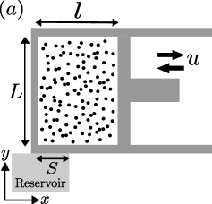
Figure 1: (a) Schematic illustration of a two-dimensional finite-time Carnot cycle model. Hard-disc particles as a weakly interacting nearly ideal gas are confined into the cylinder. The piston moves at a finite constant speed $u$ and the thermalizing wall with the length $S$ is set on the left bottom of the cylinder during the isothermal processes. (b) Temperature-volume ($T$-$V$) diagram of a quasistatic Carnot cycle for a two-dimensional ideal gas.

To mimic the weakly interacting nearly ideal gas, we confine a low dense $N$ hard-disc particles with diameter $d$ and mass $m$ into a cylinder with rectangular geometry and let them collide with each other. (Fig. 1 (a)) The head of the cylinder is a piston and it moves back and forth at a constant speed $u$. The usual quasistatic Carnot cycle ($u\to 0$) consists of four processes (Fig. 1 (b)): (A): isothermal expansion process ($V_{1}\to V_{2}$) in contact with the hot reservoir at the temperature $T_{\mathrm{h}}$, (B): adiabatic expansion process ($V_{2}\to V_{3}$), (C): isothermal compression process ($V_{3}\to V_{4}$) in contact with the cold reservoir at $T_{\mathrm{c}}$, (D): adiabatic compression process ($V_{4}\to V_{1}$), where $V_{k}$’s ($k=1,\cdots,4$) are the volumes of the cylinder at which we switch each of the four processes. $V_{k}$’s satisfy the relations $V_{3}=(T_{\mathrm{h}}/T_{\mathrm{c}})V_{2}$ and $V_{4}=(T_{\mathrm{h}}/T_{\mathrm{c}})V_{1}$ in the case of the two dimensional ideal gas. Since we regard our system of hard-disc particles as a nearly ideal gas, we apply these relations to our system. In the case of a finite-time cycle, we also switch each process at the same volume $V_{k}$ as in the quasistatic case.

Defining $(x,y)$ coordinates as in Fig. 1 (a), we let the piston move along the $x$-axis at a finite constant speed $u$. Here, we express the $x$-length and the $y$-length of the cylinder as $l$ and $L$, respectively and the volume of the cylinder as $V=Ll$. Then, the $x$-length $l_{k}$ at the switching volume $V_{k}$ can be defined as $l_{k}\equiv V_{k}/L$.

When a particle with the velocity $\mbox{\boldmath$v$}=(v_{x},v_{y})$ collides with the piston moving at the $x$-velocity $\pm u$, its velocity changes to $\mbox{\boldmath$v$}^{\prime}=(-v_{x}\pm 2u,v_{y})$, assuming perfectly elastic collision. Then the colliding particle gives the microscopic work $m(|\mbox{\boldmath$v$}|^{2}-|\mbox{\boldmath$v$}^{\prime}|^{2})/2=2m(\pm uv_{x}-u^{2})$ against the piston. In the isothermal processes (A) and (C), we set the thermalizing wall with the length $S$ at the position as in Fig. 1 (a). When a particle with the velocity $\mbox{\boldmath$v$}=(v_{x},v_{y})$ collides with the thermalizing wall, its velocity stochastically changes to the value governed by the distribution function

$$f(\mbox{\boldmath$v$},T_{i})=\frac{1}{\sqrt{2\pi}}\left(\frac{m}{k_{\mathrm{B}}T_{i}}\right)^{3/2}v_{y}\exp\left({-\frac{m\mbox{\boldmath$v$}^{2}}{2k_{\mathrm{B}}T_{i}}}\right)$$ (4)

($-\infty<v_{x}<+\infty,0<v_{y}<+\infty$, $T_{i}$ ($i=\mathrm{h}$ in (A), $\mathrm{c}$ in (C))), where $k_{\mathrm{B}}$ is the Boltzmann constant TTKB . The microscopic heat flowing from the thermalizing wall can be calculated by the difference between the kinetic energies before and after the collision. We sum up the above microscopic work and heat during one cycle. When $Q_{\mathrm{h}}$ denotes the heat flown from the hot reservoir during (A) and $Q_{\mathrm{c}}$ denotes the heat flown from the cold reservoir during (C), the total work $W$ during one cycle is expressed as $W\equiv Q_{\mathrm{h}}+Q_{\mathrm{c}}$. Then the power $P$ and the efficiency $\eta$ can be defined as $P\equiv\dot{W}$ and $\eta\equiv W/Q_{\mathrm{h}}\equiv P/\dot{Q}_{\mathrm{h}}$. Here, the dot denotes the value divided by one cycle period or the value per unit time throughout the paper. In our system, one cycle period is $2(l_{3}-l_{1})/u$.

III Molecular Kinetic Theory

In this section, we review the results of the molecular kinetic theory of the finite-time Carnot cycle obtained in our previous work. The details of the derivation of the equations in this section are described in IO .

If we assume that, even in a finite-time cycle, the gas relaxes to a uniform equilibrium state with a well-defined temperature $T$ sufficiently fast and the particle velocity $v$ is governed by Maxwell-Boltzmann distribution at $T$, we can easily derive the time-evolution equation of $T$ using the elementary molecular kinetic theory. Such an assumption of the fast relaxation to a uniform equilibrium state at a well-defined temperature $T$ is valid when the energy equilibration in the cylinder due to the inter-particle collisions is much faster than the speed of the energy transfers through the thermalizing wall and the piston. This situation is surely realized when $u$ is small and the interaction length $S$ between the gas and the reservoir is sufficiently small. If we assume that the gas is sufficiently close to a two-dimensional ideal gas, the internal energy of the gas can be approximated as $Nk_{\mathrm{B}}T$. Then, we can derive the time-evolution equation of the gas temperature $T$ for each of the four processes (A)-(D) as

$$\begin{array}[]{c c}(\mathrm{A}):Nk_{\mathrm{B}}\displaystyle{\frac{dT}{dt}}=q_{\mathrm{h}}-w_{\mathrm{e}},&(\mathrm{B}):Nk_{\mathrm{B}}\displaystyle{\frac{dT}{dt}}=-w_{\mathrm{e}},\\ \\ (\mathrm{C}):Nk_{\mathrm{B}}\displaystyle{\frac{dT}{dt}}=q_{\mathrm{c}}-w_{\mathrm{c}},&(\mathrm{D}):Nk_{\mathrm{B}}\displaystyle{\frac{dT}{dt}}=-w_{\mathrm{c}},\end{array}$$ (8)

where $q_{i}=q_{i}(t,T)$ ($i=\mathrm{h}$ in (A), $\mathrm{c}$ in (C)) is the heat flowing into the system per unit time in the isothermal processes and $w_{j}=w_{j}(t,T)$ ($j=\mathrm{e}$ in the expansion processes (A) and (B), $\mathrm{c}$ in the compression processes (C) and (D)) is the work against the piston per unit time. By counting the number of the particles colliding with the thermalizing wall and the piston, we can derive the specific forms of $q_{i}$ and $w_{\mathrm{e}}$ as

$$q_{i}(t,T)=\frac{3SNk_{\mathrm{B}}(T_{i}-T)}{4\pi V(t)}\sqrt{\frac{2\pi k_{\mathrm{B}}T}{m}},$$ (9)

$$w_{\mathrm{e}}(t,T) =\frac{2muNL}{V(t)}\biggl{\{}\frac{A^{2}T}{4}-A\sqrt{\frac{T}{\pi}}u+\frac{u^{2}}{2}$$ (10)

$$-\int_{0}^{\frac{u}{A\sqrt{T}}}d{v_{x}}\left(A\sqrt{T}{v_{x}}-u\right)^{2}\frac{\mathrm{e}^{-{v_{x}}^{2}}}{\sqrt{\pi}}\biggr{\}},$$

where $A\equiv\sqrt{{2k_{\mathrm{B}}}/{m}}$. $w_{\mathrm{c}}$ is also obtained by changing $u\to-u$ in Eq. (10).

Figure 2: Temperature-volume ($T$-$V$) diagram for the steady cycle obtained by numerically solving Eqs. (8) for $u=10^{-4}$ (dotted line) and $u=10^{-3}$ (dashed line). The solid line is a theoretical quasistatic Carnot cycle for a two-dimensional ideal gas. Since the dotted line is very close to the solid line, the case of $u=10^{-4}$ may be regarded as the quasistatic cycle. The parameters used are $N=100$, $T_{\mathrm{h}}=1$, $T_{\mathrm{c}}=0.7$, $S=0.05$, $m=1$, $k_{\mathrm{B}}=1$, $l_{1}=1$, $l_{2}=1.5$ and $L=1$.

We can numerically solve Eqs. (8) for the entire cycle at various piston speeds. By using the final temperature of each process as the initial temperature of the next process repeatedly, we can obtain a steady cycle at a given $u$. In Fig. 2, we have shown the temperature-volume ($T$-$V$) diagram for the steady cycle at $u=10^{-4}$ (dotted line) and $u=10^{-3}$ (dashed line), respectively. The solid line is the theoretical quasistatic line of a two-dimensional ideal gas. From this figure, we can see that as $u$ becomes larger, the cycle deviates from the theoretical quasistatic line and the temperatures during the isothermal processes (A) and (C) relax to the steady temperatures $T_{\mathrm{h}}^{\mathrm{st}}(<T_{\mathrm{h}})$ and $T_{\mathrm{c}}^{\mathrm{st}}(>T_{\mathrm{c}})$, respectively. If it is considered that the relaxation to the steady temperature is very fast, the isothermal process may approximately be divided into the relaxational part and the steady part in the case of a finite-time cycle, where $T(t)$ instantaneously changes from the initial temperature of the isothermal process to the steady temperature in the relaxational part and $T(t)$ keeps the steady temperature in the steady part. These relaxational parts in the isothermal processes (A) and (C) are surely missed in the original model by Curzon and Ahlborn CA ; IO ; BJM . Moreover we note that the heat flow per unit time $q_{i}$ as shown in Eq. (9) is time-dependent even during $T=T_{i}^{\mathrm{st}}$ through the volume of the cylinder after the relaxational processes in (A) and (C). Therefore the assumption of the time-independent heat flows in the original phenomenological model in CA does not seem to be applied to our model.

Although it may be impossible to find the exact solutions of Eqs. (8), we can find the analytic expressions of the steady temperature $T_{i}^{\mathrm{st}}$ during the isothermal processes (A) and (C) as the solutions of $dT/dt=0$ by expanding as $T_{i}^{\mathrm{st}}=T_{i}+a_{i}^{1}u+a_{i}^{2}u^{2}+O(u^{3})$, assuming that $u$ is small. These expansion coefficients $a_{i}^{1},a_{i}^{2}$, etc. can be determined order by order. If we assume that the relaxational process to $T_{\mathrm{h}}^{\mathrm{st}}$ is sufficiently fast, the heat $Q_{\mathrm{h}}^{\mathrm{st}}$ flowing into the system during the steady part $T(t)=T_{\mathrm{h}}^{\mathrm{st}}$ can be calculated up to $O(u)$ as:

$$Q_{\mathrm{h}}^{\mathrm{st}} =\int_{0}^{(l_{2}-l_{1})/u}q_{\mathrm{h}}(t,T_{\mathrm{h}}^{\mathrm{st}})\ dt$$ (11)

$$=Q_{\mathrm{h}}^{\mathrm{qs}}-2mNA\sqrt{T_{\mathrm{h}}\pi}\left(\frac{1}{\pi}+\frac{L}{3S}\right)u\ln\frac{V_{2}}{V_{1}},$$

where the quasistatic heat for an ideal gas in the isothermal process (A) is defined as $Q_{\mathrm{h}}^{\mathrm{qs}}=Nk_{\mathrm{B}}T_{\mathrm{h}}\ln(V_{2}/V_{1})$. $Q_{\mathrm{c}}^{\mathrm{st}}$ during $T(t)=T_{\mathrm{c}}^{\mathrm{st}}$ can also be obtained by changing $u\to-u$, $T_{\mathrm{h}}\to T_{\mathrm{c}}$ and $V_{2}/V_{1}\to V_{4}/V_{3}$ in Eq. (11). If we neglect the contributions of the heat transfers through the thermalizing wall during the relaxational parts in (A) and (C), the steady part of the work during one cycle $W^{\mathrm{st}}\equiv Q_{\mathrm{h}}^{\mathrm{st}}+Q_{\mathrm{c}}^{\mathrm{st}}$ becomes

$$W^{\mathrm{st}} =Nk_{\mathrm{B}}(T_{\mathrm{h}}-T_{\mathrm{c}})\ln\frac{V_{2}}{V_{1}}-2mNA\sqrt{\pi}\left(\frac{1}{\pi}+\frac{L}{3S}\right)$$ (12)

$$\times(\sqrt{T_{\mathrm{h}}}+\sqrt{T_{\mathrm{c}}})u\ln\frac{V_{2}}{V_{1}}.$$

If we assume that the adiabatic processes (B) and (D) even at a finite $u$ satisfy the quasistatic adiabatic relation $TV=\mathrm{const}$ of a two-dimensional ideal gas, the additional heat transfers $Q_{\mathrm{h}}^{\mathrm{add}}$ and $Q_{\mathrm{c}}^{\mathrm{add}}$ during the relaxational part in (A) and (C), respectively, can be estimated as

$$Q_{\mathrm{h}}^{\mathrm{add}}=-Nk_{\mathrm{B}}\frac{4L\sqrt{\pi T_{\mathrm{h}}}}{3SA}\left(1+\sqrt{\frac{T_{\mathrm{h}}}{T_{\mathrm{c}}}}\right)u$$ (13)

up to $O(u)$ and $Q_{\mathrm{c}}^{\mathrm{add}}$ can also be obtained by changing $u\to-u$ and $T_{\mathrm{h}}\leftrightarrow T_{\mathrm{c}}$ in Eq. (13). Therefore the total $Q_{\mathrm{h}}$, $Q_{\mathrm{c}}$ and $W$ become $Q_{\mathrm{h}}=Q_{\mathrm{h}}^{\mathrm{st}}+Q_{\mathrm{h}}^{\mathrm{add}}$, $Q_{\mathrm{c}}=Q_{\mathrm{c}}^{\mathrm{st}}+Q_{\mathrm{c}}^{\mathrm{add}}$ and $W=W^{\mathrm{st}}+Q_{\mathrm{h}}^{\mathrm{add}}+Q_{\mathrm{c}}^{\mathrm{add}}$, respectively.

IV Calculation of Onsager coefficients

After the preliminaries in the previous sections, we can now calculate the Onsager coefficients for our finite-time Carnot cycle in the linear-response regime $\Delta T\to 0$ as follows. The first step is an appropriate choice of the thermodynamic forces and fluxes for this system. A typical way to choose these thermodynamic forces and fluxes is to introduce the rate of the total entropy production $\dot{\sigma}$ during one cycle:

$$\dot{\sigma}\equiv-\frac{\dot{Q}_{\mathrm{h}}}{T_{\mathrm{h}}}-\frac{\dot{Q}_{\mathrm{c}}}{T_{\mathrm{c}}}.$$ (14)

This is just the entropy increase of the two reservoirs during one cycle divided by the cycle period $2(l_{3}-l_{1})/u$ because the entropy of the working substance does not change after one cycle. Using the relation $Q_{\mathrm{c}}=W-Q_{\mathrm{h}}$ and considering the linear-response regime $\Delta T\to 0$, it can be rewritten as

$$\dot{\sigma}=\frac{u(-W)}{2(l_{3}-l_{1})T}+\frac{\Delta T}{T^{2}}\dot{Q}_{\mathrm{h}},$$ (15)

where $T\equiv(T_{\mathrm{h}}+T_{\mathrm{c}})/2$ and we have neglected ${\Delta T}^{3}\dot{Q}_{\mathrm{h}}$ and $uW\Delta T$ terms, the reason of which we will clarify later. According to the linear-response theory, $\dot{\sigma}$ can be expressed as the sum of the product of the thermodynamic force and its conjugate thermodynamic flux O ; GM :

$$\dot{\sigma}=J_{1}X_{1}+J_{2}X_{2},$$ (16)

where we define the thermodynamic forces as

$$X_{1}\equiv\frac{-W}{2(l_{3}-l_{1})T},\ X_{2}\equiv\frac{\Delta T}{T^{2}}$$ (17)

and their conjugate fluxes as

$$J_{1}\equiv u,\ J_{2}\equiv\dot{Q}_{\mathrm{h}}.$$ (18)

Moreover the linear-response theory assumes the Onsager relations between the fluxes and forces O ; GM :

$$J_{1} =u=L_{11}\frac{-W}{2(l_{3}-l_{1})T}+L_{12}\frac{\Delta T}{T^{2}},$$ (19)

$$J_{2} =\dot{Q}_{\mathrm{h}}=L_{21}\frac{-W}{2(l_{3}-l_{1})T}+L_{22}\frac{\Delta T}{T^{2}},$$ (20)

where $L_{ij}$’s are the Onsager coefficients and the non-diagonal elements should satisfy the symmetry relation $L_{12}=L_{21}$. From these relations between the thermodynamic fluxes and forces, we understand that $\dot{\sigma}=J_{1}X_{1}+J_{2}X_{2}$ is the quantity of the second-order of the thermodynamic forces, which explain why we neglected the higher order terms like ${\Delta T}^{3}\dot{Q}_{\mathrm{h}}$ and $uW\Delta T$ in Eq. (15). Moreover, although we considered the contributions of the additional heat transfers $Q_{\mathrm{h}}^{\mathrm{add}}$ and $Q_{\mathrm{c}}^{\mathrm{add}}$ to the total heat and the work in Sec. III, we can easily show that their effects do not contribute to $\dot{\sigma}$ in the limit of $\Delta T\to 0$. Therefore we can indeed neglect them in the linear-response regime and use $Q_{\mathrm{h}}=Q_{\mathrm{h}}^{\mathrm{st}}$ and $W=W^{\mathrm{st}}$ in the calculations of the Onsager coefficients below.

We are now in a position to calculate the Onsager coefficients explicitly. First we determine $L_{11}$ and $L_{21}$ as follows. To calculate $L_{11}$, we consider the relation between $u$ and $X_{1}$ in the case of $\Delta T=0$. Expanding Eq. (12) by $\Delta T$ and putting $\Delta T=0$, we can obtain the relation

$$W=-4mNA\sqrt{\pi T}\left(\frac{1}{\pi}+\frac{L}{3S}\right)\ln\frac{V_{2}}{V_{1}}\times u.$$ (21)

Comparing Eq. (21) with Eq. (19), $L_{11}$ is determined as

$$L_{11}=\frac{(l_{3}-l_{1})T^{1/2}}{2mN(\frac{1}{\pi}+\frac{L}{3S})\sqrt{\frac{2\pi k_{\mathrm{B}}}{m}}\ln\frac{V_{2}}{V_{1}}}.$$ (22)

Likewise $\dot{Q}_{\mathrm{h}}$ with $\Delta T=0$ can be evaluated up to the linear order in $W$ using Eq. (11) and (21) as

$$\dot{Q}_{\mathrm{h}}=\frac{k_{\mathrm{B}}T^{3/2}}{4m(\frac{1}{\pi}+\frac{L}{3S})\sqrt{\frac{2\pi k_{\mathrm{B}}}{m}}}\frac{-W}{2(l_{3}-l_{1})T}.$$ (23)

Comparing Eq. (23) with Eq. (20), $L_{21}$ is determined as

$$L_{21}=\frac{k_{\mathrm{B}}T^{3/2}}{4m(\frac{1}{\pi}+\frac{L}{3S})\sqrt{\frac{2\pi k_{\mathrm{B}}}{m}}}.$$ (24)

Next we determine $L_{12}$ and $L_{22}$ as follows. To calculate $L_{12}$, we consider the relation between $u$ and $X_{2}$ in the case of $W=0$. In this case, regardless of a finite temperature difference, useful work cannot be obtained because the engine runs so fast that it cannot output positive work. Therefore, this case is called the work-consuming state. The speed of the piston at the work-consuming state can be obtained as a solution of $W=0$ in Eq. (12). Considering in the linear-response regime $\sqrt{T_{\mathrm{h}}}-\sqrt{T_{\mathrm{c}}}\simeq\Delta T/(2\sqrt{T})$, it becomes

$$u =\frac{k_{\mathrm{B}}T^{3/2}}{4m(\frac{1}{\pi}+\frac{L}{3S})\sqrt{\frac{2\pi k_{\mathrm{B}}}{m}}}\frac{\Delta T}{T^{2}}.$$ (25)

From Eq. (19) and Eq. (25), we can obtain

$$L_{12}=\frac{k_{\mathrm{B}}T^{3/2}}{4m(\frac{1}{\pi}+\frac{L}{3S})\sqrt{\frac{2\pi k_{\mathrm{B}}}{m}}}.$$ (26)

From Eqs. (24) and (26), we can confirm the symmetry relation $L_{12}=L_{21}$ as expected. To determine the last coefficient $L_{22}$, we consider the heat flow $\dot{Q}_{\mathrm{h}}$ at the work-consuming state using Eq. (11) and (25):

$$\dot{Q}_{\mathrm{h}}=\frac{Nk_{\mathrm{B}}^{2}\ln\frac{V_{2}}{V_{1}}}{8m(\frac{1}{\pi}+\frac{L}{3S})\sqrt{\frac{2\pi_{\mathrm{B}}}{m}}(l_{3}-l_{1})}T^{5/2}\frac{\Delta T}{T^{2}}.$$ (27)

From Eq. (20) and Eq. (27), the last coefficient $L_{22}$ turns out to be

$$L_{22}=\frac{Nk_{\mathrm{B}}^{2}\ln\frac{V_{2}}{V_{1}}T^{5/2}}{8m(\frac{1}{\pi}+\frac{L}{3S})\sqrt{\frac{2\pi_{\mathrm{B}}}{m}}(l_{3}-l_{1})}.$$ (28)

Note that the positivity of the rate of the total entropy production, $\dot{\sigma}=J_{1}X_{1}+J_{2}X_{2}\geq 0$, should restrict the values of the Onsager coefficients to $L_{11}\geq 0$, $L_{22}\geq 0$ and $L_{11}L_{22}-L_{12}L_{21}\geq 0$. We can confirm that $L_{ij}$ of our finite-time Carnot cycle surely satisfy these relations. These analytic expressions of the Onsager coefficients $L_{ij}$ are the main result of this paper.

To confirm the validity of the above analytic calculations of the Onsager coefficients, especially $T$ dependence of them, we performed the event-driven molecular dynamics (MD) computer simulations IO ; IO2 ; AW of our two-dimensional finite-time Carnot cycle, following the procedure described in Sec. II.

To calculate $L_{12}$ and $L_{22}$ at given $T$, we fix the temperature difference $\Delta T$ to a sufficiently small value and find the piston speed where the work becomes $0$. Then we can determine $L_{12}$ and $L_{22}$ numerically as

$$L_{12} =\frac{J_{1}}{X_{2}}=\frac{uT^{2}}{\Delta T},$$ (29)

$$L_{22} =\frac{J_{2}}{X_{2}}=\frac{\dot{Q}_{\mathrm{h}}T^{2}}{\Delta T}$$ (30)

from Eq. (19) and Eq. (20). Next, to calculate $L_{11}$ and $L_{21}$ at given $T$, we set $\Delta T=0$. Fixing $u$ to a sufficiently small value ($2.5\times 10^{-5}\sim 3\times 10^{-4}$), we can determine $L_{11}$ and $L_{21}$ numerically as

$$L_{11} =\frac{J_{1}}{X_{1}}=-\frac{2(l_{3}-l_{1})Tu}{W},$$ (31)

$$L_{21} =\frac{J_{2}}{X_{1}}=-\frac{2(l_{3}-l_{1})T\dot{Q}_{\mathrm{h}}}{W}$$ (32)

from using Eq. (19) and Eq. (20). Fig. 3 shows $T$ dependence of these Onsager coefficients determined by the MD simulations as well as the analytic results. We can see fairly good agreement between the MD data and the analytic lines in the range we studied. These data clearly support the validity of our analytic expressions of the Onsager coefficients which has been obtained under some theoretical assumptions.

Figure 3: $T$-dependence of the Onsager coefficients. The dashed line, the solid line and the dotted line indicate the theoretical Onsager coefficient $L_{22}$ (Eq. (28)), $L_{12}$ (Eq. (26)) ($=L_{21}$ (Eq. (24))) and $L_{11}$ (Eq. (22)), respectively. The parameters used in the MD simulations are $\Delta T=4\times 10^{-3}$ and $d=0.01$. The other parameters are the same as in Fig. 2. The MD data were obtained by averaging $100$-$800$ cycles after transient $5$ cycles in the simulations.

V The efficiency at the maximal power

To see how the Onsager coefficients derived in Sec. IV indeed govern the behavior of the finite-time Carnot cycle, we briefly introduce the general framework of the heat engine obeying the Onsager relations VB .

The basic setup is as follows. We consider a general steady or cyclic process in which the work is extracted from the heat flow between the small temperature difference. (see Fig. 4)

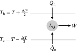
Figure 4: Schematic illustration of the heat engine governed by the Onsager relations Eq. (33) and Eq. (34).

The work $W$ done against the external force $F$ is $W=-Fx$ where $x$ is the thermodynamically conjugate variable of $F$. We define a thermodynamic force as $X_{1}=F/T$ and the corresponding thermodynamic flux as $J_{1}=\dot{x}$. We also choose $X_{2}=1/T_{\mathrm{c}}-1/T_{\mathrm{h}}$ as another thermodynamic force and $J_{2}=\dot{Q}_{\mathrm{h}}$ as the corresponding thermodynamic flux. If we consider the linear-response regime $\Delta T\to 0$, $X_{2}$ can be written as $X_{2}\simeq\Delta T/T^{2}$. Moreover the linear-response theory assumes the Onsager relations between the thermodynamic forces and fluxes O ; GM :

$$J_{1} =L_{11}X_{1}+L_{12}X_{2},$$ (33)

$$J_{2} =L_{21}X_{1}+L_{22}X_{2},$$ (34)

where the non-diagonal elements of the Onsager coefficients should satisfy $L_{12}=L_{21}$. Then, the power $P=\dot{W}$ and the efficiency $\eta=P/\dot{Q}_{\mathrm{h}}$ of the engine can be expressed as

$$P =-J_{1}X_{1}T,$$ (35)

$$\eta =\frac{-J_{1}X_{1}T}{J_{2}}.$$ (36)

Now the efficiency at the maximal power $\eta_{\mathrm{max}}$ can be given as follows: We first maximize the power at $X_{1}=-L_{12}X_{2}/(2L_{11})$ which is determined as the solution of $\partial P/\partial X_{1}=0$, then, $\eta_{\mathrm{max}}$ becomes

$$\eta_{\mathrm{max}}=\frac{\Delta T}{2T}\frac{q^{2}}{2-q^{2}},$$ (37)

where

$$q\equiv\frac{L_{12}}{\sqrt{L_{11}L_{22}}}$$ (38)

is called the coupling strength parameter. Note that it takes $-1\leq q\leq+1$ due to the positivity of $\dot{\sigma}$. When $q$ satisfies the tight-coupling condition $|q|=1$, $\eta_{\mathrm{max}}$ takes the maximal value $\Delta T/(2T)$, which is equal to the CA efficiency up to the lowest order in $\Delta T$.

In Refs. IO ; IO2 , we studied $\eta_{\mathrm{max}}$ of this finite-time Carnot cycle extensively by performing the MD computer simulations as a numerical experiment to verify the validity of the CA efficiency. We found there that $\eta_{\mathrm{max}}$ agrees with the CA efficiency in the limit of $\Delta T\to 0$. Our molecular kinetic theory also confirmed this property IO : Using $Q_{i}=Q_{i}^{\mathrm{st}}+Q_{i}^{\mathrm{add}}$ in Sec. III, we can calculate the speed $u=u_{\mathrm{max}}$ at which the power $P$ maximizes as

$$u_{\mathrm{max}} =\frac{k_{\mathrm{B}}(T_{\mathrm{h}}-T_{\mathrm{c}})}{\sqrt{\pi}}\Biggl{\{}4mA\left(\frac{L}{3S}+\frac{1}{\pi}\right)$$ (39)

$$\times(\sqrt{T_{\mathrm{h}}}+\sqrt{T_{\mathrm{c}}})\ln\frac{V_{2}}{V_{1}}+\frac{8Lk_{\mathrm{B}}}{3SA\sqrt{T_{\mathrm{h}}}}$$

$$\times\left(T_{\mathrm{h}}-T_{\mathrm{c}}\right)\left(1+\sqrt{\frac{T_{\mathrm{h}}}{T_{\mathrm{c}}}}\right)\Biggr{\}}^{-1}\ln\frac{V_{2}}{V_{1}},$$

and can confirm that the efficiency $\eta$ at $u=u_{\mathrm{max}}$ shows

$$\eta_{\mathrm{max}}\equiv\eta(u_{\mathrm{max}}) =\frac{W(u_{\mathrm{max}})}{Q_{\mathrm{h}}^{\mathrm{st}}(u_{\mathrm{max}})+Q_{\mathrm{h}}^{\mathrm{add}}(u_{\mathrm{max}})}$$ (40)

$$\to\frac{\Delta T}{2T}\ (\Delta T\to 0).$$

Now we can clarify the underlying physics of this behavior of $\eta_{\mathrm{max}}$. In the limit of $\Delta T\to 0$, our finite-time Carnot cycle can be described by the Onsager relations as shown in Sec IV. Then we can confirm that $q=1$ in our finite-time Carnot cycle from Eqs. (22), (26), (28) and (38). This condition gives a proof that our finite-time Carnot cycle shows the CA efficiency in the limit of $\Delta T\to 0$ as suggested in IO ; IO2 from the viewpoint of the linear-response theory.

VI Summary

In this paper, we have studied a finite-time Carnot cycle of a two-dimensional weakly interacting nearly ideal gas working in the linear-response regime and have explicitly calculated the Onsager coefficients of this system for the first time. Molecular dynamics computer simulations of this cycle have supported the theoretical calculations in spite of some assumptions in the analysis. We have revealed that the Onsager coefficients of this system satisfy the tight-coupling condition $q=L_{12}/\sqrt{L_{11}L_{22}}=1$ and therefore can understand why our finite-time Carnot cycle attains the Curzon-Ahlborn efficiency in the linear-response regime $\Delta T\to 0$ as suggested in Refs. IO ; IO2 . It would be an interesting problem to construct and study the collective behavior of the Carnot cycles coupled with each other by using the property of the Onsager coefficients derived in this paper OAMB ; VB ; VB2 ; JA ; JA2 .

- (1) F. Curzon and B. Ahlborn, Am. J. Phys. 43, 22 (1975).
- (2) H. Callen, Thermodynamics and an Introduction to Thermostatistics (Wiley, New York, 1985), 2nd ed, Chap. 4.
- (3) I. I. Novikov, J. Nuclear Energy II 7, 125 (1958).
- (4) Y. Izumida and K. Okuda, Europhys. Lett. 83, 60003 (2008).
- (5) Y. Izumida and K. Okuda, Prog. Theor. Phys. Suppl. 178, 163-168 (2009).
- (6) C. Van den Broeck, Phys. Rev. Lett. 95, 190602 (2005).
- (7) A. Gomez-Marin and J. M. Sancho, Phys. Rev. E 74, (062102) (2006).
- (8) T. Schmiedl and U. Seifert, Europhys. Lett. 81, 20003 (2008).
- (9) Z. C. Tu, J. Phys. A. 41, 312003 (2008).
- (10) M. Esposito, K. Lindenberg, and C. Van den Broeck, Europhys. Lett. 85, 60010 (2009).
- (11) M. Esposito, K. Lindenberg, and C. Van den Broeck, Phys. Rev. Lett. 102, 130602 (2009).
- (12) R. Benjamin and R. Kawai, Phys. Rev. E 77, 051132 (2008).
- (13) R. Tehver, F. Toigo, J. Koplik, and J. R. Banavar, Phys. Rev. E 57, R17 (1998).
- (14) J. Birjukov, T. Jahnke and G. Mahler, Euro. Phys. J. B, 64, 105 (2008).
- (15) L. Onsager, Phys. Rev. 37, 405 (1931).
- (16) S. R. de Groot and P. Mazur, Non-Equilibrium Thermodynamics (Dover, New York, 1984).
- (17) B. J. Alder and T. E. Wainwright, J. Chem. Phys. 31, 459 (1959).
- (18) M. J. Ondrechen, B. Andresen, M. Mozurkewich, and R. S. Berry, Am. J. Phys. 49, 681 (1981).
- (19) C. Van den Broeck, Adv. Chem. Phys. 135, 189 (2007).
- (20) B. Jiménez de Cisneros and A. Calvo Hernández, Phys. Rev. Lett. 98, 130602 (2007).
- (21) B. Jiménez de Cisneros and A. Calvo Hernández, Phys. Rev. E 77, 041127 (2008).