A Fast Parallel Poisson Solver on Irregular Domains Applied to Beam Dynamic Simulations

Abstract

We discuss the scalable parallel solution of the Poisson equation within a Particle-In-Cell (PIC) code for the simulation of electron beams in particle accelerators of irregular shape. The problem is discretized by Finite Differences. Depending on the treatment of the Dirichlet boundary the resulting system of equations is symmetric or ‘mildly’ nonsymmetric positive definite. In all cases, the system is solved by the preconditioned conjugate gradient algorithm with smoothed aggregation (SA) based algebraic multigrid (AMG) preconditioning. We investigate variants of the implementation of SA-AMG that lead to considerable improvements in the execution times. We demonstrate good scalability of the solver on distributed memory parallel processor with up to 2048 processors. We also compare our SAAMG-PCG solver with an FFT-based solver that is more commonly used for applications in beam dynamics.

1 Introduction

In recent years, precise beam dynamics simulations in the design of high-current low-energy hadron machines as well as of 4th generation light sources have become a very important research topic. Hadron machines are characterized by high currents and hence require excellent control of beam losses and/or keeping the emittance (a measure of the phase space) of the beam in narrow ranges. This is a challenging problem which requires the accurate modeling of the dynamics of a large ensemble of macro or real particles subject to complicated external focusing, accelerating and wake-fields, as well as the self-fields caused by the Coulomb interaction of the particles. In general the geometries of particle accelerators are large and complicated. The discretization of the computational domain is time dependent due to the relativistic nature of the problem. time and space dilatation. Both phenomenas have a direct impact on the numerical solution method.

The solver described in this paper is part of a general accelerator modeling tool OPAL (Object Oriented Parallel Accelerator Library) [2]. OPAL allows to tackle the most challenging problems in the field of high precision particle accelerator modeling. These include the simulation of high power hadron accelerators and of next generation light sources.

Some of the effects can be studied by using a low dimensional model, i.e., envelope equations [21, 22, 27, 6]. These are a set of ordinary differential equations for the second-order moments of a time-dependent particle distribution. They can be calculated fast, however the level of detail is mostly insufficient for quantitative studies. Furthermore, a priori knowledge of critical beam parameters such as the emittance is required with the consequence that the envelope equations cannot be used as a self-consistent method.

One way to overcome these limitations is by considering the Vlasov-Poisson description of the phase space, including external and self-fields and, if needed, other effects such as wakes. To that end let $f(\mathbf{x},\mathbf{v},t)$ be the density of the particles in the phase space, i.e., the position-velocity $(\mathbf{x},\mathbf{v})$ space. Its evolution is determined by the collisionless Vlasov equation,

$$\frac{df}{dt}=\partial_{t}f+\mathbf{v}\cdot\nabla_{\mathbf{x}}f+\frac{q}{m_{0}}(\mathbf{E}+\mathbf{v}\times\mathbf{B})\cdot\nabla_{\mathbf{v}}f=0,$$ (1)

where $m_{0}$, $q$ denote particle mass and charge, respectively. The electric and magnetic fields $\mathbf{E}$ and $\mathbf{B}$ are superpositions of external fields and self-fields (space charge),

$$\mathbf{E}=\mathbf{E_{\mathrm{ext}}}+\mathbf{E_{\mathrm{self}}},\quad\mathbf{B}=\mathbf{B_{\mathrm{ext}}}+\mathbf{B_{\mathrm{self}}}.$$ (2)

If $\mathbf{E}$ and $\mathbf{B}$ are known, then each particle can be propagated according to the equation of motion for charged particles in an electromagnetic field,

$$\frac{d\mathbf{x}(t)}{dt}=\mathbf{v},\quad\frac{d\mathbf{v}(t)}{dt}=\frac{q}{m_{0}}\left(\mathbf{E}+\mathbf{v}\times\mathbf{B}\right).$$

After the movement of the particles $\mathbf{E_{\mathrm{self}}}$ and $\mathbf{B_{\mathrm{self}}}$ have to be updated. To that end we change the coordinate system into the one moving with the particles. By means of the appropriate Lorentz transformation [15] we arrive at a (quasi-) static approximation of the system in which the transformed magnetic field becomes negligible, $\hat{\mathbf{B}}\!\approx\!\mathbf{0}$. The transformed electric field is obtained from

$$\hat{\mathbf{E}}=\hat{\mathbf{E}}_{\mathrm{self}}=-\nabla\hat{\phi},$$ (3)

where the electrostatic potential $\hat{\phi}$ is the solution of the Poisson problem

$$-\Delta\hat{\phi}(\mathbf{x})=\frac{\hat{\rho}(\mathbf{x})}{\varepsilon_{0}},$$ (4)

equipped with appropriate boundary conditions, see section 2. Here, $\hat{\rho}$ denotes the spatial charge density and $\varepsilon_{0}$ is the dielectric constant. By means of the inverse Lorentz transformation the electric field $\hat{\mathbf{E}}$ can then be transformed back to yield both the electric and the magnetic fields in (2).

The Poisson problem (4) discretized by finite differences can efficiently be solved on a rectangular grid by a Particle-In-Cell (PIC) approach [20]. The right hand side in (4) is discretized by sampling the particles at the grid points. In (3), $\hat{\phi}$ is interpolated at the particle positions from its values at the grid points. We also note that the FFT-based Poisson solvers and similar approaches [20, 19] are restricted to box-shaped or open domains.

Serafini et al. [24] report on a state-of-the-art conventional FFT-based algorithm for solving the Poisson equation with ‘infinite-domain’, i.e., open boundary conditions for large problems in accelerator modeling. The authors show improvements in both accuracy and performance, by combining several techniques: the method of local corrections, the James algorithm, and adaptive mesh refinement.

However with the quest of high intensity, high brightness beams together with ultra low particle losses, there is a high demand to consider the true geometry of the beam-pipe in the numerical model. This assures that the image charge components are taken properly into account. This results in a more exact modeling of the non-linear beam dynamics which is indispensable for the next generation of particle accelerators.

In a related paper by Pöplau et al. [18], an iterative solver preconditioned by geometric multigrid is used to calculate space-charge forces. The authors employ a mesh with adaptive spacings to reduce the workload of the BiCGStab solver used to solve the nonsymmetric system arising from quadratic extrapolation at the boundary. The geometric multigrid solver used in their approach is much more sensitive to anisotropic grids arising in beam dynamic simulations (e.g. special coarsening operators have to be defined). With smoothed aggregation-based algebraic multigrid (AMG) preconditioning as used in this paper the aggregation smoother takes care of anisotropies and related issues and leads to a robustness superior to geometric multigrid, see [30] for a discussion. The preconditioner easily adapts to the elongation of the computational domain that happens during our simulation.

In Section 2 we describe how the Poisson equation on a ‘general’ domain $\Omega\subset\mathbb{R}^{3}$ can be solved by finite differences and the PIC approach. We treat the boundary in three different ways, by constant, by linear, and by quadratic extrapolation, the latter being similar to the approach of McCorquodale et al. [17]. The system of equation is solved by the conjugate gradient algorithm preconditioned by smoothed aggregation AMG [33, 32], see Section 3. For this solver we coined the acronym: SAAMG-PCG. The preconditioned conjugate gradient (PCG) algorithm is also used if the system is ‘mildly’ nonsymmetric. In Section 4 we deal with details of the implementation, in particular its parallelization. In Section 5 we report on numerical experiments including a physical application from beam dynamics. In Section 6 we draw our conclusions.

2 The discretization

In this section we discuss the solution of the Poisson equation in a domain

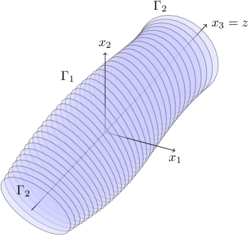
Figure 1: Sketch of a typical domain

$\Omega\subset\mathbb{R}^{3}$ as indicated in Figure 1. The boundary of the domain is composed of two parts, a curved, smooth surface $\Gamma_{1}$ and two planar portions at $z=-d$ and $z=+d$ that form together $\Gamma_{2}$. In physical terms $\Gamma_{1}$ forms the casing of the pipe, while $\Gamma_{2}$ is the open boundary at the inlet and outlet of the beam pipe, respectively. The centroid of the particle bunch is at the origin of the coordinate system. The Poisson problem that we are going to solve is given by

$$-\Delta\phi =\frac{\rho}{\epsilon_{0}}\ \text{in}\ \Omega,$$ (5)

$$\phi =g\equiv 0\ \text{on}\ \Gamma_{1},$$

$$\frac{\partial\phi}{\partial\mathbf{n}}+\frac{1}{d}\phi =0\ \text{on}\ \Gamma_{2}.$$

The parameter $d$ in the Robin boundary condition denotes the distance of the charged particles to the boundary [18]. It is half the extent of $\Omega$ in $z$-direction. Notice that the Robin boundary condition applies only on the planar paraxial portions of the boundary.

We discretize (5) by a second order finite difference scheme defined on a rectangular lattice (grid)

$$\Omega_{h}:=\left\{\mathbf{x}\in{\Omega}\cup\Gamma_{2}\ |\ x_{i}/h_{i}\in\mathbb{Z}\ \mbox{for}\ i=1,2,3\right\},$$

where $h_{i}$ is the grid spacing and $\mathbf{e}_{i}$ the unit vector in the $i$-th coordinate direction. The grid is arranged in a way that the two portions of $\Gamma_{2}$ lie in grid planes. A lattice point is called an interior point if all its direct neighbours are in $\Omega$. All other grid points are called near-boundary points. At interior points $\mathbf{x}$ we approximate $\Delta u(\mathbf{x})$ by the well-known 7-point difference star

$$-\Delta_{h}u(\mathbf{x})=\sum_{i=1}^{3}\frac{-u(\mathbf{x}\!-\!h_{i}\mathbf{e}_{i})+2u(\mathbf{x})-u(\mathbf{x}\!+\!h_{i}\mathbf{e}_{i})}{h_{i}^{2}}.$$ (6)

At grid points near the boundary we have to take the boundary conditions in (5) into account. To explain the schemes on the Dirichlet (or PEC) boundary $\Gamma_{1}$ let $\mathbf{x}$ be a near-boundary point. Let $\mathbf{x}^{\prime}:=\mathbf{x}-h_{i}\mathbf{e}_{i}$ for some $i$ be outside $\Omega$ and let $\mathbf{x}^{*}:=\mathbf{x}-sh_{i}\mathbf{e}_{i}$, $0<s\leq 1$, be the boundary point between $\mathbf{x}$ and $\mathbf{x}^{\prime}$ that is closest to $\mathbf{x}$, cf. Figure 2.

Figure 2: 1-dimensional sketch of a near-boundary point $x$

If $s=1$, i.e., if $\mathbf{x}^{\prime}\in\partial\Omega$ then $u(\mathbf{x}^{\prime})$ in (6) is replaced by the prescribed boundary value. Otherwise, we proceed in one of the three following ways [5, 10]

1. In constant extrapolation the boundary value prescribed at $\mathbf{x}-sh_{i}\mathbf{e}_{i}\in\Gamma_{1}$ is assigned to $u(\mathbf{x}^{\prime})$,

   $$u(\mathbf{x}^{\prime})=u(\mathbf{x}-h_{i}\mathbf{e}_{i}):=g(\mathbf{x}^{*}).$$ (7)

2. In linear extrapolation the value at $\mathbf{x}^{\prime}$ is obtained by means of the values $u$ at $\mathbf{x}$ and at $\mathbf{x}-sh_{i}\mathbf{e}_{i}$,

   $$u(\mathbf{x}^{\prime}):=(1-\frac{1}{s})\,u(\mathbf{x})+\frac{1}{s}\,g(\mathbf{x}^{*}).$$ (8)

3. Quadratic extrapolation amounts to the Shortley-Weller approximation [5, 26, 17]. If $\mathbf{x}^{\prime\prime}:=\mathbf{x}+h_{i}\mathbf{e}_{i}\in\Omega_{h}$ then the value $u(\mathbf{x}^{\prime})$ is obtained by quadratic interpolation of the values of $u$ at $\mathbf{x}$, $\mathbf{x}^{\prime\prime}$, and the boundary point $\mathbf{x}^{*}$,

   $$u(\mathbf{x}^{\prime}):=\frac{2(s\!-\!1)}{s}u(\mathbf{x})-\frac{s\!-\!1}{s\!+\!1}u(\mathbf{x^{\prime\prime}})+\frac{2}{s(s\!+\!1)}g(\mathbf{x}^{*}).$$ (9)

   If $\mathbf{x}^{\prime\prime}\not\in\Omega_{h}$ then let $\mathbf{x}^{**}:=\mathbf{x}+th_{i}\mathbf{e}_{i}$, $0<t\leq 1$, be the boundary point between $\mathbf{x}$ and $\mathbf{x}^{\prime\prime}$ that is closest to $\mathbf{x}$. Then, similarly as before, we get

   $$u(\mathbf{x}^{\prime}) :=\frac{(s\!-\!1)(t\!+\!1)}{st}u(\mathbf{x})+\frac{(t\!+\!1)}{(s\!+\!t)s}g(\mathbf{x}^{*})-\frac{(s\!-\!1)}{(s\!+\!t)t}g(\mathbf{x}^{**}),$$ (10)

   $$u(\mathbf{x}^{\prime\prime}) :=\frac{(s\!+\!1)(t\!-\!1)}{st}u(\mathbf{x})-\frac{(t\!-\!1)}{(s\!+\!t)s}g(\mathbf{x}^{*})+\frac{(s\!+\!1)}{(s\!+\!t)t}g(\mathbf{x}^{**}).$$

In all extrapolation formulae given above we set $g(\mathbf{x}^{*})=g(\mathbf{x}^{**})=0$ according to (5). The value on the right side of (7)–(10) substitutes $u(\mathbf{x}\!\pm\!h_{i}\mathbf{e}_{i})$ in (6).

Let us now look at a grid point $\mathbf{x}$ on the open boundary $\Gamma_{2}$. If $\mathbf{x}$ is located on the inlet of the beam pipe then $\mathbf{x}^{\prime\prime}:=\mathbf{x}\!+\!h_{3}\mathbf{e}_{3}\in\Omega$ and $\mathbf{x}^{\prime}:=\mathbf{x}\!-\!h_{3}\mathbf{e}_{3}\not\in\Omega$. The Robin boundary condition is approximated by a central difference,

$$-\frac{u(\mathbf{x}^{\prime\prime})-u(\mathbf{x}^{\prime})}{2h_{3}}+\frac{1}{d}u(\mathbf{x})=0,$$

or

$$u(\mathbf{x}^{\prime})=u(\mathbf{x}^{\prime\prime})-\frac{2h_{3}}{d}u(\mathbf{x}).$$ (11)

The same formula holds on the outlet boundary portion if $\mathbf{x}^{\prime}$ denotes the virtual grid point outside $\Omega$.

Notice that some lattice points may be close to the boundary with regard to more than one coordinate direction. Then, the procedures (7)–(11) must be applied to all of them.

The finite difference discretization just described leads to a system of equations

$$A\mathbf{x}=\mathbf{b},$$ (12)

where $\mathbf{x}$ is the vector of unknown values of the potential and $\mathbf{b}$ is the vector of the charge density interpolated at the grid points. The Poisson matrix $A$ is an $M$-matrix irrespective of the boundary treatment [10]. Constant and linear extrapolation lead to a symmetric positive definite $A$ while quadratic extrapolation yields a nonsymmetric but still positive definite Poisson matrix.

Notice that the boundary extrapolation introduces large diagonal elements in $A$ if $s$ or $t$ gets close to zero. In order to avoid numerical difficulties it is advisable to scale the system matrix. If $D=\mbox{diag}{A}$, then we replace $A$ in (12) by $D^{-1/2}AD^{-1/2}$ and adapt $\mathbf{x}$ and $\mathbf{b}$ accordingly.

3 The solution method

In this section we discuss the solution of (12), the Poisson problem (5) discretized by finite differences as described in the previous section.

3.1 The conjugate gradient algorithm

The matrix $A$ in (12) is symmetric positive definite (spd) if the boundary conditions are treated by constant or linear extrapolation. For symmetric positive definite systems, the conjugate gradient (CG) algorithm [10, 12] provides a fast and memory efficient solver. The CG algorithm minimizes the quadratic functional

$$\varphi(\mathbf{x})=\frac{1}{2}\mathbf{x}^{T}A\mathbf{x}-\mathbf{x}^{T}\mathbf{b}$$ (13)

in the Krylov space that is implicitly constructed in the iteration. In the $k$-th iteration step the CG algorithm minimizes the quadratic functional $\varphi$ along a search direction $\mathbf{d}_{k}$. The search directions turn out to by pairwise conjugate, $\mathbf{d}_{k}^{T}A\mathbf{d}_{j}=0$ for all $k\neq j$, and $\varphi(\mathbf{x})$ is minimized in the whole $k$-dimensional Krylov space.

If we use the quadratic extrapolation (9) at the boundary then $A$ in (12) is not symmetric positive definite anymore. Nevertheless, the solution of (12) is still a minimizer of $\varphi(\mathbf{x})$. The CG algorithm can be used to solve (12). It is known to converge [8]. However, the finite termination property of CG is lost as the search directions are not mutually conjugate any more. Only consecutive search directions are conjugate, $\mathbf{d}_{k}^{T}A\mathbf{d}_{k-1}=0$, reflecting the fact that $\varphi(\mathbf{x})$ is minimized only locally. Young & Jea [36] investigated generalizations of the conjugate gradient algorithm for nonsymmetric positive definite matrices, in which conjugacy is enforced among $\mathbf{d}_{k},\ldots,\mathbf{d}_{k-s}$ for some $s>1$. We do not pursue these approaches here. As GMRES [23], they consume much more memory space than the straightforward CG method that turned out to be extremely efficient for our application. Although $A$ is nonsymmetric it is so only ‘mildly’, i.e., there are some deviations from symmetry only at some of the boundary points. Therefore, one may hope that the conjugate gradient method still performs reasonably well. This is what we actually did observe in our experiments.

Methods that are almost as memory efficient as CG like, e.g., the stabilized biconjugate gradient (BiCGStab) method [34] could be used for solving (12), also. However, when considering computational costs we note that BiCGStab requires two matrix-vector products per iteration step, in contrast to CG that requires only one.

3.2 Preconditioning

To improve the convergence behavior of the CG methods we precondition (12). The preconditioned system has the form

$${M}^{-1}{A}\mathbf{x}={M}^{-1}\mathbf{b},$$

where the positive definite matrix $M$ is the preconditioner. A good choice of the preconditioner reduces the condition of the system and thus the number of steps the iterative solver takes until convergence [10, 8]. Preconditioning is inevitable for systems originating in finite difference discretizations of 2nd order PDE’s since their condition number increases as $h^{-2}$ where $h$ is the mesh width [16].

In this paper we are concerned with multilevel preconditioners. Multigrid or multilevel preconditioners are the most effective preconditioners, in particular for the Poisson problem [9, 31]. Multigrid methods make use of the observation that a smooth error on a fine grid can be well approximated on a coarser grid. When this coarser grid is chosen to be a sufficient factor smaller than the fine grid the resulting problem is smaller and thus cheaper to solve. We can continue coarsening the grid until we arrive at a problem size that can be solved cheaply by a direct solver. This observation suggests an algorithm similar to Algorithm 1.

Algorithm 1 Multigrid V-cycle Algorithm

1:  procedure MultiGridSolve($A_{\ell}$, $\mathbf{b}_{\ell}$, $\mathbf{x}_{\ell}$, $\ell$)

2:  if $\ell=\mbox{maxLevel}-1$ then

3:     DirectSolve $A_{\ell}\mathbf{x}_{\ell}=\mathbf{b}_{\ell}$

4:  else

5:     $\mathbf{x}_{\ell}$ $\leftarrow$ $S^{pre}_{\ell}$($A_{\ell}$, $\mathbf{b}_{\ell}$, $0$) {presmoothing}

6:     $\mathbf{r}_{\ell}$ $\leftarrow$ $\mathbf{b}_{\ell}$ - $A_{\ell}\mathbf{x}_{\ell}$ {calculate residual}

7:     $\mathbf{b}_{\ell+1}$ $\leftarrow$ $R_{\ell}\mathbf{r}_{\ell}$ {restriction}

8:     $\mathbf{v}_{\ell+1}$ $\leftarrow$ $\mathbf{0}$

9:     MultiGridSolve($A_{\ell+1}$, $\mathbf{b}_{\ell+1}$, $\mathbf{v}_{\ell+1}$, $\ell\!+\!1$)

10:     $\mathbf{x}_{\ell}$ $\leftarrow$ $\mathbf{x}_{\ell}$ + $P_{\ell}\mathbf{v}_{\ell+1}$ {coarse grid correction}

11:     $\mathbf{x}_{\ell}$ $\leftarrow$ $S^{post}_{\ell}$($A_{\ell}$, $\mathbf{b}_{\ell}$, $\mathbf{x}_{\ell}$)

12:  end if

13:  end procedure

The procedure starts on the finest level ($\ell\!=\!0$) and repeatedly coarsens the grid until the coarsest level is reached (maxLevel) on which a direct solver is used to solve the problem at hand. On all other levels $\ell$ the algorithm starts by presmoothing $S_{\ell}^{pre}$ the problem to damp high frequency components of the error (line 5). Subsequently the fine grid on level $\ell$ can be restricted with the restriction operator $R_{\ell}$ to a coarser grid on level $\ell+1$ (line 7). This essentially “transfers” the low frequency components on the fine grid to high frequency components on the coarse grid. After the recursion has reached the coarsest level and used the direct solver to solve the coarse level problem the solution can be prolongated back to a finer grid. This is achieved with the prolongation operator $P_{\ell}$ (line 10). Often a postsmoother $S_{\ell}^{post}$ is used to remove artifacts caused by the prolongation operator. Usually these operators (for every level $\ell$) are defined in a setup phase preceding the execution of the actual multigrid algorithm. Lastly, $A_{\ell}$ denotes the matrix of the discretized system in level $\ell$.

The performance of multigrid methods profoundly depends on the choices and interplay of the smoothing and restriction operators. To ensure that the resulting preconditioner is symmetric we use the same pre- and postsmoother $S_{\ell}$ and the restriction operator is chosen to be the transpose of the prolongation operator $R_{\ell}=P_{\ell}^{T}$. This leaves us with two operators, $P_{\ell}$ and $S_{\ell}$, that have to be defined for every level.

Prolongation Operator $P_{\ell}$

Aggregation based methods cluster the fine grid unknowns to aggregates (of a specific form, size, etc.) as representation for the unknowns on the coarse grid. First, each vertex of $G_{\ell}$, the adjacency graph of $A_{\ell}$, is assigned to one of the pairwise disjoint aggregates. Then, a tentative prolongation operator matrix is formed where matrix rows correspond to vertices and matrix columns to aggregates. A matrix entry $(i,j)$ has a value of $1$ if the $i^{th}$ vertex is contained in $j^{th}$ aggregate and $0$ otherwise. This prolongation operator basically corresponds to a piecewise constant interpolation operation. To improve robustness one can additionally smooth the tentative prolongation operator. This is normally done with a damped Jacobi smoother. In general applying a smoother results in better interpolation properties opposed to the piecewise constant polynomials and improves convergence properties. Tuminaro & Tong [32] propose various strategies how to parallelize this process. The simplest strategy is to have each processor aggregate its portion of the grid. This method is called “decoupled” since the processors act independently of each other. Usually the aggregates are formed as cubes of $3^{d}$ vertices in $d$ dimensions. Since the domains under consideration are close to rectangular the decoupled scheme seems to be an appropriate strategy. In the interior of our domain we get regular cubes covering the specified number of vertices. Only a few aggregates near subgrid interfaces and domain boundary contain fewer vertices resulting in a non-optimal aggregate size. The overhead introduced is small. “Coupled” coarsening strategies, e.g. Parmetis, introduce interprocessor communication and are often needed in the presence of highly irregular domains. In our context applying uncoupled methods only restrict the size of the coarsest problem. This is due to the fact that on the coarsest level each processor must at least hold one degree of freedom.

Smoothing operator $S_{\ell}$

As advised in [1] we choose a Chebyshev polynomial smoother. The choice is motivated by the observation that polynomial smoothers perform better in parallel than Gauss-Seidel smoothers. Advantages are, e.g., that polynomial smoothers do not need special matrix kernels and formats for optimal performance and, generally, polynomial methods can profit of architecture optimized matrix vector products. Nevertheless, routines are needed that yield bounds for the spectrum. But these are needed by the prolongator smoother anyway.

Coarse level solver

The employed coarse level solver (Amesos-KLU) ships the coarse level problem to node 0 and solves it there by means of an LU factorization. Once the solution has been calculated it is broadcast to all nodes. To gather and scatter data a substantial amount of communication is required. Moreover the actual solve can be expensive if the matrix possesses a large amount of nonzeros per row.

An alternative is to apply a few steps of an iterative solver (e.g. Gauss-Seidel) at the coarsest level. A small number of iteration steps decreases the quality of the preconditioner and thus increases the PCG iteration count. A large number of iteration steps increases the time for applying the AMG preconditioner. We found three Gauss-Seidel iteration steps to be a good choice for our application.

Cycling method

We observed a tendency that timings for the W-cycle are 10% – 20% slower compared with the V-cycle.

4 Implementation details

The multigrid preconditioner and iterative solver are implemented with the help of the Trilinos framework [29, 11]. Trilinos provides state-of-the-art tools for numerical computation in various packages. Aztec, e.g., provides iterative solvers and ML [7] multilevel preconditioners. By means of ML, we created our smoothed aggregation-based AMG preconditioner. The essential parameters of the preconditioner discussed above are listed in Table 1.

name	value
preconditioner type	MGV
smoother	pre and post
smoother type	Chebyshev
aggregation type	Uncoupled
coarse level solver	Amesos-KLU
maximal coarse level size	1000

Table 1: Parameters for multilevel preconditioner ML.

To embed the solver in the physical simulation code (OPAL [2]) we utilized the Independent Parallel Particle Layer (IP²L [3]). This library is an object-oriented framework for particle based applications in computational science designed for the use on high-performance parallel computers. In the context of this paper IP²L is only relevant because OPAL uses IP²L to represent and interpolate the particles at grid points with a charge conserving Cloud-in-Cell area weighting scheme. ML requires an Epetra_Map handling the parallel decomposition to create parallel distributed matrices and vectors. To avoid additional communication the Epetra_Map and the IP²L field are determined to have the same parallel decomposition. In this special case the task of converting the IP²L field to an Epetra_Vector is as simple as looping over local indices and assigning values.

A particle based domain decomposition technique based on recursive coordinate bisection is used (see Section 5.4) to parallelize the computation on a distributed memory environment. One, two and three-dimensional decompositions are available. For problems of beam dynamics with highly nonuniform and time dependent particle distributions, a dynamic load balancing is necessary to preserve the parallel efficiency of the particle integration scheme. Here, we rely on the fact that IP²L attains a good load balance of the data.

We use the solution of one time step as the initial guess for the next time step.

4.1 Domains

The simplest domains under consideration are regular, rectangular domains. This domains are used by the FFT solver with so-called open-space boundary conditions as described in [13].

Our SAAMG-PCG solver is not restricted to rectangular domains. It can handle irregular domains as the ones introduced in the next section.

Non-rectangular domains

To properly handle emerging irregular domains we implemented an abstract class providing an interface to query the discretization near the boundary. Every implementation of an irregular domain has to identify boundary points and provide the stencil for near-boundary points given one of the extrapolation schemes discussed in Section 2. Boundary points are stored in STL containers. Essentially the coordinate value of a gridline is mapped to its intersection values, providing a fast look-up table for a given gridline.

In this work we use the SAAMG-PCG solver mainly for cylindrical domains with an elliptic base area. These domains can be characterized by means of two parameters: the semi-major and semi-minor axis. We compute the intersection points of the grid with the elliptical domain boundary by using its implicit representation and subsequently store them into a STL container. These intersections have to be recomputed whenever the parameters of the ellipse or the mesh spacings change.

5 Numerical Experiments and Results

In this section we discuss various numerical experiments and results concerning different variants of the preconditioner and comparisons of solvers and boundary extrapolation methods. Unless otherwise stated the measurements are done on a tube embedded in a rectangular equidistant $256\times 256\times 256$ grid. This is a common problem size in beam dynamics simulations. Most of the computations were performed on the Cray XT4 cluster of the Swiss Supercomputing Center (CSCS) in Manno, Switzerland. Computations up to 512 cores were conducted on the XT4 cluster (Buin) with 468 AMD dual core Opteron 2.6 GHz processors and a total of 936 GB DDR RAM on a 7.6 GB/s interconnect bandwith network. Larger computations were performed on the XT3 cluster (Palu) with 1692 AMD dual core Opteron 2.6 GHz processors and a total of 3552 GB DDR RAM interconnected with a 6.4 GB/s interconnect bandwith network.

Throughout this section we will report the timings of portions of the code as listed in Table 2.

name	description
construction	time for constructing the ML hierarchy
application	time for applying the ML preconditioner
total ML	total time used by ML ($=$ construction $+$ application)
solution	time needed by the iterative solver

Table 2: Description of various timings used.

5.1 Comparison of Extrapolation Schemes

For validation and comparison purposes we applied our solver to a problem with a known analytical solution. We solved the Poisson problem with homogeneous Dirichlet boundary conditions ($\phi=0$) on a cylindrical domain $\Omega=\{|r|<\frac{1}{2}\}\times(-\frac{1}{2},\frac{1}{2})$. The axisymmetric charge density

$$\rho=-\left(\pi^{2}r^{2}-\frac{\pi^{2}}{4}-4\right)\sin(\pi(z-0.5))$$

gives rise to the potential distribution

$$\phi(r,\theta,z)=\left(\frac{1}{4}-r^{2}\right)\sin(\pi(z-0.5)).$$

The charge density in our test problem is smoother than in real problems. Nevertheless, it is very small close to the boundary. This reflects the situation in particle accelerators where most particles are close to the axis of rotation and, thus, charge densities are very small close to the boundary.

We measure the error on the grid $\Omega_{h}$ with mesh spacing $h$ in the discrete norms

$$\|e_{h}\|_{2}=\|\hat{\phi}_{h}-\phi\|_{2}=\sqrt{h^{3}\sum_{i\in\Omega_{h}}|(\hat{\phi}_{i,h}-\phi_{i})|^{2}},$$

$$\|e_{h}\|_{\infty}=\|\hat{\phi}_{h}-\phi\|_{\infty}=\max_{i\in\Omega_{h}}|\hat{\phi}_{i,h}-\phi_{i}|,$$

where $\hat{\phi}_{h}$ is the approximation of the solution $\phi$ on $\Omega_{h}$, and $e_{h}$ denotes the corresponding error. The convergence rate is approximately

$$r=\log_{2}\left(\frac{\|e_{2h}\|}{\|e_{h}\|}\right).$$

$h$	$\|e_{h}\|_{2}$	$r$	$\|e_{h}\|_{\infty}$	$r$	$\|e_{h}\|_{\infty}/\|\phi\|_{\infty}$
$1/64$	$2.162\times 10^{-3}$		$7.647\times 10^{-3}$		$3.061\times 10^{-2}$
$1/128$	$1.240\times 10^{-3}$	0.80	$4.153\times 10^{-3}$	0.88	$1.662\times 10^{-2}$

Table 3: Solution error for constant extrapolation, $d=3$.

$h$	$\|e_{h}\|_{2}$	$r$	$\|e_{h}\|_{\infty}$	$r$	$\|e_{h}\|_{\infty}/\|\phi\|_{\infty}$
$1/64$	$2.460\times 10^{-5}$		$6.020\times 10^{-5}$		$2.410\times 10^{-4}$
$1/128$	$6.226\times 10^{-6}$	1.98	$1.437\times 10^{-5}$	2.07	$5.751\times 10^{-5}$

Table 4: Solution error for linear extrapolation, $d=3$.

$h$	$\|e_{h}\|_{2}$	$r$	$\|e_{h}\|_{\infty}$	$r$	$\|e_{h}\|_{\infty}/\|\phi\|_{\infty}$
$1/64$	$5.581\times 10^{-6}$		$1.689\times 10^{-5}$		$6.761\times 10^{-5}$
$1/128$	$1.384\times 10^{-7}$	2.01	$4.550\times 10^{-6}$	1.89	$1.820\times 10^{-5}$

Table 5: Solution error for quadratic extrapolation, $d=3$.

We solved the Poisson equation with the boundary extrapolation methods introduced earlier. The errors are listed in Tables 5–5. The numbers confirm the expected convergence rates, i.e., linear for the constant extrapolation and quadratic for the linear and quadratic extrapolation [14]. The results obtained with the linear extrapolation scheme are more accurate than constant extrapolation by two orders of magnitude. Quadratic extrapolation is again more accurate than linear extrapolation, but for both norms by only a factor 3 to 5. It evidently does not make sense to use constant extrapolation as the cost of solving with linear boundary extrapolation is equal. In contrast, the quadratic boundary treatment entails the drawback that discretization matrices lose symmetry. They are still positive definite, however. In the particular setting of this test problem as well as in others we have investigated (e.g. in real particle simulations) the system matrices were just ‘mildly’ nonsymmetric such that PCG could be applied savely and without performance loss.

5.2 ML variations

Multilevel preconditioners are highly sophisticated preconditioners. Not surprisingly, their construction is very time consuming. To build an SA-AMG preconditioner (1) the “grid” hierarchy (including aggregation and construction of tentative prolongator), (2) the final grid transfer operators (smoothing the prolongators), and (3) the coarse grid solver have to be set up.

In the following subsections we investigate various variants of the preconditioner or more precisely variants of the construction of the preconditioner when solving a sequence of related Poisson problems.

The default variant builds a new preconditioner in every time step. In the sequel we will investigate how costly this is. Other variants reuse portions of previous preconditioners.

We compare with the FFT-based Poisson solver [13] that OPAL (version 1.1.5) provides for open-space boundary conditions. The FFT kernel is based on a variant of the FFTPACK library [4, 28].

Reusing the aggregation hierarchy

Since the geometry often changes only slowly in time, the topology of the computational grid does not or only rarely alter. Therefore, it makes sense to reuse the aggregation hierarchy and in particular the tentative prolongators for some or all iterations. Only smoothed prolongators and other components of the hierarchy, like smoothers and coarse solver, are recomputed [7, p.16]. This leads to a preconditioner variation in which the aggregation hierarchy is kept as long as possible. The numbers in Table 6 show that this minor change in the set up phase reduces construction times by approximately 30%.

cores	average of 10	one
	time steps (s)	time step (s)
16	6.98	10.3
32	4.36	6.44
64	2.38	3.48
128	1.34	1.91
256	0.735	1.04
512	0.518	0.745

Table 6: Preconditioner construction times. Left: average cost of 10 time steps reusing the hierarchy of the first iteration step. Right: cost of a time step when building the whole preconditioner.

Reusing the aggregation hierarchy is a feature provided by ML. It is intended for use in nonlinear systems solving. In our simulations it reduced the time per AMG solve in a simulation run by approximately 25%, see Table 7.

Reusing the preconditioner

We can be more aggressive by reusing the preconditioner of the first iteration throughout a whole simulation. Although the iteration count increased, the time-to-solution reduced considerably. To counteract an excessive increase of the iteration steps the preconditioner can be recomputed once the number of iterations exceeds a certain threshold. (This was not necessary in our experiments, though.)

Applying this approach to a cylinder-shaped beam pipe, a single preconditioner could be used throughout the entire simulation without any severe impact on the number of iteration steps.

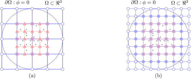
Figure 3: Sketch of the test cases with equal number of mesh points (a), and equal mesh resolution (b), respectively. Displayed are the shared (square), FFT only (triangle), and AMG only (filled circle) mesh points on a cross section of the grid plane. Illustrative particles (gray) inside the FFT domain denote the charge density.

In the following we compare accuracy and performance of the SA-AMG preconditioned conjugate gradient algorithm with a FFT-based solver. The principle difficulty in the comparison stems from the fact that the CG-based and the FFT-based solvers use different discretizations of the tube-shaped domain $\Omega$. Although both use finite-difference discretizations, with SA-AMG the whole domain is discretized while with FFT just a rectangular domain along the center line of the cylinder is taken into account. In some applications (beam pipes of light sources) the rectangular domain is contained in $\Omega$. In our application the rectangular domain has a similar volume such that the boundaries can be intertwined. Therefore, we expect that the more accurate boundary treatment in the iterative solver has a noticeable positive effect on the solution.

So, we came up with two test cases as illustrated in Figure 3.

• The first test case (a) displayed on the left corresponds to a situation where both methods have about the same number of unknowns. In the FFT-based approach only the close vicinity of the particle bunch is discretized. In contrast, in the PCG-AMG approach the grid extends to the whole domain, entailing a coarser grid than with the FFT-based approach.

• The second test case (b) displayed on the right corresponds to a situation where both methods have the same mesh resolution in the vicinity of the particles. This results in a higher number of mesh points for the PCG-AMG approach.

We consider a cylindrical tube of radius $r=0.001$ m. The FFT-based solver used a grid with $128^{2}\cdot 256=4,194,304$ nodes. The grid with a similar number of points but coarser resolution consisted of 3,236,864 grid points. To obtained the same resolution with the SAAMG-PCG solver, 5,462,016 grid points were required. They are embedded in a $166\times 166\times 256$ grid that coincides in the middle of the region of simulation with the $128\times 128\times 256$ grid for the FFT-based solver. The boundary conditions were implemented by linear extrapolation (8). In Table 7 we give execution times for the first and second iteration in a typical simulation. Since we start with quite a good vector the number of steps in the second iteration is about 30% smaller than in the first iteration. This accounts for the reduced execution time in the runs where the complete preconditioners are recomputed for each iteration. The savings from this straightforward mode to the two cases reusing either hierarchy or the entire preconditioner amounts to approximately $20\%$ and $40\%$ respectively.

solver	reusing	mesh size	mesh points	first [s]	second [s]
FFT	—	$128\times 128\times 256$	4,194,304	12.3	—
AMG	—	$128\times 128\times 256$	3,236,864	49.9	42.2
AMG	hierarchy	$128\times 128\times 256$	3,236,864	—	35.5
AMG	preconditioner	$128\times 128\times 256$	3,236,864	—	28.2
AMG	—	$166\times 166\times 256$	5,462,016	81.8	71.2
AMG	hierarchy	$166\times 166\times 256$	5,462,016	—	60.4
AMG	preconditioner	$166\times 166\times 256$	5,462,016	—	43.8

Table 7: Simulation timings of one solve in the first and second time step, respectively, with $r=0.001$ m. Equal mesh points (above) and equal mesh spacings (below) for FFT and AMG.

We inspected the SAAMG-PCG results for the two mesh sizes and found no physically relevant differences. This behaviour depends on the ratio of bunch and boundary radius. Based on the differences of the FFT and SAAMG-PCG solver (e.g. boundary treatment and implementation details) it is hard to come up with a ‘fair’ comparison. There certainly exists a correlation between the number of performed (CG) iterations and the time to solution. Determining the right stopping criteria and tolerance therefore has an important impact on the performance. While still achieving the same accuracy of the physics of a simulation it could be possible to execute fewer CG iterations by using a higher tolerance. For the measurements in Table 7 we used the stopping criterion

$$\|r\|_{2}\leq\varepsilon{\|b\|_{2}},$$

with the tolerance $\varepsilon=10^{-6}$.

These results illustrate that an increase in solution accuracy of approximately 2.3 in the best case (when the domain has irregularities) is incurred in moving from an FFT-based scheme to a more versatile approach. Of course, this more versatile approach gives rise to increased accuracy.

Coarse level solver

Another decisive portion of the AMG preconditioner is the coarse level solver. We applied either a direct solver (KLU) or used a couple of steps of Gauss-Seidel iteration. Our experiments indicate that for our problems ML setup time and scalability are not affected significantly by the two coarse level solvers. The difference in setup and application of KLU and Gauss-Seidel differ only within a few percent. Only the construction of the preconditioner is cheaper with the iterative coarse level solver.

As stated by Tuminaro & Tong [32] the number of iterations done by the iterative coarse level solver is crucial for the performance of the preconditioner. Too many iteration steps slow down the preconditioner without a corresponding increase of its quality. Too few iteration steps with the coarse level solver degrade the quality of the overall preconditioner and lead to an increased number of steps of the global system solver. We tuned the iterative coarse level solver such that the overall quality of the preconditioner was about the same as with the direct coarse level solver. It turned out that 3 iteration steps sufficed.

Coarse level size

We also tested the performance of the solver for varying sizes of the coarsest level. ML seems to perform best when the coarsest grid size is around 1000. With a limit of 1000, the coarsest grid sizes ranged from 128 to 849 when running a tube embedded in a $256\times 256\times 256$ grid on 16 to 512 cores.

At the same time we tried to set the size of the coarsest level proportional to the total available number of cores in order to get a sufficient large coarse level size. It turned out to be very difficult to set a coarse level size with heuristics like this. The factorization time increased to up to 2 s in contrast to $0.25$ s for the case where the coarsest level size is limited by 1000.

5.3 Speedup and efficiency

The efficiency of the AMG solver using linear boundary extrapolation is shown in Figure 4. On the left of this figure, the results listed in Table 8 for a $256^{3}$ grid are plotted. We observe an efficiency of approximately 62% for 256 cores relative to the timing on 16 processors, the minimal number of processors to solve the problem. The efficiency dropped just below 50% for 512 cores. The parallel efficiency is affected most by the poor scalability of the construction phase of ML. After studying various ML timings we could not identify a specific reason that causes this loss in efficiency for the construction phase other than the assumption that the problem is too small with respect to the number of cores.

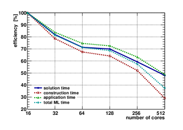
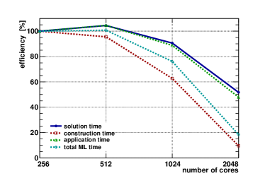
Figure 4: Efficiency for AMG on a tube embedded in a $256\times 256\times 256$ grid (left) and in a $512\times 512\times 512$ grid (right) with constant extrapolation at the boundary.

cores	solution [s]	construction [s]	application [s]	total ML [s]
16	10.91	7.75	9.52	17.28
32	6.66	4.93	5.68	10.61
64	3.82	2.87	3.19	6.06
128	1.95	1.51	1.64	3.15
256	1.15	0.93	0.94	1.88
512	0.71	0.83	0.61	1.44

Table 8: Timings for AMG on a tube embedded in a $256\times 256\times 256$ grid with linear extrapolation at the boundary.

cores	solution [s]	construction [s]	application [s]	total ML [s]
256	10.51	5.79	8.70	14.49
512	5.03	3.03	4.16	7.19
1024	2.90	2.31	2.45	4.76
2048	2.54	7.58	2.27	9.85

Table 9: Timings for AMG on a tube embedded in a $512\times 512\times 512$ grid with constant extrapolation at the boundary.

Similar conclusions can be drawn for the parallel efficiency of our solver on a $512^{3}$ grid with constant boundary treatment, see Table 9 and Figure 4. Again the construction phase of ML scales poorly for larger numbers of cores.

Notice that by applying the improvements discussed in Section 5.2, i.e., reusing (parts of) the preconditioner, the time needed for the construction phase can be reduced significantly or avoided altogether. If the preconditioner has to be built just once in an entire simulation the efficiency will get close to the 52% that we measured for the solution phase.

Finally, in Table 10 we report on timings obtained for the tube embedded in a $1024\times 1024\times 1024$ grid. In Figure 5 the corresponding efficiencies are listed. For this large problem we observe good efficiencies. The solver runs at 82% efficiency with 2048 cores relative to the 512-cores performance. The construction phase is still performing the worst with an efficiency of 73%. In this setup the problem size is still reasonably large when employing 2048 cores. This consolidates our understanding of the influence of the problem size on the low performance of the aggregation in ML.

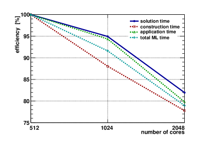
Figure 5: Efficiency for AMG on a tube embedded in a $1024\times 1024\times 1024$ grid with linear extrapolation at the boundary, corresponding to the numbers in Table 10.

cores	solution [s]	construction [s]	application [s]	total ML [s]
512	35.83	20.78	29.53	50.31
1024	18.87	11.80	15.65	27.46
2048	10.93	6.68	9.25	15.93

Table 10: Timings for AMG on a tube embedded in a $1024\times 1024\times 1024$ grid with linear extrapolation at the boundary.

Tables 8–10 provide a few data to investigate weak scability. The timings for 2048 processors in Table 10 should ideally equal those for 256 processors in Table 9. In fact, they are quite close. A comparison of the timings in Tables 9 and 8 is not so favorable. The efficiency is at most 84%. The numbers for 2048 processors in Table 9 show that the construction of the multilevel preconditioner becomes excessively expensive if the number of processors is high.

5.4 Open-space vs. PEC Boundary Conditions

In this section we compare the impact of two different boundary conditions in the setting of a physical simulation consisting of an electron source (4 MeV) followed by a beam transport section [25]. As the pipe radius gets close to the particles in the beam, the fields become nonlinear due to the image charge on the pipe. We compare the root-mean-square (rms) beam size in a field free region (drift) of a convergent beam, cf. [35, pp.171ff]. The beam pipe radius is $r=0.00085$ m in case of the PGC-MG solver. This is an extreme case in which the particles fill almost the whole beam pipe and hence the effect is very visible. The capability to have an exact representation of the fields near the boundaries is very important, because the beam pipe radius is an important optimization quantity, towards lower construction and operational costs in the design and operation of future particle accelerators.

In Figure 6 we compare rms beam sizes for the two boundary conditions applied to the boundary of a cylinder with elliptical base-area as described in Section 2.

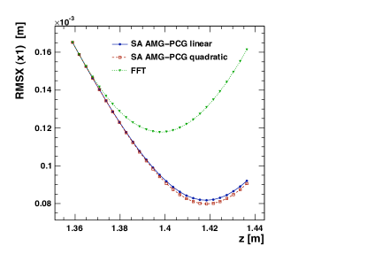
Figure 6: Comparison of rms beam size vs. position of a convergent beam. The FFT solver is applied for open-space boundary conditions, for PEC two variants of the SA AMG-PCG solver is used: with linear and quadratic boundary interpolation. (region of interest magnified). The computational domain $\Omega$ is a cylinder with $r=0.00085$ m .

The differences are up to $~{}40\%$ (at $z=1.435$ m) in rms beam size, when comparing the PEC and the open-space approach. We clearly see the shift of the beam size minimum (waste) towards larger $z$ values and a smaller minima, which means that the force of the self fields are larger when considering the beam pipe. This increase in accuracy justifies the accurate boundary treatment, in situations where the spatial extent of the beam is comparable with that of the beam pipe.

6 Conclusion

We have presented a scalable Poisson solver suitable to handle domains with irregular boundaries as they arise, for example, in beam dynamics simulations. The solver employs the conjugate gradient algorithm preconditioned by smoothed aggregation based AMG (SAAMG-PCG). PEC and open-space boundary approximations have been discussed. A real world example where the solver was used in a beam dynamics code (OPAL) shows the relevance of this approach by observing up to $~{}40\%$ difference in the RMS beam size when comparing to the FFT-based solver with open domains. The code exhibits excellent scalability up to 2048 processors with cylindrial tubes embedded in meshes with up to $1024^{3}$ grid points. In the very near future, this approach will enable precise beam dynamics simulations in large particle accelerator structures with a level of detail not obtained before.

In real particle simulations (and other test cases encountered) system matrices arising from quadratic boundary treatment are only ‘mildly’ nonsymmetric such that PCG can be applied.

Planed future work includes adaptive mesh refinement in order to reduce the number of grid points in regions that are less relevant for the space charge calculation. The boundary treatment for simply connected geometries will be extended to cope with more realistic geometries. This new method, designed for accurate 3D space charge calculations, will be used in the beam dynamics simulations for the SwissFEL project, a next generation light source foreseen to be built in Switzerland.

References

- [1] M. Adams, M. Brezina, J. Hu, R. Tuminaro, Parallel multigrid smoothing: polynomial versus Gauss–Seidel, J. Comp. Phys. 188 (2) (2003) 593–610.
- [2] A. Adelmann, C. Kraus, Y. Ineichen, J. J. Yang, The OPAL (Object Oriented Parallel Accelerator Library) Framework, Tech. Rep. PSI-PR-08-02, Paul Scherrer Institut, http://amas.web.psi.ch/docs/opal/opal_user_guide-1.1.6.pdf (2008-2010).
- [3] A. Adelmann, The IP2L (Independent Parallel Particle Layer) Framework, Tech. Rep. PSI-PR-09-05, Paul Scherrer Institut, http://amas.web.psi.ch/docs/ippl-doc/ippl_user_guide.pdf (2009-2010).
- [4] FFTPACK, a package of FORTRAN subprograms for the Fast Fourier Transform of periodic and other symmetric sequences by P. N. Swarztrauber. Available from http://www.netlib.org/fftpack/.
- [5] G. E. Forsythe, W. R. Wasow, Finite-difference methods for partial differential equations, Wiley, New York, 1960.
- [6] R. L. Gluckstern, Analytic model for halo formation in high current ion linacs, Phys. Rev. Lett. 73 (9) (1994) 1247–1250.
- [7] M. W. Gee, C. M. Siefert, J. Hu, R. S. Tuminaro, M. Sala, ML 5.0 Smoothed Aggregation User’s Guide, Tech. Report SAND2006-2649, Sandia National Laboratories (May 2006).
- [8] A. Greenbaum, Iterative Methods for Solving Linear Systems, SIAM, Philadelphia, PA, 1997.
- [9] W. Hackbusch, Multigrid Methods and Applications, Springer, Berlin, 1985.
- [10] W. Hackbusch, Iterative solution of large sparse systems of equations, Springer, Berlin, 1994.
- [11] M. A. Heroux et al., An overview of the Trilinos project, ACM Trans. Math. Softw. 31 (3) (2005) 397–423.
- [12] M. R. Hestenes, E. Stiefel, Methods of conjugent gradients for solving linear systems, J. Res. Nat. Bur. Standards 49 (1952) 409–436.
- [13] R. W. Hockney, J. W. Eastwood, Computer Simulation using Particles, Institute of Physics Publishing, Bristol, 1988.
- [14] Z. Jomaa, C. Macaskill, The embedded finite difference method for the Poisson equation in a domain with an irregular boundary and Dirichlet boundary conditions, J. Comp. Phys. 202 (2) (2005) 488 – 506.
- [15] L. D. Landau, E. M. Lifshitz, Electrodynamics of Continuous Media, 2nd Edition, Pergamon, Oxford, 1984.
- [16] R. J. LeVeque, Finite Difference Methods for Ordinary and Partial Differential Equations, SIAM, Philadelphia, PA, 2007.
- [17] P. McCorquodale, P. Colella, D. P. Grote, J.-L. Vay, A node-centered local refinement algorithm for Poisson’s equation in complex geometries, J. Comp. Phys. 201 (1) (2004) 34–60.
- [18] G. Pöplau, U. van Rienen, A self-adaptive multigrid technique for 3-D space charge calculations, IEEE Trans. Magn. 44 (6) (2008) 1242–1245.
- [19] J. Qiang, R. L. Gluckstern, Three-dimensional Poisson solver for a charged beam with large aspect ratio in a conducting pipe, Comp. Phys. Comm. 160 (2) (2004) 120–128.
- [20] J. Qiang, R. D. Ryne, Parallel 3D Poisson solver for a charged beam in a conducting pipe, Comp. Phys. Comm. 138 (1) (2001) 18–28.
- [21] F. J. Sacherer, Transverse space-charge effects in circular accelerators, Ph.D. thesis, University of California, Berkeley (1968).
- [22] F. J. Sacherer, RMS envelope equations with space charge, IEEE Trans. Nucl. Sci. 18 (3) (1971) 1105–1107.
- [23] Y. Saad, M. H. Schultz, GMRES: A generalized minimal residual algorithm for solving nonsymmetric linear systems, SIAM J. Sci. Stat. Comput. 7 (3) (1986) 856–869.
- [24] D. B. Serafini, P. McCorquodale, P. Colella, Advanced 3D Poisson solvers and particle-in-cell methods for accelerator modeling, J. Phys.: Conf. Ser. 16 (2005) 481–485.
- [25] T. Schietinger et al., Measurements and modeling at the PSI-XFEL 500-kV low-emittance electron source, in: Proceedings of the 24th Linear Accelerator Conference, Victoria, 2008, pp. 621–623, available from http://trshare.triumf.ca/~linac08proc/Proceedings/papers/tup097.pdf.
- [26] G. H. Shortley, R. Weller, The numerical solution of Laplace’s equation, J. Appl. Phys. 9 (1939) 334–344.
- [27] J. Struckmeier, M. Reiser, Theoretical studies of envelope oscillations and instabilities of mismatched intense charged-particle beams in periodic focusing channels, Part. Accel. 14 (2-3) (1984) 227–260.
- [28] P. Swarztrauber, Vectorizing the FFTs, in: G. Rodrigue (Ed.), Parallel Computations, Academic Press, New York, 1982, pp. 51–83.
- [29] The Trilinos Project Home Page, http://trilinos.sandia.gov.
- [30] U. Trottenberg, T. Clees, Multigrid software for industrial applications – from MG00 to SAMG, in: E. H. Hirschel, C. Weiland, A. Rizzi (Eds.), 100 Volumes of ‘Notes on Numerical Fluid Mechanics’, Vol. 100 of Notes on Numerical Fluid Mechanics and Multidisciplinary Design, Springer, Berlin, 2009, pp. 423–436.
- [31] U. Trottenberg, C. W. Oosterlee, A. Schüller, Multigrid, Academic Press, 2000.
- [32] R. S. Tuminaro, C. Tong, Parallel smoothed aggregation multigrid: Aggregation strategies on massively parallel machines, in: ACM/IEEE SC2000 Conference (SC2000), 2000, 21 pages, doi:10.1109/SC.2000.10008.
- [33] P. Vaněk, J. Mandel, M. Brezina, Algebraic multigrid based on smoothed aggregation for second and fourth order problems, Computing 56 (3) (1996) 179–196.
- [34] H. A. van der Vorst, Bi-CGSTAB: A fast and smoothly converging variant of Bi-CG for the solution of nonsymmetric linear systems, SIAM J. Sci. Stat. Comput. 13 (2) (1992) 631–644.
- [35] H. Wiedemann, Particle Accelerator Physics, Springer, Berlin, 2007, ”ISBN: 978-3-540-49043-2”.
- [36] D. M. Young, K. C. Jea, Generalized conjugate-gradient acceleration of nonsymmetrizable iterative methods, Linear Algebra Appl. 34 (1980) 159–194.