Stability of Binary Mixtures in Electric Field Gradients

Abstract

We consider the influence of electric field gradients on the phase behavior of nonpolar binary mixtures. Small fields give rise to smooth composition profiles, whereas large enough fields lead to a phase-separation transition. The critical field for demixing as well as the equilibrium phase separation interface are given as a function of the various system parameters. We show how the phase diagram in the temperature-composition plane is affected by electric fields, assuming a linear or nonlinear constitutive relations for the dielectric constant. Finally, we discuss the unusual case where the interface appears far from any bounding surface.

I Introduction

The effect of gravitational and magnetic fields on the phase diagram of liquid mixtures is quite small in general due to the weak coupling of the field with the mixture’s composition. The influence of electric fields was studied extensively, extensively in geometries where the field is uniform. Theoretical work predicted that for a binary mixture the upper critical solution temperature $T_{c}$ is shifted upward by a small amount, of the order of milikelvins Landau and Lifshitz (1957); Onuki (1995). Experiments in low molecular weight liquids predominantly showed an opposite shift of the same magnitude Debye and Kleboth (1965); Beaglehole (1981); Orzechowski (1999); Wirtz and Fuller (1993). Two exceptions are Reich and Gordon (1979) who measured the cloud point temperature of a polymer mixture and Gábor and Szalai (2008) who predicted a downward shift in the critical pressure of dipolar fluid mixtures in uniform electric fields.

In a uniform field the shift in $T_{c}$ is proportional to the square of electric field $E^{2}$ and $d^{2}\varepsilon/d\phi^{2}$ – the second derivative of the dielectric constant with respect to the mixture composition Onuki (2006); Schoberth et al. (2009); Tsori et al. (2006); Tsori (2009); com (a); Gunkel et al. (2007); Stepanow and Thurn-Albrecht (2009). However, in realistic systems, such as colloidal suspensions and microfluidic devices, the electric field varies in space due to the complex geometry. In such systems, electric fields on the order of $10^{7}$V/m naturally occur due to the small length-scales involved. Recently, we have shown that a homogeneous mixture confined by curved charged surfaces undergoes a phase-separation transition and two distinct domains of high and low compositions appear Tsori et al. (2004); Marcus et al. (2008). The transition occurs when the surface charge (or voltage) exceeds a critical value. In this paper we examine in detail numerically and analytically the location of the transition. We also show how this transition affects the temperature-composition phase diagram. We find that near $T_{c}$ the spatial variation of the field leads to a nontrivial modification of the stability lines. Our analysis shows that in nonuniform electric fields even a linear constitutive relation can lead to a substantial change of the transition (binodal) temperature. Lastly, we demonstrate that the phase separation interface can appear far from any of the surfaces bounding the mixture.

II Theory

Consider an A/B binary mixture confined by charged conducting surfaces giving rise to an electric field. The free energy of the mixture is

$$F=\int{\left[f_{m}(\phi,T)+f_{es}(\phi,\mathbf{E})\right]{\rm d}\mathbf{r}},$$ (1)

where $f_{m}$ is the bistable mixing free energy density, given in terms of the A-component composition $\phi$ ($0<\phi<1$) and the temperature $T$.

$f_{es}$ is the electrostatic free energy density due to the electric field $\mathbf{E}$, given by

$$f_{es}=-\frac{1}{2}\varepsilon(\phi)(\nabla\psi)^{2}.$$ (2)

$\psi$ is the electrostatic potential. The negative sign corresponds to cases where the potential is prescribed on the bounding surfaces. When the charge is given on the bounding surfaces the sign should be replaced by a positive one Landau et al. (1984); Onuki (2004a, 2006). $\varepsilon$ is the mixture’s permittivity, and is a function of the composition $\phi$. Note that in order to isolate the electric field effect we do not include any direct short- or long-range interactions between the liquid and the confining surfaces. The equilibrium composition profile $\phi(\mathbf{r})$ and electrostatic potential $\psi(\mathbf{r})$ are given by the extremization of the free energy with respect to $\phi$ and $\psi$ Onuki and Kitamura (2004); Onuki (2004b). The resulting Euler-Lagrange equations are

$$\frac{\delta F}{\delta\phi} = \frac{\delta f_{m}}{\delta\phi}-\frac{1}{2}\frac{d\varepsilon(\phi)}{d\phi}(\nabla\psi)^{2}-\mu=0,$$ (3)

$$\frac{\delta F}{\delta\psi} = \nabla\cdot(\varepsilon(\phi)\nabla\psi)=0.$$ (4)

Eq. (4) is simply Gauss’s law. Notice that the relation $\varepsilon(\phi)$ couples these nonlinear equations. In the canonical ensemble $\mu$ is a Lagrange multiplier adjusted to satisfy mass conservation:

$$\int{\left[\phi(\mathbf{r})-\phi_{0}\right]{\rm d}\mathbf{r}}=0,$$ (5)

where $\phi_{0}$ is the average composition. In the case of a system in contact with a matter reservoir (grand-canonical ensemble), the chemical potential is set by the reservoir, $\mu=\mu(\phi_{0})$ where $\phi_{0}$ is the reservoir composition.

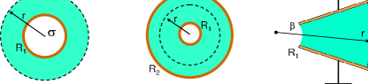
Figure 1: The three model systems. (a) A single charged spherical colloid with surface charge density $\sigma$ and radius $R_{1}$. (b) A charged wire with surface charge density $\sigma$ and radius $R_{1}$, or two concentric cylinders with radii $R_{1}$ and $R_{2}$. (c) A wedge comprised of two flat electrodes with an opening angle $\beta$ and potential difference $V$. $R_{1}$ and $R_{2}$ are the minimal and maximal values of the distance $r$ from the imaginary meeting point of the electrodes.

In order to simplify the solution of Eqs. (3)–(5), we consider the three simple model systems shown schematically in Fig. 1. The first one is a charged isolated spherical colloid of radius $R_{1}$ and surface charge density $\sigma$, immersed in an infinite mixture bath. In this system, spherical symmetry dictates that $\phi=\phi(r)$ and $\mathbf{E}=\mathbf{E}(r)$ where r is the distance from the colloid’s center. Since the colloid has a prescribed charge we can integrate Gauss’s law and obtain an explicit expression for the electric field: $\mathbf{E}(r)=\sigma R_{1}^{2}/(\varepsilon(\phi)r^{2})\hat{\mathbf{r}}$. The second geometry is a charged wire of radius $R_{1}$ and surface charge density $\sigma$, coupled to a reservoir at $r\rightarrow\infty$. Alternatively, we may consider a closed condenser made up of two concentric cylinders of radii $R_{1}$ and $R_{2}$. In both cases, we readily obtain the electric field $\mathbf{E}(r)=\sigma R_{1}/(\varepsilon(\phi)r)\hat{\mathbf{r}}$, where $r$ is the distance from the inner cylinder’s center. The last system is the wedge condenser, made up from two flat electrodes with an opening angle $\beta$ and a potential difference $V$ across them. Solution of the Laplace equation gives $\mathbf{E}(r)=(V/\beta r)\hat{\mathbf{\theta}}$, where $r$ is the distance from the imaginary meeting point of the electrodes and $\theta$ is the azimuthal angle. In this geometry $\phi=\phi(r)$ and therefore $\mathbf{E}\cdot\nabla\varepsilon=0$. The explicit expressions for the electric field in all three systems outlined above decouple equations (3) and (4).

We will show that Eq. (3) leads, under certain conditions, to a phase-separation transition. This transition is independent of the exact form of $f_{m}$, and can be realized as long as $f_{m}$ is bistable and the dielectric constant $\varepsilon$ depends on the composition $\phi$. In order to be specific, we will consider the mixing free energy derived from the Flory-Huggins lattice theory, with lattice site volume $v_{0}$. We consider the simple symmetric case where each component occupies $N$ successive lattice cells. Simple liquids have $N=1$, while polymers have $N>1$ monomers. The mixing free energy density is then given by $f_{m}=k_{B}T\tilde{f}_{m}/Nv_{0}$, where

$$\tilde{f}_{m}=\phi\log(\phi)+(1-\phi)\log(1-\phi)+N\chi\phi(1-\phi).$$ (6)

$k_{B}$ is the Boltzmann constant, and $\chi\sim 1/T$ is the Flory interaction parameter Doi (1996). We limit ourselves to the case where $\chi>0$, leading to an Upper Critical Solution Temperature type phase diagram in the $\phi-T$ plane. In the absence of electric field, the mixture is homogeneous above the binodal curve $\phi_{t}(T)$, and phase separates into two phases having the binodal compositions $\phi_{t}$ below it. Below the binodal curve, but above the spinodal, given by $\phi_{s}(T)=(1/2)[1\pm\sqrt{1-2/(N\chi)}]$, the mixture is metastable. The binodal and spinodal curves meet at the critical point $(\phi_{c},(N\chi)_{c})=(1/2,2)$. The transition (binodal) temperature $T_{t}$ for a given composition is given by $T_{t}(\phi)=(N\chi)_{c}T_{c}\left[\log(\phi/(1-\phi))/(2\phi-1)\right]^{-1}$ Doi (1996).

Using the expressions given above for the electric field, we write the generalized composition equation valid for cylindrical and spherical geometries:

$$\tilde{f}^{\prime}_{m}(\phi)-N\chi M_{{\rm sc}}\frac{d\tilde{\varepsilon}/d\phi}{\tilde{\varepsilon}^{2}(\phi)}\tilde{r}^{-n}-\tilde{\mu}=0.$$ (7)

Here, $\tilde{r}\equiv r/R_{1}$ is the scaled distance and $\tilde{\varepsilon}=\varepsilon/\varepsilon_{0}$, with $\varepsilon_{0}$ the vacuum permittivity. Where

$$M_{{\rm sc}}\equiv\frac{\sigma^{2}Nv_{0}}{4k_{B}T_{c}\varepsilon_{0}}$$ (8)

is the dimensionless field, and $n$ is an exponent characterizing the decay of $E^{2}$: $n=2$ for concentric cylinders, and $n=4$ for spherical colloid. For the wedge geometry we find:

$$\tilde{f}^{\prime}_{m}(\phi)-N\chi M_{{\rm w}}\frac{d\tilde{\varepsilon}}{d\phi}\tilde{r}^{-n}-\tilde{\mu}=0,$$ (9)

where

$$M_{{\rm w}}\equiv\frac{V^{2}Nv_{0}\varepsilon_{0}}{4\beta^{2}k_{B}T_{c}R_{1}^{2}},$$ (10)

and $n=2$. $M_{{\rm sc}}$ and $M_{{\rm w}}$ are dimensionless quantities measuring the magnitude of the maximal electrostatic energy stored in a molecular volume compared to the thermal energy. The second term in Eqs. (7) and (9) is the variation of the electrostatic free energy with respect to $\phi$, and is only present when the mixture components have different permittivities.

The constitutive relation $\tilde{\varepsilon}(\phi)$ is a smooth function of $\phi$. Experiments show that the curve can be slightly convex or concave, and is dominantly linear Debye and Kleboth (1965); Beaglehole (1981); Akhadov (1981). They are mostly in agreement with Clausius-Mossotti and Onsager-based theories for the dielectric constant Sen et al. (1992). Thus, for a mixture of liquids A and B with dielectric constants $\tilde{\varepsilon}_{a}$ and $\tilde{\varepsilon}_{b}$, respectively, the experiments yield a polynomial relation in the form

$$\tilde{\varepsilon}(\phi)\simeq\tilde{\varepsilon}_{b}+\tilde{\varepsilon}^{\prime}\phi+\tilde{\varepsilon}^{\prime\prime}\phi^{2}+.~{}.~{}.~{}.$$ (11)

We start by focusing on a linear relation, namely $\tilde{\varepsilon}^{\prime\prime}=0$; in this case $\tilde{\varepsilon}^{\prime}=\Delta\tilde{\varepsilon}\equiv\tilde{\varepsilon}_{a}-\tilde{\varepsilon}_{b}$. Even in such a simple case it turns out that a phase separation transition occurs, in contrast to the Landau mechanism which relies on a nonvanishing $\tilde{\varepsilon}^{\prime\prime}$. After investigating linear relations we examine how our results change when $\tilde{\varepsilon}(\phi)$ has a positive or negative curvature, by allowing for $\tilde{\varepsilon}^{\prime\prime}\neq 0$. In this case $\tilde{\varepsilon}^{\prime}$ is different from $\Delta\tilde{\varepsilon}$. Higher order terms in the expansion Eq. (11) are not expected to change the results qualitatively, since they do not affect much the curvature of $\tilde{\varepsilon}(\phi)$Debye and Kleboth (1965); Beaglehole (1981); Akhadov (1981).

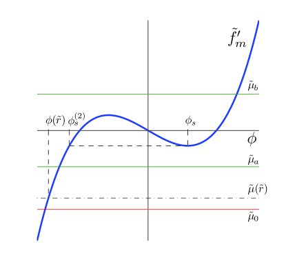
Figure 2: Graphical solution of Eq. (12) for an open wedge at $T<T_{c}$ and a symmetric mixture. Solid curve is $\tilde{f}^{\prime}_{m}(\phi)$. Its roots are the transition (binodal) compositions. The intersection between $\tilde{f}^{\prime}_{m}(\phi)$ and the horizontal dash-dotted line $\tilde{\mu}(\tilde{r})$ gives the composition $\phi(\tilde{r})$. If $\tilde{\mu}(\tilde{R}_{1})$ is at $\tilde{\mu}_{a}$, the profile $\phi(\tilde{r})$ varies smoothly, but if $\tilde{\mu}(\tilde{R}_{1})=\tilde{\mu}_{b}$, $\phi(\tilde{r})$ has a discontinuity.

III Results and Discussion

Before we present the numerical solutions of Eqs. (7) and (9), it is illustrative to consider a graphical solution for a wedge condenser. Recall that in the absence of field it is assumed that $T$ is above the binodal temperature. We rewrite Eq. (9) as:

$$\begin{split}\tilde{f}^{\prime}_{m}(\phi)&=\tilde{\mu}(\tilde{r})\\ \tilde{\mu}(\tilde{r})&\equiv\frac{N\chi\Delta\tilde{\varepsilon}M_{{\rm w}}}{\tilde{r}^{2}}+\tilde{\mu}_{0}\end{split}$$ (12)

where $\tilde{\mu}_{0}$ is the dimensionless reservoir chemical potential. At a given temperature, the intersection of $\tilde{f}^{\prime}_{m}(\phi)$ and the horizontal line $\tilde{\mu}(\tilde{r})$ gives the local composition $\phi(\tilde{r})$ (Fig. 2). When $\tilde{r}\rightarrow\infty$, $\tilde{\mu}(\tilde{r})\rightarrow\tilde{\mu}_{0}$ and the composition is $\phi=\phi_{0}$, corresponding to a homogeneous phase. For simplicity we consider $\phi_{0}<\phi_{c}$. As $\tilde{r}$ decreases, $\tilde{\mu}(\tilde{r})$ (and hence $\phi(\tilde{r})$) increase until they attain their maximal value at $\tilde{R}_{1}$. Above $T_{c}$, the free energy is always convex, $\tilde{f}^{\prime}_{m}$ is a monotonic function of $\phi$, and the composition profile $\phi(\tilde{r})$ is hence continuous. However, below $T_{c}$, $\tilde{f}_{m}$ is bistable and $\tilde{f}^{\prime}_{m}$ is sigmoidal. In this case there are two possible scenarios shown in Fig. 2. If, for example, $\tilde{\mu}(\tilde{R}_{1})=\tilde{\mu}_{a}$, the composition profile varies smoothly. If, on the other hand, $\tilde{\mu}(\tilde{R}_{1})=\tilde{\mu}_{b}$, there is a discontinuity in the profile since there is a radius $\tilde{R}>\tilde{R}_{1}$ where the value of $\phi$ can “jump” from high to low values. Below $T_{c}$, there is a range of radii, or compositions, where the discontinuity in $\phi(\tilde{r})$ can occur. The equilibrium profile $\phi(\tilde{r};\tilde{R})$ is the one that minimizes the total free energy integral $F=\int f[\phi(\tilde{r};\tilde{R})]{\rm d}r$. These conclusions also hold for Eq. (7).

In Fig. 2 we show the composition $\phi_{s}^{(2)}$ defined by the relation $\tilde{f}^{\prime}_{m}(\phi_{s}^{(2)})=\tilde{f}^{\prime}_{m}(\phi_{s})$. Clearly, this is the minimal composition for which exist more than one solution to Eq. (9). The role of this special composition will be discussed later.

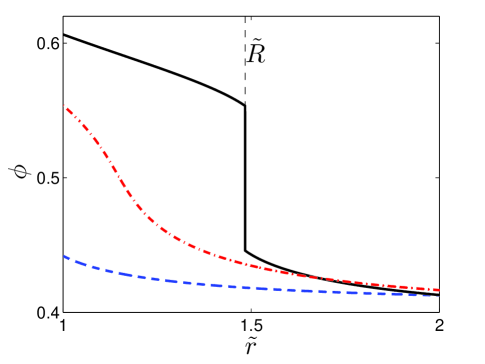
Figure 3: The three types of equilibrium profiles $\phi(\tilde{r})$ for a system of two concentric cylinders. Dash-dot line: $T=1.005T_{c}$ and $M_{{\rm sc}}=0.04$: above $T_{c}$ the profile is smoothly varying. Dashed line: $T=0.995T_{c}$, $M_{{\rm sc}}=0.01$ smaller than the critical value for demixing. Solid line: same $T$, but $M_{{\rm sc}}=0.04$ is large enough to induce phase separation marked by an interface at $\tilde{r}=\tilde{R}$. We took an average composition $\phi_{0}=0.41$. Here and in other figures, $\tilde{R}_{1}=1$, $\tilde{R}_{2}=5$, $\tilde{\varepsilon}_{a}=5$, and $\tilde{\varepsilon}_{b}=3$.

The three typical composition profiles are shown in Fig. 3. Above $T_{c}$ (dash-dot line), $\phi(\tilde{r})$ varies smoothly due to the dielectrophoretic force, whereby the high-$\tilde{\varepsilon}$ liquid is drawn into the strong electric field region. Below $T_{c}$ (dashed line), at a temperature where the field-free mixture is homogeneous, if $M$ is small the profile $\phi(\tilde{r})$ is again smoothly decaying, exhibiting the same dielectrophoretic behavior. However, if at the same temperature, $M$ is increased, either by adding charge to the surface or by increasing the curvature (smaller $R_{1}$), we arrive at a critical value, denoted $M^{*}$. Above it, a phase-separation transition occurs. This is shown in the solid line of Fig. 3, where the mixture consists of two coexisting domains separated by an interface at $\tilde{r}=\tilde{R}$.

The typical value of charge/voltage required for demixing can be estimated from the value of $M$ being in the range $M\sim 0.001-0.1$ Marcus et al. (2008). Consider a colloid of radius $R_{1}\sim 1\mu$m placed in a mixture having a molecular volume $Nv_{0}\simeq 5\times 10^{-27}$m³ and $T_{c}\simeq 300$K. Then, the typical demixing charge is of the order of $10^{2}-10^{4}e$ charges (surface voltage is $1-100V$). It scales linearly with $1/N$: in a polymer mixture the confining surfaces require $N$ times smaller charge compared to molecular liquids in order to induce phase separation.

III.1 The phase-separation interface

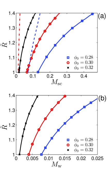
Figure 4: Location of the demixing interface $\tilde{R}$ as a function of $M$, (a) for three average compositions $\phi_{0}$ in a closed cylindrical system (lines with symbols) and for $\phi_{0}=0.28$ (dashed line) and $\phi_{0}=0.3$ (dash-dot line) in an open system. Curves do not coincide at $\tilde{R}=1$. (b) The same, in the closed ”wedge” geometry. We took $T=0.96T_{c}$.

At the critical value of $M$, a sharp interface first appears separating coexisting regions of high- and low-$\phi$ value. If the average composition $\phi_{0}$ is smaller than $\phi_{c}$, the interface appears at $\tilde{r}=\tilde{R}_{1}$. When we further increase $M$ and supply more electrostatic energy to the system, dielectrophoresis leads to an increase in the size of the high composition domain. Thus, the location of the separation interface $\tilde{R}$ increases. Fig. 4 shows how $\tilde{R}$ varies with $M$ at a constant temperature in the concentric cylinders and wedge systems. Notice that as $\phi_{0}$ approaches the binodal composition ($\phi_{t}\simeq 0.33$), $\tilde{R}$ is larger at the same $M$. It also grows more rapidly with increasing $\phi_{0}$. Indeed, when the binodal is approached, the mixing free energy barrier is smaller. Secondly, $\tilde{R}$ grows faster in an open system than in a closed one. This is because in a closed system the energy penalty in $\tilde{f}_{m}$ grows faster than the energy gain in $\tilde{f}_{es}$. Material conservation gives the maximum value of $\tilde{R}$, $\tilde{R}_{\infty}$, given by

$$\tilde{R}^{2}_{\infty}=\phi_{0}(\tilde{R}_{2}^{2}-\tilde{R}_{1}^{2})+\tilde{R}_{1}^{2}.$$ (13)

This $M\rightarrow\infty$ limit is physically unattainable and is preempted by dielectric breakdown.

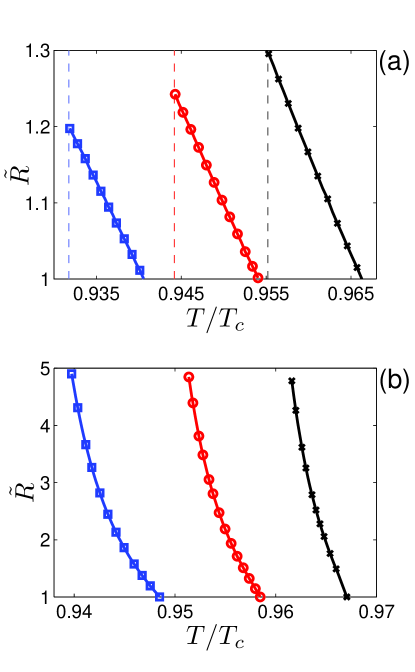
Figure 5: Location of the demixing interface $\tilde{R}$ as a function of $T/T_{c}$, (a) for three average compositions in a closed cylindrical system: $\phi_{0}=0.28$ (squares), $0.3$ (circles) and $0.32$ (crosses) with $M_{{\rm sc}}=0.04$. When $\tilde{R}=\tilde{R}_{1}$, the temperature corresponds to $M_{{\rm sc}}=M_{{\rm sc}}^{*}=0.04$. $\tilde{R}$ grows as $T/T_{c}$ is reduced until it attains it maximal value at the binodal temperature (dashed line for each value of $\phi_{0}$) (b) Same, in an open cylindrical system with $M_{{\rm sc}}=0.004$. Here, $\tilde{R}\rightarrow\infty$ at the binodal.

Note that the typical values of $M$ in the cylindrical and spherical cases are an order of magnitude larger than in the wedge condenser, see Fig. 4 (a) and (b). Indeed, in the spherical and cylindrical symmetries, $\mathbf{E}$ is parallel to $\nabla\phi$: the dielectrophoretic force, (proportional $\Delta\varepsilon$), has to be large enough to overcome the energy penalty associated with dielectric interfaces parallel to $\mathbf{E}$ (proportional to $(\Delta\varepsilon)^{2}$) Tsori (2009). On the other hand, in the wedge condenser $\mathbf{E}$ is perpendicular to $\nabla\phi$, and the required dielectrophoretic force for demixing is correspondingly smaller, leading to smaller values of $M_{{\rm w}}$. This could be seen by comparing the electrostatic terms in Eqs. (3) and (4), differing by a factor of $\tilde{\varepsilon}(\phi)^{-2}\sim 0.1$, which $M_{{\rm sc}}$ has to compensate for in order for the values of $\tilde{f}_{es}$ to be equal.

Alternatively, an increase in $T$ at constant electric field decreases $\chi M\sim M/T$ and decreases $\tilde{R}$. Fig. 5 shows how an increase in $T$ shrinks the high-$\phi$ domain and decreases $\tilde{R}$ in a closed and open cylindrical system. In Fig. 5, when $\tilde{R}=1$ the temperature is that for which $M=M^{*}$. The effect of temperature is much more pronounced in an open system: $\tilde{R}$ tends to infinity when approaching the binodal temperature (not shown). On the other hand, $\tilde{R}$ is finite when approaching the binodal in a closed system. Its maximal value is larger when $|\phi_{0}-\phi_{c}|$ is smaller, because then the mixing free energy difference between low- and high-$\phi$ values is reduced. In Fig. 5 (a), $\tilde{R}$ appears to be linear simply because $T$ changes over a small interval.

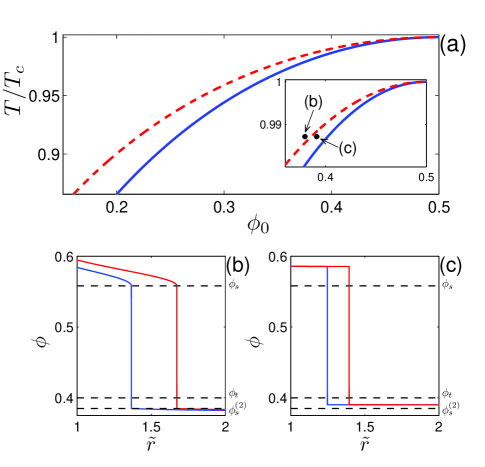
Figure 6: (a) The “differentiating” curve – $\phi^{\dagger}$ (dashed line) for an open wedge. Above it, when phase separation occurs, the composition at the interface jumps from $\phi_{s}^{(2)}$ to $\phi_{s}$. Below $\phi^{\dagger}$ the front composition jumps from $\phi_{s}^{(2)}<\phi_{1}<\phi_{t}$ to $\phi_{2}>\phi_{s}$. Examples of this behavior are shown in (b) and (c), where composition profiles for points above and below $\phi^{\dagger}$ with two values of $M$ are given, showing this behavior is independent of $M$. The inset in (a) is a blowup showing the location of (b) and (c) in the $\phi_{0}-T$ plane. In (b) $\phi_{0}=0.38$ with $M_{{\rm w}}=4\times 10^{-4}$ and $M_{{\rm w}}=6\times 10^{-4}$, and in (c) $\phi_{0}=0.39$ with $M_{{\rm w}}=1\times 10^{-5}$ and $M_{{\rm w}}=1.5\times 10^{-5}$. In (b) and (c) we took $T=0.987T_{c}$.

One can estimate the value of $\phi$ at the demixing interface in an open system. At the interface there is a “jump” in $\phi(\tilde{r})$ from $\phi_{1}$ to $\phi_{2}>\phi_{1}$. Let us denote by $\phi(\tilde{R})$ the upper interface composition – $\phi(\tilde{R})=\phi_{2}$. The conditions for a “jump” in the wedge geometry are:

$$\tilde{f}_{m}^{\prime}(\phi_{1})-N\chi\frac{\Delta\tilde{\varepsilon}M_{{\rm w}}}{\tilde{R}^{2}}-\tilde{\mu}_{0}=0,$$ (14)

$$\tilde{f}_{m}^{\prime}(\phi_{2})-N\chi\frac{\Delta\tilde{\varepsilon}M_{{\rm w}}}{\tilde{R}^{2}}-\tilde{\mu}_{0}=0,$$ (15)

$$\tilde{f}_{m}(\phi_{1})-N\chi\frac{\tilde{\varepsilon}(\phi_{1})M_{{\rm w}}}{\tilde{R}^{2}}\geq\tilde{f}_{m}(\phi_{2})-N\chi\frac{\tilde{\varepsilon}(\phi_{2})M_{{\rm w}}}{\tilde{R}^{2}}.$$ (16)

The first two equations define the local solutions of Eq. (12), and the third one is the condition that a high composition is favorable: $\tilde{f}(\phi_{2})<\tilde{f}(\phi_{1})$. The true value of $\tilde{R}$ is the one that gives the global minimum of the free energy. Putting Eq. (14) in Eq. (16) and using $\tilde{\mu}_{0}=\tilde{f}_{m}^{\prime}(\phi_{0})$, we get

$$\tilde{f}_{m}^{\prime}(\phi_{1})-\tilde{f}_{m}^{\prime}(\phi_{0})\geq\frac{\tilde{f}_{m}(\phi_{2})-\tilde{f}_{m}(\phi_{1})}{\phi_{2}-\phi_{1}}.$$ (17)

The right-hand side of Eq. (17) is maximal when the transition occurs from $\phi_{1}=\phi_{s}^{(2)}$ to $\phi_{2}=\phi_{s}$ ($\phi_{s}^{(2)}<\phi_{s}$). We therefore denote $\Delta f_{{\rm w,max}}$ by

$$\Delta f_{{\rm w,max}}=\frac{\tilde{f}_{m}(\phi_{s})-\tilde{f}_{m}(\phi_{s}^{(2)})}{\phi_{s}-\phi_{s}^{(2)}}.$$ (18)

If the inequality

$$\tilde{f}_{m}^{\prime}(\phi_{1})-\tilde{f}_{m}^{\prime}(\phi_{0})\geq\Delta f_{{\rm w,max}}$$ (19)

holds, the transition must be at $\phi_{1}=\phi_{s}^{(2)}$, since for larger values of $\phi_{1}$ the right-hand side of Eq. (17) is smaller while the left-hand side is larger, so a higher composition is surely favored. The equality sign in Eq. (19) corresponds to the maximal average composition $\phi_{0}$ for which this equation holds.

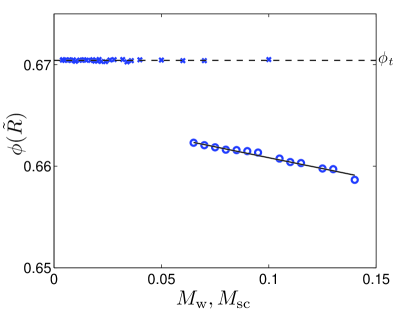
Figure 7: Composition at the demixing interface $\tilde{R}$ as a function of $M$ for a closed wedge (crosses) and concentric cylinders (circles). The dashed line is the binodal composition. Here $\phi_{0}=0.3$ and $T=0.96T_{c}$.

The locus of such compositions is the “differentiating curve” – $\phi^{\dagger}$, shown in the dashed curve of Fig. 6 (a). When the zero-field point in the phase diagram $(\phi_{0},T)$ is above the $\phi^{\dagger}(T)$ curve, Eq. (19) holds, and the composition at the interface jumps from $\phi_{s}^{(2)}$ to $\phi_{s}$ com (b). When $(\phi_{0},T)$ is below $\phi^{\dagger}(T)$ the upper interface composition $\phi(\tilde{R})$ is between $\phi_{s}$ and $\phi_{t}$. Eq. (17) shows this result is independent of $M$. An example of this situation is given in Fig. 6 (b), where the compositions $\phi_{1}$ and $\phi_{2}$ are the same for two values of $M$. Fig. 6 (c) shows the interface compositions are independent of $M$ also when $\phi_{0}$ is larger than $\phi^{\dagger}$.

When the discontinuity in the composition profile occurs at $\phi_{2}=\phi_{s}$, we can invert Eq. (9) to get $\tilde{R}\propto M^{1/2}$ for the open wedge system. In particular, above the differentiating curve we get in the Flory-Huggins model

$$\tilde{R}=\left[\frac{N\chi\Delta\tilde{\varepsilon}M_{{\rm w}}}{\tilde{f}_{m}^{\prime}(\phi_{s})-\tilde{\mu}_{0}}\right]^{1/2}.$$ (20)

Thus, $\tilde{R}$ varies linearly with the wedge potential $V$.

In the other geometries $\tilde{f}^{\prime}_{es}$ depends on $\phi$, and this influences the value of pairs $\phi_{1}$ and $\phi_{2}$. However, a very good approximation, valid when $M_{{\rm sc}}$ is not too large and $T$ is not too close to $T_{c}$, is that the transition remains from $\phi_{1}=\phi_{s}^{(2)}$ to $\phi_{2}=\phi_{s}$. One can then repeat a similar derivation and obtain

$$\tilde{f}_{m}^{\prime}(\phi_{1})-\tilde{f}_{m}^{\prime}(\phi_{0})\geq\Delta f_{{\rm sc,max}},$$ (21)

$$\Delta f_{{\rm sc,max}}=\frac{\tilde{f}_{m}(\phi_{s})-\tilde{f}_{m}(\phi_{s}^{(2)})}{\phi_{s}-\phi_{s}^{(2)}}\frac{\tilde{\varepsilon}(\phi_{s})}{\tilde{\varepsilon}(\phi_{s}^{(2)})}.$$ (22)

Using these equations one can determine the differentiating curve for cylindrical and spherical geometries.

The situation is different in a closed system, as Fig. 7 shows. In the wedge, the demixing interface occurs at the binodal composition, $\phi_{t}$, irrespective of $M$. In the cylindrical and spherical systems, $\phi(\tilde{R})$ is lower than but close to $\phi_{t}$, and decreases when $M$ grows. The qualitative explanation is as follows. In the wedge geometry $\tilde{f}^{\prime}_{es}$ only adds a constant to $\tilde{f}^{\prime}$, and the binodal compositions remain the only pair of solutions of Eq. (9) that have the same mixing free energy $\tilde{f}_{m}$. Hence, the mixing free energy penalty is minimized when the transition is at the binodal compositions Landau and Lifshitz (1980). This also explains why in the wedge geometry $\phi(\tilde{R})$ is independent of $M$. In the cylindrical and spherical geometries on the other hand, $\tilde{f}^{\prime}_{es}$ affects $\phi(\tilde{R})$, resulting in a value of $\phi(\tilde{R})$ smaller than $\phi_{t}$. This reflects the fact that dielectrophoresis favors high values of $\phi$. Since $\tilde{f}_{es}\propto M$, larger values of $M$ lead to lower values of $\phi(\tilde{R})$.

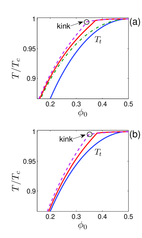
Figure 8: (a) Stability diagram of a spherical colloid with $M_{{\rm sc}}=0.04$ (thick solid line) and $M_{{\rm sc}}=0.08$ (dashed line). Dash-dot curve is $\phi^{\dagger}$ [see Fig. 6(a)] and thin solid line is the binodal $T_{t}(\phi_{0})$ . (b) Stability diagram showing $\phi^{*}(T)$ for concentric cylinders with $M_{{\rm sc}}=0.04$ (thick solid line) and $M_{{\rm sc}}=0.08$ (dashed line).

III.2 Stability diagrams

One can also set $M$ constant and for a given electric field draw the a stability curve $\phi^{*}(T)$ in the $\phi_{0}-T$ plane, see Fig. 8. $\phi^{*}(T)$ is defined such that below it phase separation occurs, while above it composition profiles are smooth. Fig. 8 (a) and (b) show the stability diagram of a spherical colloid and concentric cylinders, respectively. In both diagrams, an increase in $M$ increases the unstable region. For the same value of $M$, in a closed system the phase separation region is smaller than in an open one, because the mixing energy penalty makes it more difficult to induce phase separation. The range of values of $\phi_{0}$ that are unstable in nonuniform electric fields grows when $T$ increases (but still $T<T_{c}$). For low values of $T$, there is a significant difference between open and closed systems: in open systems, if $M$ is large enough the stability curve tends to $\phi^{\dagger}$ [see Fig. 6(a)], whereas for closed systems the stability curve tends to $\phi_{t}$ where demixing is spontaneous.

In both parts of Fig. 8, there is a kink in all the curves $\phi^{*}(T)$ at a temperature we denote $T_{k,1}$. In the Flory-Huggins model and for spherical colloids and concentric cylinders, the second derivative of the free energy is

$$\frac{\partial^{2}\tilde{f}}{\partial\phi^{2}}=\frac{\partial^{2}\tilde{f}_{m}}{\partial\phi^{2}}+2N\chi M_{{\rm sc}}\frac{(d\tilde{\varepsilon}/d\phi)^{2}}{\tilde{\varepsilon}^{3}(\phi)}\tilde{r}^{-n}.$$ (23)

The second term in this equation is the positive electrostatic contribution $f^{\prime\prime}_{es}$. It is clear that when an electric field is present, even at $T<T_{c}$, the electrostatic contribution can lead to a positive value of $\tilde{f}^{\prime\prime}(\phi,\tilde{r})$ and phase separation cannot occur.

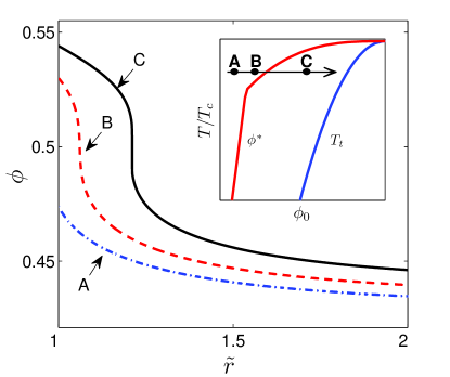
Figure 9: Composition profiles above the kink temperature for an isolated spherical colloid. The profiles change from smooth (dash-dot and dashed lines) to discontinuous (solid line) with a discontinuity at finite value of $\tilde{R}$: $\tilde{R}_{1}\leq\tilde{R}\leq\tilde{R}_{2}$, when $\phi_{0}$ increases at constant $T$ and $M$ (see inset).

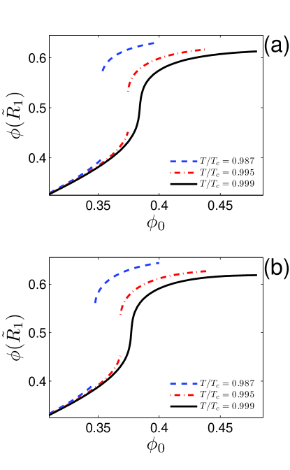
Figure 10: Surface composition $\phi(\tilde{R}_{1})$ when approaching the binodal, (a) for three temperatures in a closed cylindrical system. (b) Same, for an isolated charged cylinder. We took $M_{{\rm sc}}=0.04$.

When $T<T_{k,1}$, $\tilde{f}^{\prime\prime}$ is negative for all values of $\tilde{r}$, and the phase separation interface appears first at $\tilde{R}=\tilde{R}_{1}$. However, when $T>T_{k,1}$, for a given value of $\phi_{0}$, a special radius $\tilde{R}_{c}(T,\phi_{0})$ exists. This is the largest value of $\tilde{r}$ for which $\tilde{f}^{\prime\prime}$ in Eq. (23) can be negative. In this case, the demixing interface appears first at $\tilde{R}=\tilde{R}_{c}$. An example of this behavior is shown in Fig. 9: at constant $T_{c}>T>T_{k,1}$, at points A and B ($\phi_{0}<\phi^{*}$) $\phi(\tilde{r})$ is smooth, similar to $\phi(r)$ above $T_{c}$. However, at point C ($\phi_{0}>\phi^{*}$) $\phi(r)$ has a discontinuity at $\tilde{R}>\tilde{R}_{c}$. As the critical point is approached, $\tilde{R}_{c}\rightarrow\infty$ and $\phi^{*}$ approaches the critical composition.

The kink temperature $T_{k,1}$ is given by setting $\tilde{R}_{c}=\tilde{R}_{1}$ and can be obtained from solution of:

$$\frac{\partial^{2}\tilde{f}}{\partial\phi^{2}}(\tilde{R}_{1})=0,\ \frac{\partial^{3}\tilde{f}}{\partial\phi^{3}}(\tilde{R}_{1})=0.$$ (24)

We stress that this result is independent of the exact form of mixing free energy. Notice that for a wedge, the electric field has no effect on the convexity of the free energy, and one finds $T_{k,1}=T_{c}$ (see Fig. 11).

The surface composition $\phi(\tilde{R}_{1})$ when approaching the binodal at constant $T$ and $M$ is given in Fig. 10. When $T<T_{k,1}$ the surface composition has a discontinuity at $\phi_{0}=\phi^{*}$ (dashed and dash-dot lines) and the value of $\phi(\tilde{R}_{1})$ becomes larger than $\phi_{c}$. When $T>T_{k,1}$ the surface composition varies smoothly (solid lines). The discontinuity in $\phi(\tilde{R}_{1})$ occurs at lower values of $\phi_{0}$ in open systems compared to closed ones; open systems are less stable than closed systems. When $T$ increases at a given value of $\phi_{0}$, the surface composition decreases since mixing is favored at high temperatures.

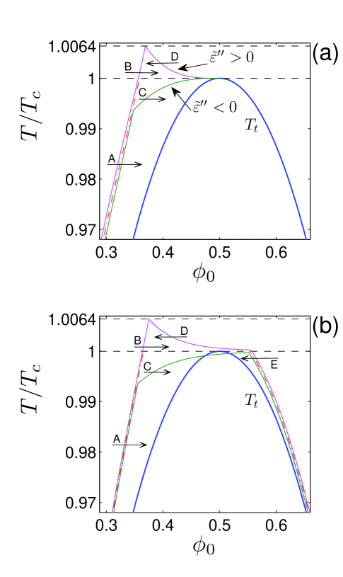
Figure 11: (a) Stability diagram for an open wedge with $M_{{\rm w}}=4\times 10^{-3}$ and three constitutive relations Eq. (11) with $\tilde{\varepsilon}_{a}=5$ and $\tilde{\varepsilon}_{b}=3$. Thick solid line is the transition (binodal) curve $T_{t}(\phi)$. When $\tilde{\varepsilon}^{\prime\prime}=0$ (dash-dot line) there is no phase separation above $T_{c}$. For $\tilde{\varepsilon}^{\prime\prime}=1.6$ an unstable region exists above $T_{c}$. In contrast, when $\tilde{\varepsilon}^{\prime\prime}=-1.6$ is negative, the unstable region is suppressed. $\phi(\tilde{r})$ changes from smooth to discontinuous at $\tilde{R}_{1}$ along lines A and B, and at $\tilde{R}_{c}>\tilde{R}_{1}$ along C and D. (b) The same for a closed wedge system. Note that the stability curve extends to compositions larger than $\phi_{c}$. $\phi(\tilde{r})$ changes from smooth to discontinuous at $\tilde{R}_{1}$ along A and B, at $\tilde{R}_{1}<\tilde{R}_{c}<\tilde{R}_{2}$ along C and D, and at $\tilde{R}_{2}$ along E. Here $T_{k,1}/T_{c}=1.0064$.

III.3 Quadratic constitutive relation

We now examine how the stability diagram changes if the dielectric constant has a quadratic dependence on composition: $\tilde{\varepsilon}^{\prime\prime}\neq 0$ in Eq. (11). For simplicity, we treat the wedge system where a linear constitutive relation means that $T_{k,1}=T_{c}$. In the Flory-Huggins model, the conditions in Eq. (24) give

$$\frac{T_{k,1}}{T_{c}}=1+M_{{\rm w}}\tilde{\varepsilon}^{\prime\prime},$$ (25)

where we used $\tilde{R}_{1}=1$.

Note that $\tilde{\varepsilon}^{\prime\prime}$ can be positive or negative. When $\tilde{\varepsilon}^{\prime\prime}<0$, $\tilde{f}^{\prime\prime}_{es}$ is positive and we return to the same behavior we saw for spherical and cylindrical systems with linear relation $\tilde{\varepsilon}(\phi)$. On the other hand, if $\tilde{\varepsilon}^{\prime\prime}>0$ then $f^{\prime\prime}_{es}$ is negative and phase separation is possible above $T_{c}$. The stability diagram of a wedge with a quadratic constitutive relation is shown in Fig. 11. In this figure, arrows labeled A–E indicate the variation of $\phi_{0}$ at constant $T$ in different areas of the stability diagrams. For each arrow the location for which the interface first appears is given in the caption of Fig. 11. For the data in Fig. 11, the kink temperature is given by $T_{k}/T_{c}=1\pm 0.0064$, depending on the sign of $\tilde{\varepsilon}^{\prime\prime}$. Taking $T_{c}\approx 300$K, we have $\Delta T(\phi^{*}(T_{k}))=T_{k}-T_{c}\approx\pm 2$K. This change in $T_{c}$ is two orders of magnitude larger than the corresponding change in uniform electric fields. Note that in most of the phase space the displacement of the transition temperature due to a nonvanishing $\tilde{\varepsilon}^{\prime\prime}$ is much smaller than that due to $\tilde{\varepsilon}^{\prime}$; in spatially nonuniform fields far from the critical composition, the demixing transition is well described by a linear constitutive relation $\tilde{\varepsilon}(\phi)$.

III.4 Demixing transitions for $\phi>\phi_{c}$

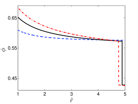
Figure 12: Equilibrium profiles $\phi(\tilde{r})$ for a closed wedge system with an average composition $\phi_{0}=0.58$ larger than $\phi_{c}$. Dashed line: $M_{{\rm w}}=1\times 10^{-3}$ smaller than $M_{{\rm w}}^{*}$, and $\phi(\tilde{r})$ is smoothly varying. Solid line: $M_{{\rm w}}=4\times 10^{-3}$ is large enough to induce phase separation. Dash-dot line: $M_{{\rm w}}=8\times 10^{-3}$, the separation interface moves to a smaller radius. We used $T=0.993T_{c}$.

Since the electric field breaks the symmetry of the free energy with respect to composition ($\phi\rightarrow 1-\phi$), the full stability diagram is asymmetric with respect to $\phi-\phi_{c}$. Fig. 11 (a) shows that in an open system, phase separation does not occur when $\phi_{0}>\phi_{c}$. In Fig. 11 (b) there are unstable compositions $\phi_{0}$ such that $\phi_{0}>\phi_{c}$. This is an important feature of the stability diagram in closed systems. Here, the dielectrophoretic force that pulls the high dielectric constant liquid toward the electrode creates a depletion in the region where electric field is low, and phase separation will occur if the composition at this region is close to the binodal composition. The stability curves in Fig. 11 (b) show that higher values of potential or charge are required for demixing when $\phi_{0}>\phi_{c}$. Indeed, the ratio of electrostatic energies at the inner and outer radii is $\simeq\tilde{R}_{2}^{2}/\tilde{R}_{1}^{2}$.

.

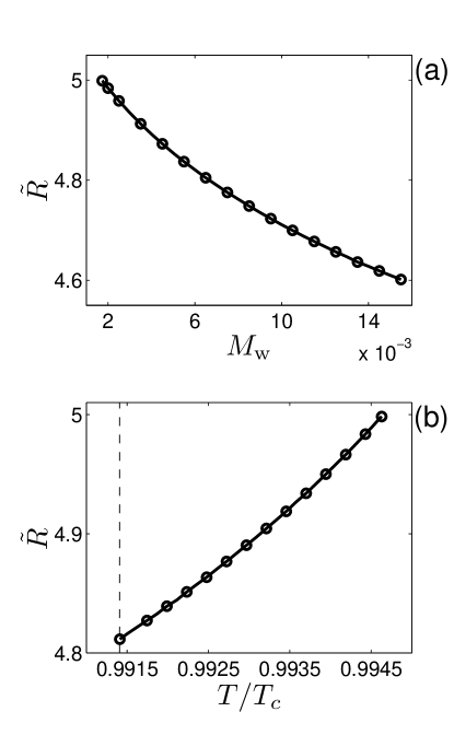
Figure 13: (a) Interface location $\tilde{R}$ for a closed wedge system with an average composition $\phi_{0}=0.58>\phi_{c}$ as a function of $M_{{\rm w}}$ at $T=0.993T_{c}$. The minimal value of $\tilde{R}$ is $\tilde{R}_{\infty}=3.86$ given by Eq. (13). (b) $\tilde{R}$ as a function of $T$ at $M_{{\rm w}}=4\times 10^{-3}$. Dashed line is $T_{t}$.

Examples of this behavior are shown in Fig. 12. When $\phi>\phi_{c}$, and $M$ is small (dashed line) $\phi(\tilde{r})$ varies smoothly, exhibiting the usual dielectrophoretic behavior. However, if $M$ is sufficiently large, that is $M>M^{*}$, the long range dielectrophoretic force gives rise to a phase-separation transition near $\tilde{R}_{2}$ (solid line). If $M$ is further increased the phase-separation interface moves to smaller radii (dash-dot line).

Fig. 13 shows how $\tilde{R}$ varies with $M$ and $T$ in the wedge geometry for $\phi>\phi_{c}$. At $M^{*}$, the interface appears where the field is minimal, i.e at $\tilde{R}_{2}=5$, see Fig. 13 (a). An increase in $M$ decreases $\tilde{R}$ and the volume of the high-$\phi$ domain. Fig. 13 (b) shows that at fixed $M$, $\tilde{R}$ decreases with $T$ and attains its minimal value at $T_{t}$. The minimal value of $\tilde{R}$ is $\tilde{R}_{\infty}$ given by Eq. (13).

When $\tilde{\varepsilon}^{\prime\prime}\neq 0$, the stability curves in Fig. 11 (b) have another kink at $\phi>\phi_{c}$ at a temperature we denote $T_{k,2}$. From the previous discussion, $T_{k,2}$ is obtained by replacing $\tilde{R}_{1}$ by $\tilde{R}_{2}$ in Eq. (24). In the wedge geometry we thus find

$$\frac{T_{k,2}}{T_{c}}=1+\frac{M_{{\rm w}}\tilde{\varepsilon}^{\prime\prime}}{\tilde{R}_{2}^{2}}.$$ (26)

Hence, $T_{c}-T_{k,2}$ is smaller than $T_{c}-T_{k,1}$ by a factor of $\tilde{R}_{2}^{2}$.

IV Conclusions

We present a systematic study of electric field induced phase-separation transitions in binary mixtures on the mean field level. The behavior described by us complements the findings of Onuki and co-workers Onuki (2006); Onuki and Kitamura (2004); Onuki and Okamoto (2009) and Ben-Yaakov et al. (2009) who mainly focused on effects above the critical temperature or on miscible liquids. The transitions should occur in any bistable system with a dielectric mismatch sufficiently close to the transition temperature, e.g a vapor phase close to coexistence with its liquid. The differences between closed and open systems and between the three geometries are highlighted. The stability diagrams in the temperature-composition plane are given. These diagrams show that the change in the transition temperature is much larger in nonuniform fields than in uniform fields. We describe the special temperatures $T_{k,1}$ and $T_{k,2}$ where the stability diagram has a “kink”. It should be emphasized that the location of the phase separation interface is not restricted to the vicinity of the confining surfaces, and can appear at a finite location $\tilde{R}$ in the range of temperatures $T_{k,1}<T<T_{k,2}$ as described above in Fig. 11. In other geometries, too, the demixing interface can be created far from any surface, e.g in quadrupolar electrode array.

In order to test our predictions we suggest the following experiments. Consider a wedge capacitor partially immersed in a binary liquid mixture near the coexistence temperature. Neutron reflectometry may be used to probe directly the composition profile Bowers et al. (2007) and to determine the critical voltage for demixing. Here we expect $\tilde{R}$ to be proportional to the voltage difference across the electrodes. A different experiment can be realized by suspending a conducting wire in a dilute vapor phase of a pure substance near the coexistence temperature with the liquid. When a potential $V$ is applied to the wire, its fundamental frequency of vibration perpendicular to its length changes from $f_{0}$ to $f_{V}$ because a liquid layer condenses around the wire. We expect that the ratio $(f_{0}/f_{V})^{2}$ should be a linear function of $V^{2}$. Alternatively, one can measure directly the change in the wire mass $\Delta m$ using a microbalance – $\Delta m$ should depend linearly on $V^{2}$. In these experiments, care must be taken to subtract wetting or confinement effects due to the electrodes.

Capillary condensation has been described Dobbs and Yeomans (1992); Bauer et al. (2000); Beysens and Estève (1985); Narayanan et al. (1993); Koehler and Kaler (1997) for colloidal suspensions in binary mixtures. According to our work, charged colloidal suspensions can flocculate or be stabilized due to the formation of liquid layers around the colloids. The liquid layer may also influence the interaction between a colloid and a flat surface both far and close to the critical point Hertlein et al. (2008).

Our results may also be measurable in Surface Force Balance and Atomic Force Microscope experiments. In such apparatus, a bridging transition has been observed in binary mixtures Wennerstrom et al. (1998) and explained by capillary forces Andrienko et al. (2004); Olsson et al. (2004). Since in most cases the surfaces are charged, a capillary bridge could be the result of the merging of two field-induced layers, leading to long range attractive forces between the surfaces.

In the current work we neglect a $(\nabla\phi)^{2}$ in the mixing free energy $f_{m}$, since the system size was relatively large and the electrostatic energy acts throughout the whole system volume, and therefore is dominant Onuki (2004b). We have verified that inclusion of such term leads to smoothing of composition profiles but otherwise to no other noticeable changes in the figures presented. In order to isolate the electric field effect, we have also not considered any direct short- or long-range interactions with the confining surfaces. In a future study it would be very interesting to relax these assumptions and to look at ever smaller systems. Here we are intrigued by the possibility to find qualitative, and not just quantitative, differences from our current profiles and diagrams.

References

- Landau and Lifshitz (1957) L. D. Landau and E. M. Lifshitz, Elektrodinamika Sploshnykh Sred Chap. II, Sec. 18, Problem 1 (Nauka, Moscow, 1957).
- Onuki (1995) A. Onuki, Europhys. Lett. 29, 611 (1995).
- Debye and Kleboth (1965) P. Debye and K. Kleboth, J. Chem. Phys. 42, 3155 (1965).
- Beaglehole (1981) D. Beaglehole, J. Chem. Phys. 74, 5251 (1981).
- Orzechowski (1999) K. Orzechowski, Chem. Phys. 240, 275 (1999).
- Wirtz and Fuller (1993) D. Wirtz and G. G. Fuller, Phys. Rev. Lett. 71, 2236 (1993).
- Reich and Gordon (1979) S. Reich and J. M. Gordon, J. Pol. Sci.: Pol. Phys. 17, 371 (1979).
- Gábor and Szalai (2008) A. Gábor and I. Szalai, Molecular Physics 106, 801 (2008), ISSN 0026-8976.
- Onuki (2006) A. Onuki, Phys. Rev. E 73, 021506 (2006).
- Schoberth et al. (2009) H. G. Schoberth, K. Schmidt, K. A. Schindler, and A. Boker, Macromolecules 42, 3433 (2009).
- Tsori et al. (2006) Y. Tsori, D. Andelman, C.-Y. Lin, and M. Schick, Macromolecules 39, 289 (2006).
- Tsori (2009) Y. Tsori, Rev. Mod. Phys. 81, 1471 (2009).
- com (a) It has been argued by Stepanow and co-workers that fluctuation effects near the critical point change this behavior Gunkel et al. (2007); Stepanow and Thurn-Albrecht (2009).
- Gunkel et al. (2007) I. Gunkel, S. Stepanow, T. Thurn-Albrecht, and S. Trimper, Macromolecules 40, 2186 (2007).
- Stepanow and Thurn-Albrecht (2009) S. Stepanow and T. Thurn-Albrecht, Phys. Rev. E 79, 041104 (2009).
- Tsori et al. (2004) Y. Tsori, F. Tournilhac, and L. Leibler, Nature 430, 544 (2004).
- Marcus et al. (2008) G. Marcus, S. Samin, and Y. Tsori, J. Chem. Phys. 129, 061101 (2008).
- Landau et al. (1984) L. D. Landau, E. M. Lifshitz, and L. P. Pitaevskii, Electrodynamics of Continuous Media (Butterworth-Heinemann, Amsterdam, 1984), 2nd ed.
- Onuki (2004a) A. Onuki, Nonlinear dielectric phenomena in complex liquids (Kluwer Academic, Dordrecht, 2004a).
- Onuki and Kitamura (2004) A. Onuki and H. Kitamura, J. Chem. Phys. 121, 3143 (2004).
- Onuki (2004b) A. Onuki, Phase transition dynamics (Cambridge University Press, 2004b).
- Doi (1996) M. Doi, Introduction to polymer physics (Oxford University Press, Oxford, UK, 1996).
- Akhadov (1981) Y. Y. Akhadov, Dielectric properties of binary solutions (Oxford : Pergamon Press, 1981).
- Sen et al. (1992) A. D. Sen, V. G. Anicich, and T. Arakelian, J. Phys. D: Appl. Phys. 25, 616 (1992).
- com (b) Strictly speaking, the spinodal compositions are “forbidden”, because the spinodal is the locus of critical points, and thus critical fluctuations are expected to be important. The current mean-field treaties therefore is not expected to hold when .
- Landau and Lifshitz (1980) L. D. Landau and E. M. Lifshitz, Statistical Physics Part 1 §144 (Butterworth-Heinemann, Amsterdam, 1980), 3rd ed.
- Onuki and Okamoto (2009) A. Onuki and R. Okamoto, J. Phys. Chem. B 113, 3988 (2009).
- Ben-Yaakov et al. (2009) D. Ben-Yaakov, D. Andelman, D. Harries, and R. Podgornik, J. Phys. Chem. B 113, 6001 (2009).
- Bowers et al. (2007) J. Bowers, A. Zarbakhsh, I. A. McLure, J. R. P. Webster, R. Steitz, and H. K. Christenson, J. Phys. Chem. C 111, 5568 (2007).
- Dobbs and Yeomans (1992) H. T. Dobbs and J. M. Yeomans, J. Phys.: Condens. Matter 4, 10133 (1992).
- Bauer et al. (2000) C. Bauer, T. Bieker, and S. Dietrich, Phys. Rev. E 62, 5324 (2000).
- Beysens and Estève (1985) D. Beysens and D. Estève, Phys. Rev. Lett. 54, 2123 (1985).
- Narayanan et al. (1993) T. Narayanan, A. Kumar, E. S. R. Gopal, D. Beysens, P. Guenoun, and G. Zalczer, Phys. Rev. E 48, 1989 (1993).
- Koehler and Kaler (1997) R. D. Koehler and E. W. Kaler, Langmuir 13, 2463 (1997).
- Hertlein et al. (2008) C. Hertlein, L. Helden, A. Gambassi, S. Dietrich, and C. Bechinger, Nature 451, 172 (2008).
- Wennerstrom et al. (1998) H. Wennerstrom, K. Thuresson, P. Linse, and E. Freyssingeas, Langmuir 14, 5664 (1998).
- Andrienko et al. (2004) D. Andrienko, P. Patricio, and O. I. Vinogradova, J. Chem. Phys. 121, 4414 (2004).
- Olsson et al. (2004) M. Olsson, P. Linse, and L. Piculell, Langmuir 20, 1611 (2004).