A Summary of Bulk Dynamics from Quark Matter 2009

Abstract

I review the recent progress in measuring elliptic flow in heavy ion collisions. These measurements show clearly how hydrodynamics starts to develop as the system size is increased from peripheral to central collisions. During this transition, the momentum range described by hydrodynamics increases as the system progresses from a kinetic to a hydrodynamic regime. Many of the systematic deviations from ideal hydrodynamics are reproduced effortlessly once the shear viscosity is included. In order to extract the shear viscosity from the data, kinetic theory can be used to determine which aspects of the elliptic flow reflect the details of the microscopic interactions, and which aspects reflect the underlying transport coefficients. I also review the identified hadron elliptic flow and the predictions of hydrodynamics for the LHC.

1 Overview

Perhaps the most important result from the Relativistic Heavy Ion Collider is the observation of strong elliptic flow [2, 3]. Elliptic flow is an asymmetry of particle production with respect to the reaction plane and has been measured as a function of transverse momentum, rapidity, and particle type. The interpretation of the observed flow which has been adopted by the heavy ion community is that the elliptic flow is the hydrodynamic response to the collision geometry. Implicit in this interpretation of the observed flow is that the time scale for momentum relaxation near the QCD phase transition is of order the quantum time scale

$$\tau_{R}\sim\frac{\hbar}{\pi T}\,.$$ (1)

This estimate for the relaxation time is best expressed in terms of the shear viscosity to entropy ratio. For instance, in the viscous Bjorken model the energy density at time $\tau_{o}$ evolves as

$$\frac{de}{d\tau}=-\frac{e+{\mathcal{P}}}{\tau_{o}}+\frac{4}{3}\frac{\eta}{\tau^{2}_{o}}\,,$$ (2)

where $e$ is the energy density, ${\mathcal{P}}$ is the pressure, and $\eta$ is the shear viscosity [4]. Comparing the size of the viscous term to the ideal term, we conclude that hydrodynamics will provide a good description of the observed flow when

$$\frac{\eta}{(e+{\mathcal{P}})\tau_{o}}\ll 1\,.$$ (3)

Using $e+{\mathcal{P}}=sT$, and an estimate for the temperature and $\tau_{o}$, this criterion reads

$$0.2\left(\frac{\eta/s}{0.3}\right)\left(\frac{1\,{\rm fm}}{\tau_{o}}\right)\left(\frac{300\,\mbox{MeV}}{T_{o}}\right)\ll 1{\,.}$$ (4)

From this estimate we see that hydrodynamics will begin to be a good approximation for $\eta/s\mbox{~{}{\raisebox{1.72218pt}{$<$}} {\raisebox{-2.58334pt}{$\sim$}}~{}}0.3$ or so. To reiterate, implicit in the hydrodynamic interpretation of the flow results is a strong conclusion about the transport coefficients of QCD.

Many of the systematic trends seen in the elliptic flow data do support the hydrodynamic interpretation of the observed flow. For example, as a function of centrality and transverse momentum, the measured elliptic flow deviates from ideal hydrodynamics in a way characteristic of viscosity. These experimental trends have been fully clarified only recently and the experimental analysis is now rather sophisticated. These developments were reported on at the Quark Matter conference and are reviewed in Section 2. The systematics of the recent flow measurements give confidence in the overall picture of the hydrodynamic expansion.

Although these experimental trends support the notion of a hydrodynamic response, there are several puzzling patterns in the elliptic flow data. For example, new data on the elliptic flow of the $\phi$ meson and the $\Omega^{-}$ baryon are reviewed in Section 2. The differences in the measured flow between mesons and baryons is generally explained with the coalescence model, which enjoys considerable phenomenological success. However, the coalescence model is theoretically unsatisfactory and is difficult to realize in a dynamical model. The seemingly simple coalescence trends seen in the elliptic flow data must be understood before the shear viscosity and other transport properties can be reliably extracted from the heavy ion data.

In addition to experimental progress, there has been substantial theoretical progress in classifying the form of viscous corrections, both with viscous hydrodynamics and with kinetic theory. A brief summary of some of the developments discussed at Quark Matter 2009 is presented in Section 3. Most of these ideas presented in this summary are reviewed more completely in Ref.[3], which was written shortly after the Quark Matter conference. Some sections from this longer review have been copied for this brief summary.

2 Measurements

One of the best ways to test the hydrodynamic interpretation is to systematically observe how the response changes from small systems to large systems. Experimentally this can be accomplished by colliding small nuclei such as CuCu and selecting peripheral collisions. Unfortunately measuring elliptic flow in these smaller systems is rather difficult, and reliable, precise results have become available only recently.

The difficulty in measuring flow in small systems stems from fluctuations. Especially in peripheral AuAu and CuCu collisions, there are fluctuations in the initial eccentricity of the participants. Thus rather than using the continuum approximation to categorize the geometry, it is better to implement a Monte-Carlo Glauber calculation and estimate the eccentricity using the “participant plane eccentricity”. This event by event eccentricity is denoted $\epsilon_{PP}$ in the literature. Clearly the experimental goal is to extract the response coefficient $C$ relating the elliptic flow to the eccentricity on an event by event basis

$$v_{2}=C\epsilon_{PP}{\,.}$$ (5)

If the flow methods measured $\left\langle v_{2}\right\rangle$, then we could simply divide the measured flow to determine the response coefficient, $C=\left\langle v_{2}\right\rangle/\left\langle\epsilon_{PP}\right\rangle$. The PHOBOS collaboration deciphered the confusing CuCu data by recognizing the need for $\epsilon_{PP}$ and following this procedure[5]. However, it was generally realized (see in particular. Ref.[6]) that the elliptic flow methods do not measure precisely $\left\langle v_{2}\right\rangle$. Some methods (such as two particle correlations $v_{2}\left\{2\right\}$) are sensitive to $\sqrt{\left\langle v^{2}_{2}\right\rangle}$, while other methods (such as the event plane method $v_{2}\left\{EP\right\}$) measure something closer to $\left\langle v_{2}\right\rangle$. What precisely the event plane method measures depends on the reaction plane resolution in a known way[7]. So just dividing the measured flow by the average participant eccentricity is not entirely correct. The appropriate quantity to divide by depends on the method [6, 8, 9]. In a Gaussian approximation for the eccentricity fluctuations this can be worked out analytically. For instance, the two particle correlation elliptic flow $v_{2}\left\{2\right\}$ (which measures $\sqrt{\left\langle v_{2}^{2}\right\rangle}$), should be divided by $\sqrt{\left\langle\epsilon_{PP}^{2}\right\rangle}{\,.}$ With a complete understanding of what each method measures, Ref.[7] was able to make a simple model for the fluctuations and non-flow and show that $\left\langle v_{2}\right\rangle$ measured by the different methods are compatible to high precision. This is illustrated in Fig. 1. The stunning precision of the recent flow measurements will be very useful in understanding how hydrodynamics begins to work in peripheral collisions. This work should be extended to the CuCu system where non-Gaussian fluctuations are stronger and ultimately corroborate the PHOBOS analysis [5, 10]. This is a worthwhile goal because it will clarify fully the transition into the hydrodynamic regime [11, 12].

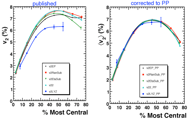
Figure 1: (a) The elliptic flow measured by different methods [7]. The methods measure different quantities and should agree only when fluctuations are neglected. (b) The average elliptic flow $\left\langle v_{2}\right\rangle$ measured by the different methods. To determine $\left\langle v_{2}\right\rangle$ for each method, non-flow was estimated using measured $pp$ data and fluctuations were estimated with a geometric model.

The scaled elliptic flow $v_{2}/\epsilon$ measures the response of the medium to the initial geometry and can be used to determine the regime of validity of hydrodynamics. Additional information about the shear viscosity can be gleaned from the transverse momentum dependence of the observed elliptic flow. Fig. 2 shows $v_{2}(p_{T})/\epsilon$ as a function of centrality, 0-5% being the most central and 60-70% being the most peripheral. Examining this figure we see a gradual transition from a weak to a strong dynamic response with growing system size. The interpretation adopted here is that this change is a consequence of a system transitioning from a kinetic to a hydrodynamic regime.

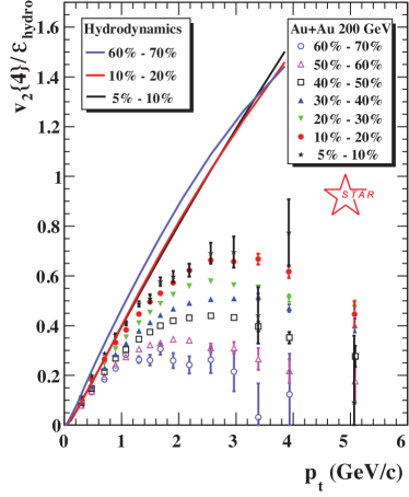
Figure 2: Elliptic flow $v_{2}(p_{T})$ as measured by the STAR collaboration [13, 14] for different centralities. The measured elliptic flow has been divided by the eccentricity. The curves are ideal hydrodynamic calculations based on Refs.[15, 16] rather than the viscous hydrodynamics discussed in much of this summary.

There are several theoretical curves based upon calculations of ideal hydrodynamics[16, 17] which for $p_{T}<1\,{\rm GeV}$ approximately reproduce the observed elliptic flow in the most central collisions. Since ideal hydrodynamics is scale invariant (for a scale invariant equation of state) the expectation is that the response $v_{2}/\epsilon$ of this theory should be independent of system size or centrality. This reasoning is borne out by the more elaborate hydrodynamic calculations shown in the figure. On the other hand, the data show a gradual transition as a function of increasing centrality, rising towards the ideal hydrodynamic calculations in a systematic way. These trends are captured by models with a finite mean free path[18].

The data show other trends as a function of centrality. In more central collisions the linearly rising trend, which resembles the ideal hydrodynamic calculations, extends to larger and larger transverse momentum. Viscous corrections to ideal hydrodynamics grow as

$$\left(\frac{p_{T}}{T}\right)^{2}\frac{\ell_{\rm\scriptscriptstyle mfp}}{L}{\,,}$$ (6)

where $L$ is a characteristic length scale. Thus these viscous corrections restrict the applicable momentum range in hydrodynamics [19]. In more central collisions, where $\ell_{\rm\scriptscriptstyle mfp}/L$ is smaller, the transverse momentum range described by hydrodynamics extends to increasingly large $p_{T}$. These qualitative trends are reproduced by the more involved viscous calculations [3].

While many of the trends seen in Fig. 1 and Fig. 2 are reproduced and understood with viscous hydrodynamics, there are additional trends in the elliptic flow data which are only partially understood. For instance Fig. 3(a) shows the elliptic flow of identified particles $\pi,K,p$. At low momenta the separation amongst the different particle species is well reproduced by hydrodynamics. However as the momentum is increased the proton elliptic flow equals, and then exceeds, the pion elliptic flow. These systematic trends are seen in all collision systems and centralities. The prevailing explanation is that constituent quarks coalesce to form hadrons at the phase boundary. This ansatz is supported by the observation that if the hadron momentum and $v_{2}$ is divided by the valence quark content all of the $v_{2}$ of the different hadron species lie along a single curve. This is illustrated in Fig. 3(b) which is plotted as a function of $KE_{T}=\sqrt{p_{T}^{2}+M^{2}}-M$ rather than transverse momentum to capture the hydrodynamic behavior at small momentum. Although constituent quark scaling works rather well, the theoretical support for quark coalescence is small since it is difficult to realize a coalescence mechanism in a dynamical simulation. It nevertheless remains to find an alternative picture for the observed different flows of mesons and baryons. At the Quark Matter conference the elliptic flow of identified particles was measured accurately out to rather large transverse momenta. At sufficiently large momenta the data deviate from a universal coalescence curve providing new insight into the hadronization dynamics in this region.

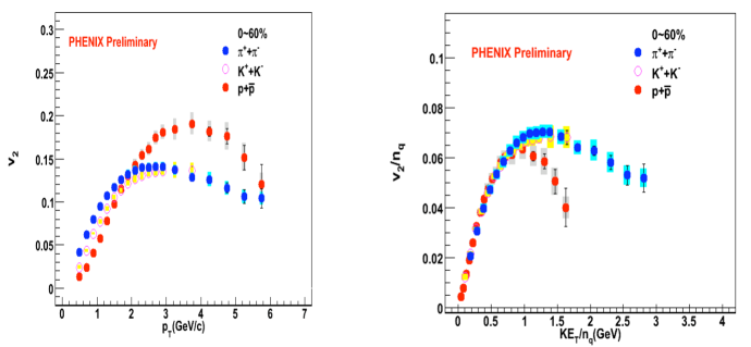
Figure 3: (a) The elliptic flow as a function of transverse momentum for identified particles as measured by the PHENIX collaboration [20]. (b) The elliptic flow of identified hadrons rescaled according to the quark coalescence model and plotted as a function of $KE_{T}=\sqrt{p_{T}^{2}+M^{2}}-M$.

To conclude this section, we turn to Fig. 4 which compares the elliptic flow protons and pions to the flow of the multi-strange hadrons $\Omega^{-}$ and $\phi$. The important point is that the $\Omega^{-}$ is nearly twice as heavy as the proton and more importantly, does not have a strong resonant interaction analogous to the $\Delta$. For these reasons the hadronic relaxation time of the $\Omega^{-}$ is expected to be much longer than the duration of the heavy ion event. Nevertheless the $\Omega^{-}$ shows nearly the same elliptic flow as the protons. This provides fairly convincing evidence that the majority of the elliptic flow develops during a deconfined phase which hadronizes to produce a flowing $\Omega^{-}$ baryon.

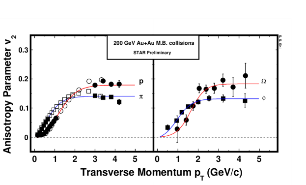
Figure 4: A comparison of the elliptic flow of pions and protons to the elliptic flow of the multi-strange $\phi$ and $\Omega^{-}$ [21].

3 Modeling Elliptic Flow with Hydrodynamics and Kinetic Theory

Many of the trends seen in the data (with the possible exception of quark coalescence) are reproduced by hydrodynamics and kinetic theory. Generally the kinetic theory estimates for the shear viscosity are consistent with the estimates from viscous hydrodynamics. Specifically unless $\eta/s\mbox{~{}{\raisebox{1.72218pt}{$<$}} {\raisebox{-2.58334pt}{$\sim$}}~{}}0.3$ it is impossible to reproduce the observed elliptic flow. Given that the transport time scales extracted from the heavy ion data are close to the quantum time scale given in Eq. (1), it is clear that the microscopic details of kinetic models cannot be trusted. Nevertheless these shortcomings of the microscopic theory are unimportant in the hydrodynamic regime. In the hydrodynamic regime the only properties that determine the evolution of the system are the equation of state, ${\mathcal{P}}(e)$, and the shear viscosity and bulk viscosities, $\eta(e)$ and $\zeta(e)$. In the sense that kinetic theory provides a reasonable guess as to how the surface to volume ratio influences the forward evolution, these models can be used to estimate the shear viscosity, and the estimate may be more reliable than the hydrodynamic models. More importantly, by comparing the results of different microscopic models one can determine which features of the heavy ion data are universal ($i.e.$ only depend on $\eta(e),{\mathcal{P}}(e)$ and $\zeta(e)$ ).

There were a number of promising efforts to reproduce hydrodynamic results from kinetic theory reported at the conference. First there was an effort to reproduce hydrodynamic shocks with kinetic theory by the Frankfurt group. Fig. 5(a) shows a kinetic theory simulation of the shock tube problem. Clearly the BAMPS code is capable of reproducing the correct hydrodynamic limit in detail. The deviations of the BAMPS code from ideal hydro are beautifully reproduced by viscous hydro. This gives a great deal of confidence in the BAMPS code and in the viscous hydrodynamic code vSHASTA. Additional results from the BAMPS simulation of elliptic flow were presented in the poster session.

A similar approach to the hydrodynamic limit was reported by Huovinnen and Molnar [22], and Gombeaud [12]. In particular Fig. 5(b) shows a simulation of the MPC code which also makes a direct comparison with viscous hydrodynamics for the Bjorken expansion of an ideal massless gas with constant cross section. As the Knudsen number $K\equiv\sigma/\pi R^{2}\,dN/dy$ is increased, the simulation approaches Israel-Stewart hydro and ultimately the Navier-Stokes limit. Given that the kinetic code and the viscous hydrodynamic simulations agree reasonably, the MPC code can be used to reliably extract the shear viscosity from the heavy ion data.

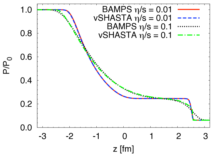
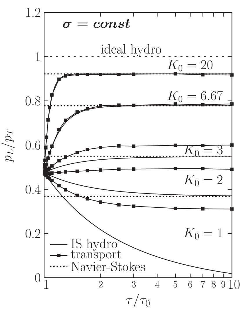
Figure 5: (a) The pressure relative to the initial pressure for shock tube initial conditions. The three curves are for the BAMPS parton cascade model, viscous hydrodynamics (vSHASTA), and ideal hydrodynamics [23]. (b) The ratio of longitudinal and transverse pressures in kinetic theory, Israel Stewart hydrodynamics, and the Navier-Stokes equations, for a Bjorken expansion of a massless ideal gas with constant cross section. The simulations are compared as a function of Knudsen number, $K\equiv\sigma/\pi R^{2}\,dN/dy$ [22].

When viscous hydrodynamics is extended to a second order there are additional relaxation times (e.g. $\tau_{\pi}$) beyond the shear viscosity, $\eta(e)$. Just as transport models should be approximately independent of the details of the microscopic interactions, results from viscous hydrodynamics should be approximately independent of the precise way in which the second order terms are implemented. This is indeed the case [24, 25, 26]. Additional results from viscous hydrodynamics will be discussed more completely by P. Romatschke in this volume [27].

4 Outlook

Clearly there is a strong convergence between kinetic and hydrodynamic simulations of heavy ion reactions. These simulations reproduce many trends observed in increasingly precise measurements of elliptic flow. This convergence strongly suggests that the hydrodynamic interpretation of the observed flow is correct. One of the striking tests of hydrodynamic predictions is the saturation of elliptic flow at high energy. From RHIC to the LHC, hydrodynamics predicts an increase in the flow which is significantly less than a naive extrapolation from lower energies. This is illustrated in Fig. 6 and will be one of the first tests of the hydrodynamic paradigm at the LHC.

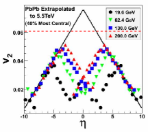
Figure 6: Figure presented by W. Busza providing an estimate for the elliptic flow at the LHC by extrapolating trend lines from lower energy to higher energy (solid black lines) [28]. The dashed red lines shows an estimate based on ideal hydrodynamics [29].

References

- [1]
- [2] See for example, S. A. Voloshin, A. M. Poskanzer and R. Snellings, arXiv:0809.2949 [nucl-ex].
- [3] D. A. Teaney, “Viscous Hydrodynamics and the Quark Gluon Plasma,” arXiv:0905.2433 [nucl-th]; prepared for “Quark-gluon plasma. Vol. 4,” eds. R.C. Hwa, X.N. Wang.
- [4] P. Danielewicz and M. Gyulassy, Phys. Rev. D 31, 53 (1985).
- [5] B. Alver et al. [PHOBOS Collaboration], Phys. Rev. Lett. 98, 242302 (2007) [arXiv:nucl-ex/0610037].
- [6] M. Miller and R. Snellings, “Eccentricity fluctuations and its possible effect on elliptic flow arXiv:nucl-ex/0312008.
- [7] A. .M .Poskanzer, theser proceedings; see also J. Y. Ollitrault, A. M. Poskanzer and S. A. Voloshin, arXiv:0904.2315 [nucl-ex].
- [8] R. S. Bhalerao and J. Y. Ollitrault, Phys. Lett. B 641, 260 (2006) [arXiv:nucl-th/0607009].
- [9] S. A. Voloshin, A. M. Poskanzer, A. Tang and G. Wang, Phys. Lett. B 659, 537 (2008) [arXiv:0708.0800 [nucl-th]].
- [10] B. Alver et al., Phys. Rev. C 77, 014906 (2008) [arXiv:0711.3724 [nucl-ex]].
- [11] H. J. Drescher, A. Dumitru, C. Gombeaud and J. Y. Ollitrault, Phys. Rev. C 76, 024905 (2007) [arXiv:0704.3553 [nucl-th]].
- [12] C. Gombeaud these proceedings; see also C. Gombeaud, T. Lappi and J. Y. Ollitrault, arXiv:0907.1392 [nucl-th].
- [13] The data presented are from the thesis Dr. Yuting Bai.
- [14] See for example, B. I. Abelev et al. [STAR Collaboration], Phys. Rev. C 77, 054901 (2008) [arXiv:0801.3466 [nucl-ex]].
- [15] P. Huovinen and P. V. Ruuskanen, Ann. Rev. Nucl. Part. Sci. 56, 163 (2006) [arXiv:nucl-th/0605008].
- [16] P. Huovinen, P. F. Kolb, U. W. Heinz, P. V. Ruuskanen and S. A. Voloshin, Phys. Lett. B 503, 58 (2001) [arXiv:hep-ph/0101136].
- [17] P. F. Kolb, P. Huovinen, U. W. Heinz and H. Heiselberg, Phys. Lett. B 500, 232 (2001) [arXiv:hep-ph/0012137].
- [18] H. J. Drescher, A. Dumitru and J. Y. Ollitrault, arXiv:0706.1707 [nucl-th]; in N. Armesto et al., “Heavy Ion Collisions at the LHC - Last Call for Predictions,” J. Phys. G 35, 054001 (2008).
- [19] D. Teaney, Phys. Rev. C 68, 034913 (2003) [arXiv:nucl-th/0301099].
- [20] A. Taranenko for the PHENIX Collaboration, these proceedings; see also A. Adare et al. [PHENIX Collaboration], Phys. Rev. Lett. 98, 162301 (2007) [arXiv:nucl-ex/0608033].
- [21] S. Shi for the STAR Collaboration, arXiv:0907.2265 [nucl-ex].
- [22] P. Huovinen and D. Molnar, Phys. Rev. C 79, 014906 (2009) [arXiv:0808.0953 [nucl-th]].
- [23] I. Bouras et al., Phys. Rev. Lett. 103, 032301 (2009) [arXiv:0902.1927 [hep-ph]].
- [24] M. Luzum and P. Romatschke, Phys. Rev. C 78, 034915 (2008) [arXiv:0804.4015 [nucl-th]].
- [25] K. Dusling and D. Teaney, Phys. Rev. C 77, 034905 (2008) [arXiv:0710.5932 [nucl-th]].
- [26] H. Song and U. W. Heinz, Phys. Rev. C 77, 064901 (2008) [arXiv:0712.3715 [nucl-th]].
- [27] P. Romatschke, these proceedings; see also Ref.[24].
- [28] W. Busza these proceedings, arXiv:0907.4719 [nucl-ex].
- [29] D. Teaney, J. Lauret and E. V. Shuryak, arXiv:nucl-th/0110037. ibid, Phys. Rev. Lett. 86, 4783 (2001)