Assault on the NLO Wishlist: $pp\rightarrow t\bar{t}b\bar{b}$

Abstract:

We present the results of a next-to-leading order calculation of QCD corrections to the production of an on-shell top-anti-top quark pair in association with two flavored b-jets. Besides studying the total cross section and its scale dependence, we give several differential distributions. Where comparable, our results agree with a previous analysis. While the process under scrutiny is of major relevance for Higgs boson searches at the LHC, we use it to demonstrate the ability of our system built around Helac-Phegas to tackle complete calculations at the frontier of current studies for the LHC. On the technical side, we show how the virtual corrections are efficiently computed with Helac-1Loop, based on the OPP method and the reduction code CutTools, using reweighting and Monte Carlo over color configurations and polarizations. As far as the real corrections are concerned, we use the recently published Helac-Dipoles package. In connection with improvements of the latter, we give the last missing integrated dipole formulae necessary for a complete implementation of phase space restriction dependence in the massive dipole subtraction formalism.

1 Introduction

Rare are processes, which received more attention than top quark pair production in various configurations at hadron colliders. Indeed, there is astonishing recent progress in next-to-leading order (NLO) [1, 2] and next-to-next-to leading order (NNLO) [3, 4, 5, 6, 7, 8, 9, 10] calculations, as well as next-to-next-to-leading-log resummations (NNLL) [11, 12, 13] for inclusive production. For this publication, however, we will mostly be interested in more exclusive channels. The list for the latter is just as impressive: NLO QCD corrections for the $t\bar{t}H$ signal [14, 16, 15, 17, 18, 19] and the backgrounds from $t\bar{t}j$ [20, 21], $t\bar{t}Z$ [22], $t\bar{t}b\bar{b}$ [23, 24], and most recently $t\bar{t}\gamma$ [25].

The present study pertains to the $t\bar{t}b\bar{b}$ final state. As phenomenological motivation, we stress its relevance as irreducible background for light Higgs boson searches in the $t\bar{t}H$ channel, when the Higgs boson decays into a pair of b quarks. Indeed, realistic experimental analyses of this channel [26] including showering effects, b-tagging efficiencies and suitable cuts to reduce multijet backgrounds (among others $t\bar{t}jj$ with light jets misidentified as b-jets), show a substantial smearing of what would be a sharp Higgs resonance peak in the distribution of the invariant mass of the $b\bar{b}$ system. In consequence, the knowledge of the backgrounds becomes crucial to claim discovery or exclusion. The dominant background is obviously direct production of the final state without resonances, i.e. the QCD generated process $pp\rightarrow t\bar{t}b\bar{b}+X$. As mentioned above, the NLO computation has been completed only very recently in [24]. Our first goal is to confirm the results of that publication.

The second aim is to demonstrate the power of our system based on Helac-Phegas [27, 28, 29], Helac-1Loop [30], CutTools [31, 32] and Helac-Dipoles [33] in a realistic computation with six external legs and massive partons. This is the first calculation at this level of complexity using the OPP reduction technique [31, 34] and modern unitarity based methods [35, 36, 37, 38, 39, 40, 41]. Indeed, computations with six external legs have only been attempted with massless partons [42, 43, 44], whereas massive partons have only appeared in a more modest setting in [2]. It is fair to say, that traditional, reduction based methods, have proven more efficient in producing complete results until this point (see some recent examples [45, 46, 47, 48, 49, 50, 51, 24, 52]).

In principle, the publication [30] has shown that the difficult virtual corrections can be computed within the Helac-1Loop/CutTools framework for a multitude of processes of practical interest, and $t\bar{t}b\bar{b}$ in particular. Nevertheless, it is one thing to compute a value for a single phase space point, and another to provide arbitrary differential distributions. Here we wish to convince the skeptics that the latter exercise can be mastered as well. As our title suggests, we are confident that we can now tackle any calculation from the “NLO Wishlist” [53].

Besides the virtual corrections, the calculation of the real radiation contributions is not an easy task either. Despite the announcement of several automates for Catani-Seymour [54, 55] dipole subtraction [56, 57, 58, 59, 33], the only complete and publicly available tool is Helac-Dipoles [33] (besides possibly Sherpa [56], which should become publicly available soon). In this work, we slightly increase its flexibility by allowing for phase space restriction [60, 61] in the integrated dipoles for the general massive case (most formulae were known from [62, 63]).

This publication is structured as follows. In the next section, we discuss the details of the techniques used for the evaluation of the virtual and real corrections. Subsequently, we give the results for the total cross sections and differential distributions, and conclude the main part of the text. The Appendix contains the formulae of the massive dipole formalism with phase space restriction.

2 Technicalities

2.1 Virtual corrections

For the calculation of virtual corrections we use Helac-1Loop [30], namely the merging of Helac [27, 28, 29] and the OPP [31, 34] reduction code CutTools [32]. In order to further improve the performance and speed of the system, we make use of color, helicity and event sampling methods.

The treatment of the color degrees of freedom in Helac is based on the color-connection representation of the amplitude. A generic QCD amplitude composed by $n_{g}$ gluons and $n_{q}$ quarks (and of course $n_{q}$ antiquarks) plus possible colorless particles can be written as

$${\cal M}^{i_{1}\ldots,i_{n_{q}},a_{1},\ldots,a_{n_{g}}}_{j_{1}\ldots,j_{n_{q}}}\;,$$ (1)

where $i$ and $j$ are color indices belonging to the fundamental representation of the gauge group, whereas $a$ belongs to the adjoint. Multiplying with $t^{a}_{i,j}$ and summing over $a$, for each gluon, we end up with a uniform representation, namely

$${\cal M}^{i_{1}\ldots,i_{n_{q}+n_{g}}}_{j_{1}\ldots,j_{n_{q}+n_{g}}}\;.$$ (2)

As it is well known, the amplitude can now be (color-)decomposed as follows

$${\cal M}_{j_{1},j_{2},\ldots,j_{k}}^{i_{1},i_{2},\ldots,i_{k}}=\sum_{\sigma}\delta_{i_{\sigma_{1}},j_{1}}\delta_{i_{\sigma_{2}},j_{2}}\ldots\delta_{i_{\sigma_{k}},j_{k}}A_{\sigma}\;,$$ (3)

with $k=n_{q}+n_{g}$, and $\sigma$ denoting a permutation of the set $\{1,\ldots,k\}$. The Feynman rules that allow the calculation of all $A_{\sigma}$ color-stripped amplitudes in the color-connection representation have been described in Refs. [27, 28, 29]. The objects we are interested in, are the squared matrix element

$$\sum_{\{i\},\{j\}}|{\cal M}_{j_{1},j_{2},\ldots,j_{k}}^{i_{1},i_{2},\ldots,i_{k}}|^{2}\;,$$ (4)

for tree order calculations, and

$$\sum_{\{i\},\{j\}}\{{\cal M}_{j_{1},j_{2},\ldots,j_{k}}^{i_{1},i_{2},\ldots,i_{k}}{\cal L}_{j_{1},j_{2},\ldots,j_{k}}^{*i_{1},i_{2},\ldots,i_{k}}+{\cal L}_{j_{1},j_{2},\ldots,j_{k}}^{i_{1},i_{2},\ldots,i_{k}}{\cal M}_{j_{1},j_{2},\ldots,j_{k}}^{*i_{1},i_{2},\ldots,i_{k}}\}\;,$$ (5)

for the virtual corrections, where ${\cal L}$ refers to the one-loop amplitude.

The color sum can also be written as

$$\sum_{\{i\},\{j\}}|{\cal M}_{j_{1},j_{2},\ldots,j_{k}}^{i_{1},i_{2},\ldots,i_{k}}|^{2}=\sum_{\sigma,\sigma^{\prime}}A^{*}_{\sigma}{\cal C}_{\sigma,\sigma^{\prime}}A_{\sigma^{\prime}}\;.$$ (6)

The color matrix used above is given by

$${\cal C}_{\sigma,\sigma\prime}\equiv\sum_{\{i\},\{j\}}\delta_{i_{\sigma_{1}},j_{1}}\delta_{i_{\sigma_{2}},j_{2}}\ldots\delta_{i_{\sigma_{k}},j_{k}}\delta_{i_{\sigma^{\prime}_{1}},j_{1}}\delta_{i_{\sigma^{\prime}_{2}},j_{2}}\ldots\delta_{i_{\sigma^{\prime}_{k}},j_{k}}\;,$$ (7)

and is equal to

$${\cal C}_{\sigma,\sigma^{\prime}}=N_{c}^{m(\sigma,\sigma^{\prime})}\;,$$ (8)

where $m(\sigma,\sigma^{\prime})$ count the number of common cycles of the two permutations, and $N_{C}$ is the number of colors of the fundamental representation of the gauge group (three in our case).

Full color summation is performed in Helac by using the right-hand side of Eq. 6. The code generates all possible permutations of the color indices, each of them being one color connection. For each of the latter, using the color-connection Feynman rules, Helac calculates the corresponding $A_{\sigma}$ color-stripped amplitude and at the end, using Eq. 6, provides the fully color summed contribution.

Although at tree order, practical applications are fast enough with full color summation, at the one-loop level, one would opt for Monte-Carlo sampling over colors. This is done using the left-hand side of Eq. 6. The idea is rather simple [64, 65]: we generate a color configuration by assigning explicit colors to the external particles. Using the labels $1,2,3$ for the three colors in the case of QCD, a possible color assignment for a process like $g(i_{1},j_{1})g(i_{2},j_{2})\to t(i_{3},0)\bar{t}(0,j_{3})b(i_{4},0)\bar{b}(0,j_{4})$ can be $(i_{1},\ldots,i_{4})=(1,2,3,3)$ and $(j_{1},\ldots,j_{4})=(3,2,1,3)$, that is ${\cal M}^{1,2,3,3}_{3,2,1,3}$ in Eq. 2. Of course, color conservation requires that the number of times a color appears in the list of color indices ($i$), should be equal to the number of times it appears also in the list of anti-color indices ($j$).

If one now uses Eq. 3, it is easy to see that only a few of the $A_{\sigma}$ amplitudes contribute to a given color assignment. This means that including the color degree of freedom in our Monte-Carlo integration, we may reduce drastically the average number of color connections that are actually needed. For instance in the calculation of $gg\to t\bar{t}b\bar{b}$, the average number of color connections used in a Monte-Carlo sampling over color assignments, is approximately $3$ per event, resulting to almost an order of magnitude reduction in computation time with respect to the non sampling treatment, where all color connections, $24$ in that case, have to be calculated per event. This is particularly important for one-loop amplitudes. It should be emphasized that Monte-Carlo over colors is not an approximation, it is an exact treatment of the color degrees of freedom. We have extensively tested that it produces the same results as the usual full color sum of Eq. 6, see also a previous work [66].

The sampling over helicity is well described in Refs. [67, 68]. It results to a drastic improvement in speed, since only one (random) helicity configuration has to be calculated per event, whereas in the case for instance of $gg\to t\bar{t}b\bar{b}$ a full summation over helicity configurations will slow down the calculation by a factor that is approximately equal to the number of helicity configurations, namely $32$ in that case.

Finally the actual calculation of the virtual corrections is organized using a re-weighting technique  [69, 70]. To explain how this works, let us start with the following equation

$$\sigma^{LO+V}_{ab}=\int dx_{1}dx_{2}d\Phi_{m}f_{a}(x_{1})f_{b}(x_{2})\left(|{\cal M}|^{2}+{\cal M}{\cal L}^{*}+{\cal M}^{*}{\cal L}\right)\;,$$ (9)

which gives the sum of leading order (LO) and virtual (V) contributions for a scattering $ab\to m$-particles. It can be re-written as

$$\sigma^{LO+V}_{ab}=\int dx_{1}dx_{2}d\Phi_{m}f_{a}(x_{1})f_{b}(x_{2})|{\cal M}|^{2}\left(1+\frac{{\cal M}{\cal L}^{*}+{\cal M}^{*}{\cal L}}{|{\cal M}|^{2}}\right)\;.$$ (10)

Since ${\cal L}$ is a time consuming function one would like to calculate it as few times as possible. To this end a sample of un-weighted events is produced based on the tree order distribution, namely

$$g(\vec{X})\equiv g(x_{1},x_{2},\Phi_{m})=\frac{1}{\sigma^{LO}}\frac{d\sigma^{LO}_{ab}}{dx_{1}dx_{2}d\Phi_{m}}\;,$$ (11)

satisfying $\int d\vec{X}g(\vec{X})=1$. The sample $S$ of un-weighted events has the following property,

$$\frac{1}{N_{S}}\sum_{i\in S}{\cal O}(\vec{X}_{i})=\int d\vec{X}g(\vec{X})O(\vec{X})\;,$$ (12)

where the equality should be understood in the statistical sense, and ${\cal O}(\vec{X})$ is any well-defined function over the integration space. Now it is trivial to see that if

$${\cal O}(\vec{X})=\left(1+\frac{{\cal M}{\cal L}^{*}+{\cal M}^{*}{\cal L}}{|{\cal M}|^{2}}\right)\;,$$ (13)

then

$$\frac{1}{N_{S}}\sum_{i\in S}{\cal O}(\vec{X}_{i})=\frac{\sigma^{LO+V}_{ab}}{\sigma^{LO}_{ab}}\;.$$ (14)

In practice the sample of tree order un-weighted events includes all information on the integration space, namely, the color assignment, the (random)helicity configuration, the fractions $x_{1}$ and $x_{2}$ and the $m-$body phase-space. For future convenience it is produced in a standard Les Houches format [71]. One-loop contributions are only calculated for this sample of un-weighted events, and the weight assigned to each of those events is given by

$$w=\frac{{\cal M}{\cal L}^{*}+{\cal M}^{*}{\cal L}}{|{\cal M}|^{2}}\;.$$ (15)

The total virtual contribution can now be easily estimated by

$$\sigma^{V}=\left<w\right>\sigma^{B}\;,$$ (16)

where $\sigma^{B}$ is the born cross section, already included in the Les Houches file. Moreover, the sample of events including the information on $w$, can be used to produce any kinematical distribution, according to the Eq. 12.

In our application, the speed-up factor obtained in this way varies between $10^{2}$ and $10^{3}$. In fact, an event in the gluon-gluon channel costs about a second on a 3 GHz machine, and few permille level cross sections are obtained by re-weighting about fifty thousand events. The smooth distributions of the next sections are obtained on samples of two hundred thousand events. We stress it for the non-expert reader that all timings are subject to drastic future improvement, but it is easy to see that the complete calculation of the virtual corrections is a matter of one or two days on a single machine. We consider this a practical proof of the power of our approach.

Finally, for the expert reader this time, we stress that the numerical stability of the virtual correction evaluation is checked by performing a gauge independence test on each event.

2.2 Real radiation

The real radiation contribution to the process is obtained using the Catani-Seyour dipole subtraction method [54] in the massive version as described in [55] and extended for arbitrary polarizations in [33]. We use a phase space restriction on the contribution of the dipoles as originally proposed in [60, 61]. Most of the formulae needed beyond that work to account for massive partons have been presented in [62, 63]. In fact, the only missing integrated dipoles correspond to the final emitter and final spectator case, when both are massive. This situation occurs in our calculation, when a top quark emits a soft gluon, which is then absorbed by the anti-top-quark acting as the spectator of the Catani-Seymour formalism. As advertised in the introduction, we give the complete set of expressions in the most general case in the Appendix. Let us stress at this point, that, similarly to most authors, we do not use finite dipoles regularizing the quasi-collinear divergence induced by both top quarks moving in the same direction, even though they are implemented in the software. Due to the large top quark mass, they are not needed to improve the numerical convergence.

At this point let us remind the reader that the phase space restriction on the dipole phase space is defined differently depending on whether the spectator and emitter are in the final or initial states. To be more specific a given dipole contributes as follows

1. for final-final dipoles, if

   $$y_{ij,k}<\alpha_{max}^{FF}\;,$$ (17)

   where

   $$y_{ij,k}=\frac{p_{i}p_{j}}{p_{i}p_{j}+p_{i}p_{k}+p_{j}p_{k}}\;,$$ (18)

   and $p_{i},p_{j}$ and $p_{k}$ are the momenta of the emitter pair and of the spectator respectively.

2. for final-initial dipoles, if

   $$1-x_{ij,a}<\alpha_{max}^{FI}\;,$$ (19)

   where

   $$x_{ij,a}=\frac{p_{a}p_{i}+p_{a}p_{j}-p_{i}p_{j}+\frac{1}{2}(m_{ij}^{2}-m_{i}^{2}-m_{j}^{2})}{p_{a}p_{i}+p_{a}p_{j}}\;,$$ (20)

   and $p_{i},p_{j}$ and $p_{a}$ are the momenta of the emitter pair and of the spectator respectively. $m_{ij}$ is the emitter particle mass.

3. for initial-final dipoles, if

   $$u_{i}<\alpha_{max}^{IF}\;,$$ (21)

   where

   $$u_{i}=\frac{p_{i}p_{a}}{p_{i}p_{a}+p_{j}p_{a}}\;,$$ (22)

   and $p_{a},p_{i}$ are the emitter pair momenta, with $p_{a}$ in the initial state, and $p_{j}$ is the final state spectator momentum.

4. for initial-initial dipoles, if

   $${\tilde{v}}_{i}\equiv\frac{p_{a}p_{i}}{p_{a}p_{b}}<\alpha_{max}^{II}\;,$$ (23)

   where $p_{a},p_{i}$ are the emitter pair momenta, with $p_{a}$ in the initial state, and $p_{b}$ is the initial state spectator momentum.

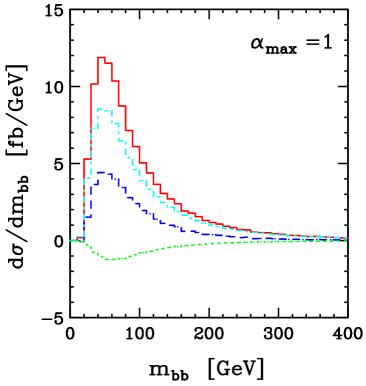
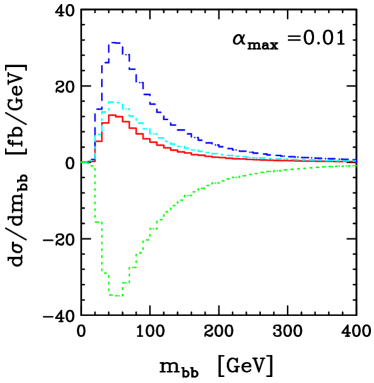
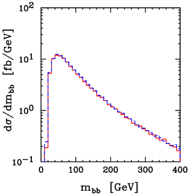
Figure 1: Distribution of the invariant mass $m_{b\bar{b}}$ of the bottom-anti-bottom pair for $pp\rightarrow t\bar{t}b\bar{b}+X$ at the LHC for different parts of the real radiation contribution with different choices of $\alpha_{max}$, $\alpha_{max}=1$ and $\alpha_{max}=0.01$. The red solid line corresponds to the sum of all contributions, the blue dashed line represents the dipole subtracted real emission, the cyan dot-dashed line corresponds to the sum of the $K$ and $P$ insertion operators, and finally the green dotted line represents the $I$ insertion operator. The sum of all the contributions for the two different choices of $\alpha_{max}$ is depicted below.

In our implementation of the subtracted real radiation the $\alpha$ parameters can be varied independently of each other. On the other hand, we slightly simplified the implementation of the integrated dipoles by assuming $\alpha_{max}^{FF}=\alpha_{max}^{FI}=\alpha_{max}^{IF}=\alpha_{max}^{II}\equiv\alpha_{max}$. We consider two extreme choices, namely $\alpha_{max}=1$ and $\alpha_{max}=0.01$. The first one corresponds of course to the original formulation of [55].

Even though the use of a phase space restriction in the dipole formalism is rather widespread currently, we wish to make a few remarks on its advantages and disadvantages in the present setting. On the side of advantages there are in fact three reasons

1. Our phase space generator, Phegas [72], uses multi-channel optimization [73], where the phase space density of a given channel corresponds to a product of Feynman diagram denominators elevated to some arbitrary power, which turned out to be best chosen relatively close to unity. This clearly reproduces the peaked behavior in the collinear and soft limits, with the integrable square root singularity after dipole subtraction. On the other hand, the distortion of the remaining (non-singular, but nevertheless present) peaks in the dipole subtraction terms due to phase space remapping is not taken into account at all. Therefore, restricting the kinematics to regions very close to the singular limits keeps the distortion small and allows to obtain a maximum gain from the available channels.

2. In close relation to the previous issue, we observe that there is more than a factor of three less events accepted if the phase space restriction parameter $\alpha_{max}$ is equal to $0.01$. The difference is due to the fact, that after phase space remapping, an event which would not be accepted by real radiation cuts, may pass the cuts of the dipole jet function if $\alpha_{max}=1$. This phenomenon is called missed-binning. It is important to note that despite more accepted events, the absolute error of the final result is only slightly better than for $\alpha_{max}=0.01$. In fact, to obtain the same absolute error, about twice less events are needed with the latter choice. This is is one of the two speed-up factors.

3. On the average much less dipole subtraction terms are needed per event with $\alpha_{max}=0.01$, since the collinear limit singles out a pair of partons, and the soft limit requires the sum over all dipoles involving the soft parton as emitter only. This constitutes the second speed-up factor.

Unfortunately, having $\alpha_{max}=0.01$ implies large cancellations between the dipole subtracted real radiation and the integrated dipole contribution. With this choice of $\alpha_{max}$, the former overshoots the complete result by a factor of almost three. It is probably safe to state that a slightly larger value of $\alpha_{max}$, such that the real radiation contribution (subtracted with dipoles) would be similar in value to the final result for the sum of real radiation and integrated dipoles, would be more advantageous. We leave this issue to future studies.

It is interesting to observe the different contributions on a chosen distribution. We illustrate such a decomposition in Fig. 1, for the invariant mass of the $b\bar{b}$ system. All parameters and cuts are defined in the next section. We separate the contribution of the $I$ operator and of the sum of the $K$ and $P$ operators defined in [55]. When introducing the $\alpha_{max}$ parameter dependence, we have again some freedom, and we choose our operators such, that the dependence of the $I$ operator is exactly as in the massless case of [61], except for the final-final integrated dipoles for which we give the formulae in the Appendix. Clearly, the mentioned large cancellations for $\alpha_{max}=0.01$ involve all three contributions, but the integrated dipoles prove to have much better convergence and the final error is entirely dominated by the statistically demanding real radiation. The plot corresponding to the sum of all contributions, also presented in Fig. 1, proves the agreement between the results for the two parameter choices. We will show the agreement on the total cross sections in the next section.

3 Results

We consider the process $pp\rightarrow t\bar{t}b\bar{b}+X$ at the LHC, i.e. for $\sqrt{s}=14$ TeV. For the top-quark mass we take $m_{t}=172.6$ GeV, whereas all other QCD partons including b quarks are treated as massless. Mass renormalization is performed in the on-shell scheme. All final-state b quarks and gluons with pseudorapidity $|\eta|<5$ are recombined into jets with separation $\sqrt{\Delta\phi^{2}+\Delta y^{2}}>D=0.8$ in the rapidity– azimuthal-angle plane via the IR-safe $k_{T}$-algorithm [74, 75, 76]. Moreover, we impose the following additional cuts on the transverse momenta and the rapidity of two recombined b-jets: $p_{T,b}>20$ GeV, $|y_{b}|<2.5$. The outgoing (anti)top quarks are neither affected by the jet algorithm nor by phase-space cuts. The separation between the b-jets, $\Delta R_{b\bar{b}}>D$, implied by the jet algorithm, together with the requirement of having both b-jets with $p_{T,b}>20$ GeV sets an effective lower limit on the invariant mass $m_{b\bar{b}}$

$$(m_{b\bar{b}})_{min}=(p_{T,b})_{min}\sqrt{2(1-\cos D)}\approx 15.6~{}\mbox{GeV}\;,$$ (24)

which screens off the collinear singularity. This is the reason, why we don’t need any dipoles for the gluon splitting into a $b\bar{b}$ pair.

We consistently use the CTEQ6 set of parton distribution functions (PDFs) [77, 78] , i.e. we take CTEQ6L1 PDFs with a 1-loop running $\alpha_{s}$ in LO and CTEQ6M PDFs with a 2-loop running $\alpha_{s}$ in NLO, but the suppressed contribution from b quarks in the initial state has been neglected. The number of active flavors is $N_{F}=5$, and the respective QCD parameters are $\Lambda^{LO}_{5}=165$ MeV and $\Lambda^{MS}_{5}=226$ MeV. In the renormalization of the strong coupling constant, the top-quark loop in the gluon self-energy is subtracted at zero momentum. In this scheme the running of $\alpha_{s}$ is generated solely by the contributions of the light-quark and gluon loops. By default, we set the renormalization and factorization scales, $\mu_{R}$ and $\mu_{F}$, to the common value $\mu_{0}=m_{t}$.

We would like to stress that the above parameters correspond exactly to those assumed in the analysis of [23, 24], and are essentially based on [26]. It is clear that there are many interesting phenomenological analyses that can be performed using our system with different cuts, but, as explained in the introduction, our main goal is to demonstrate its correctness and efficiency. To this end we want to be able to compare with the previous study.

We begin our presentation of the final results of our analysis with a discussion of the total cross section at the central value of the scale, $\mu_{R}=\mu_{F}=m_{t}$. The respective numbers are presented in Tab. 1 for the two choices of the $\alpha_{max}$ parameter. We also single out the quark channel (although its contribution beyond leading order is negligible for any practical study) because we can compare our results with [23]. Clearly, we observe perfect agreement within statistical errors between all independent evaluations. Notice that we quote smaller statistical errors than [24] for the complete proton-proton scattering cross section, mostly because we performed many experimental computations of the different sub-parts and the accumulated statistical sample is fairly sizable. At the central scale value, the full cross section receives a very large NLO correction of the order of 77% which is mainly due to the gluonic initial state as stressed previously in [24].

Process	$\sigma^{\mbox{\footnotesize{LO}}}_{\mbox{\footnotesize{\cite[cite]{[\@@bibref{}{Bredenstein:2008zb,Bredenstein:2009aj}{}{}]}}}}$ [fb]	$\sigma^{\mbox{\footnotesize{LO}}}$ [fb]	$\sigma^{\mbox{\footnotesize{NLO}}}_{\mbox{\footnotesize{\cite[cite]{[\@@bibref{}{Bredenstein:2008zb,Bredenstein:2009aj}{}{}]}}}}$ [fb]	$\sigma^{\mbox{\footnotesize{NLO}}}_{\alpha_{max}=1}$ [fb]	$\sigma^{\mbox{ \footnotesize{{NLO}}}}_{\alpha_{max}=0.01}$ [fb]
$q\bar{q}\rightarrow t\bar{t}b\bar{b}$	85.522(26)	85.489(46)	87.698(56)	87.545(91)	87.581(134)
$pp\rightarrow t\bar{t}b\bar{b}$	1488.8(1.2)	1489.2(0.9)	2638(6)	2642(3)	2636(3)

Table 1: Cross sections for $pp\rightarrow t\bar{t}b\bar{b}+X$ at the LHC at LO and NLO for the scale choice $\mu_{F}=\mu_{R}=m_{t}$, in comparison with the results of Refs. [23, 24]. The statistical errors are quoted in parentheses.

$\xi\cdot m_{t}$	1/8 $\cdot~{}m_{t}$	1/2 $\cdot~{}m_{t}$	1 $\cdot~{}m_{t}$	2 $\cdot~{}m_{t}$	8 $\cdot~{}m_{t}$
$\sigma^{\mbox{\footnotesize{LO}}}$ [fb]	8885(36)	2526(10)	1489.2(0.9)	923.4(3.8)	388.8(1.4)
$\sigma^{\mbox{\footnotesize{NLO}}}$ [fb]	4213(65)	3498(11)	2636(3)	1933.0(3.8)	1044.7(1.7)

Table 2: Scale dependence of the total cross section for $pp\rightarrow t\bar{t}b\bar{b}+X$ at the LHC at LO and NLO with $\mu_{R}=\mu_{F}=\xi m_{t}$ for a few distinct values of $\xi$.

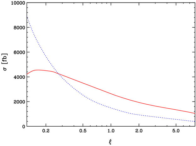
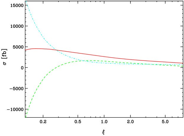
Figure 2: Scale dependence of the total cross section for $pp\rightarrow t\bar{t}b\bar{b}+X$ at the LHC with $\mu_{R}=\mu_{F}=\xi m_{t}$. On the upper panel, the blue dashed curve corresponds to the leading order, whereas the red solid one to the next-to-leading order result. The lower panel shows the scale dependence of the next-to-leading order cross section (red solid curve) decomposed into the contribution of the virtual corrections (green dashed curved) and real radiation (cyan dash-dotted curve).

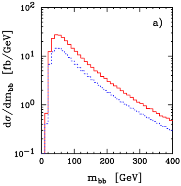
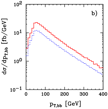
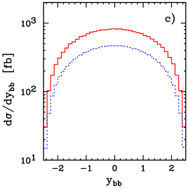
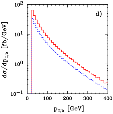
Figure 3: Distribution of the invariant mass $m_{b\bar{b}}$ of the bottom-anti-bottom pair (a), distribution in the transverse momentum $p_{T_{b\bar{b}}}$ of the bottom-anti-bottom pair (b), distribution in the rapidity $y_{b\bar{b}}$ of the bottom-anti-bottom pair (c) and distribution in the transverse momentum $p_{T_{b}}$ of the bottom quark (d) for $pp\rightarrow t\bar{t}b\bar{b}+X$ at the LHC at LO (blue dashed line) and NLO (red solid line). All distributions have been obtained with $\alpha_{max}=0.01$.

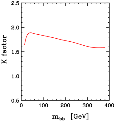
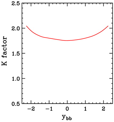
Figure 4: The ratio of the NLO and LO distributions for $pp\rightarrow t\bar{t}b\bar{b}+X$ at the LHC for the invariant mass $m_{b\bar{b}}$ (left panel) and the rapidity $y_{b\bar{b}}$ (right panel) of the bottom-anti-bottom pair.

Subsequently, we turn our attention to the scale dependence, which is given in Tab. 2 for the total cross section for $pp\rightarrow t\bar{t}b\bar{b}+X$ at the LHC at LO and NLO with $\mu_{\footnotesize{\mbox{R}}}=\mu_{\footnotesize{\mbox{F}}}=\xi m_{t}$ for a few distinct values of $\xi$. As expected, we observe a reduction of the scale uncertainty while going from LO to NLO. Varying the scale up and down by a factor 2 changes the cross section by +70% and -38% in the LO case, while in the NLO case we have obtained a variation of the order +33% and -27%. Our findings can be summarized as follows

$$\sigma^{\mbox{\footnotesize{LO}}}_{t\bar{t}b\bar{b}}(\mbox{LHC},m_{t}=\mbox{176.2 GeV},\mbox{CTEQ6L1})={1489.2~{}}^{\footnotesize{\mbox{+1036.8 (70\%)}}}_{-\footnotesize{\mbox{~{}~{}565.8 (38\%)}}}~{}~{}\mbox{fb}\;,$$ (25)

$$\sigma^{\mbox{\footnotesize{NLO}}}_{t\bar{t}b\bar{b}}(\mbox{LHC},m_{t}=\mbox{176.2 GeV},\mbox{CTEQ6M})={2636~{}}^{\footnotesize{\mbox{+862 (33\%)}}}_{-\footnotesize{\mbox{703 (27\%)}}}~{}~{}\mbox{fb}\;.$$ (26)

As can been easily seen from Tab. 2, choosing a scale too small (too large) will correspond to a very large negative (positive) correction. Unfortunately, this large scale variation and the size of the corrections themselves, imply that if a meaningful analysis were required in the present setup, a full NNLO study would be indispensable. As the latter will remain out of reach in the nearest future, it seems that, as already suggested in [24], additional cuts must be introduced in order to reduce the NLO corrections. Only then will this process, which constitutes the main irreducible background, not put in danger the feasibility of Higgs boson searches in the $t\bar{t}H$ channel.

In Fig. 2 we show the result for the scale dependence graphically. Since we confirm the findings of [23, 24] for all other numbers, we will not present the scale dependence with the renormalization and factorization scales varied independently, which can be found in that work. On the other hand it is entertaining to see the final scale dependence for both scales equal emerge out of the two contributions (virtual and real), as also depicted in Fig. 2. Of course, the separation is entirely unphysical, but well defined once we state that we use what is now called the ‘t Hooft-Veltman [79] version of the dimensional regularization, with the integrals as defined in [30]. The large cancellation for small scale values is the source of the rising integration errors quoted in Tab. 2.

The entirely new result, which has not been presented in the literature until now, are the differential distributions for the four simplest observables, namely the invariant mass, transverse momentum and rapidity of the two-$b$-jet system, as well as the transverse momentum of the single $b$-jet. These results can be found in Fig. 3 and have been obtained with $\alpha_{max}=0.01$. The histograms for $\alpha_{max}=1$ are of similar quality, but we have refrained from averaging over the two statistically independent evaluations. Clearly, the distributions show the same large corrections, which turn out to be relatively constant contrary to the case of quark initial states as shown in [23].

The histograms can also be turned into dynamical K-factors, which we show in two cases in Fig. 4, namely for the invariant mass $m_{b\bar{b}}$ and the rapidity $y_{b\bar{b}}$ of the two-$b$-jet system. For those two cases, they are simply defined as

$$K(m_{b\bar{b}})=\frac{d\sigma^{NLO}/dm_{b\bar{b}}}{d\sigma^{LO}/dm_{b\bar{b}}}\;,$$ (27)

and

$$K(y_{b\bar{b}})=\frac{d\sigma^{NLO}/dy_{b\bar{b}}}{d\sigma^{LO}/dy_{b\bar{b}}}\;,$$ (28)

respectively. As already anticipated above, we notice that they have a relatively small variation, when compared with their size.

4 Conclusions

We have presented a complete study of the $pp\rightarrow t\bar{t}b\bar{b}+X$ process at the LHC at the next-to leading order in QCD. Our results agree with the previous study of [23, 24], for all the numbers given in that work. This fact alone constitutes a powerful proof that our fully automatic system can be applied in analyses of realistic processes for the Large Hadron Collider (and for any other collider for that matter).

One conclusion, which follows from the large observed corrections, is that in view of the importance of the process under study as background for Higgs boson production in association with a top quark pair, a more detailed phenomenological analysis is necessary. We postpone such work for the future.

As a completely technical detail, our work provides the last missing formulae for the dipole subtraction formalism with a dependence on a dipole phase space restriction parameter. This allowed for internal tests, as well as useful speed-ups of the calculation.

Appendix A Integrated dipoles with emitter and spectator in the final state

In this Appendix, we give the formulae necessary for a complete implementation of the phase space restriction in the dipole subtraction formalism. We follow closely the notation of [55], and present only the minimum necessary for an implementation in a numerical program.

As stated before, the only missing ingredient concerns the case with a final state emitter and final state spectator. The relevant kinematical variable is

$$y_{ij,k}=\frac{p_{i}p_{j}}{p_{i}p_{j}+p_{i}p_{k}+p_{j}p_{k}}\;,$$ (29)

where $p_{i},p_{j}$ are the momenta of the emitter pair and $p_{k}$ is the momentum of the spectator. We consider the case, where $m_{i}^{2}=p_{i}^{2}=0$, and thus ignore the splitting of a gluon into a pair of massive quarks. Note that the splitting of a heavy quark into a heavy quark and a gluon in the presence of a massless spectator, as well as the splitting of a massless quark in the presence of a massive spectator have already been covered in [63]. The remaining options can be found below.

The upper limit on $y_{ij,k}$ without a phase space restriction is

$$y_{+}=1-\frac{2\mu_{k}(1-\mu_{k})}{1-\mu_{j}^{2}-\mu_{k}^{2}}\;,$$ (30)

where $\mu_{j,k}=m_{j,k}/\sqrt{Q^{2}}$, with $Q=p_{i}+p_{j}+p_{k}$. The restriction is imposed by adding the following condition

$$y_{ij,k}<\alpha\;.$$ (31)

Clearly, we will only observe a modification if

$$\alpha<y_{+}\;.$$ (32)

In such a case, we write the integrated dipole function corresponding to Eq. 5.22 of [55] as

$$I_{ij,k}(\epsilon)\rightarrow I_{ij,k}(\epsilon,\alpha)=I_{ij,k}(\epsilon)+\Delta I_{ij,k}(\alpha)\;.$$ (33)

Notice that, since setting a minimum value of $y_{ij,k}$ screens from all divergences, the additional term $\Delta I_{ij,k}(\alpha)$ is finite and can be obtained by integration over the four-dimensional phase space, thus simplifying substantially the calculation. Indeed, we will use the phase space of Eq. 5.11 from [55], with $\epsilon=0$ and the following insertion

$$\int[\mbox{d}p_{i}(\tilde{p}_{ij},\tilde{p}_{k})]\rightarrow\int[\mbox{d}p_{i}(\tilde{p}_{ij},\tilde{p}_{k})]\theta(y_{ij,k}>\alpha)\;.$$ (34)

We first give the result for the eikonal integral defined as

$$\frac{\alpha_{s}}{2\pi}\frac{1}{\Gamma(1-\epsilon)}\left(\frac{4\pi\mu^{2}}{Q^{2}}\right)^{\epsilon}\Delta I^{\mbox{eik}}=\int[\mbox{d}p_{i}(\tilde{p}_{ij},\tilde{p}_{k})]\theta(y_{ij,k}>\alpha)\frac{1}{2p_{i}p_{j}}\frac{8\pi\mu^{2\epsilon}\alpha_{s}}{1-\tilde{z}_{j}(1-y_{ij,k})}\;,$$ (35)

with $\tilde{z}_{j}=p_{j}p_{k}/(p_{i}p_{k}+p_{j}p_{k})$. It can most conveniently be obtained by a variable change, and we therefore parametrize the formulae with

$$x=y_{+}-\alpha+\sqrt{(y_{+}-\alpha)\left(\frac{1}{y_{+}}-\alpha+\frac{4\mu_{j}^{2}\mu_{k}^{2}}{(\mu_{j}^{2}-(1-\mu_{k})^{2})(1-\mu_{j}^{2}-\mu_{k}^{2})}\right)}\;.$$ (36)

We did not attempt to minimize the number of dilogarithms and our result contains sixteen of them

$$\Delta I^{\mbox{eik}}=\frac{1}{v_{jk}} \!\!\!\!\!\left(-\mbox{Li}_{2}\left(\frac{a+x}{a+x_{+}}\right)+\mbox{Li}_{2}\left(\frac{a}{a+x_{+}}\right)+\mbox{Li}_{2}\left(\frac{x_{+}-x}{x_{+}-b}\right)-\mbox{Li}_{2}\left(\frac{x_{+}}{x_{+}-b}\right)\right.$$ (37)

$$+\mbox{Li}_{2}\left(\frac{c+x}{c+x_{+}}\right)-\mbox{Li}_{2}\left(\frac{c}{c+x_{+}}\right)+\mbox{Li}_{2}\left(\frac{x_{-}-x}{x_{-}+a}\right)-\mbox{Li}_{2}\left(\frac{x_{-}}{x_{-}+a}\right)$$

$$-\mbox{Li}_{2}\left(\frac{b-x}{b-x_{-}}\right)+\mbox{Li}_{2}\left(\frac{b}{b-x_{-}}\right)-\mbox{Li}_{2}\left(\frac{x_{-}-x}{x_{-}+c}\right)+\mbox{Li}_{2}\left(\frac{x_{-}}{x_{-}+c}\right)$$

$$+\mbox{Li}_{2}\left(\frac{b-x}{b+a}\right)-\mbox{Li}_{2}\left(\frac{b}{b+a}\right)-\mbox{Li}_{2}\left(\frac{c+x}{c-a}\right)+\mbox{Li}_{2}\left(\frac{c}{c-a}\right)$$

$$+\log\left(c+x\right)\log\left(\frac{(a-c)(x_{+}-x)}{(a+x)(c+x_{+})}\right)-\log(c)\log\left(\frac{(a-c)x_{+}}{a(c+x_{+})}\right)$$

$$+\log\left(b-x\right)\log\left(\frac{(a+x)(x_{-}-b)}{(a+b)(x_{-}-x)}\right)-\log(b)\log\left(\frac{a(x_{-}-b)}{(a+b)x_{-}}\right)$$

$$-\log\left((a+x)(b-x_{+})\right)\log\left(x_{+}-x\right)+\log\left(a(b-x_{+})\right)\log(x_{+})$$

$$+\log(d)\log\left(\frac{(a+x)x_{+}x_{-}}{a(x_{+}-x)(x_{-}-x)}\right)+\log\left(\frac{x_{-}-x}{x_{-}}\right)\log\left(\frac{c+x_{-}}{a+x_{-}}\right)$$

$$\left.+\frac{1}{2}\log\left(\frac{a+x}{a}\right)\log\left(a(a+x)(a+x_{+})^{2}\right)\right)\;,$$

where

$$a = \frac{2\mu_{k}}{1-\mu_{j}^{2}-\mu_{k}^{2}}\;,$$ (38)

$$b = \frac{2(1-\mu_{k})}{1-\mu_{j}^{2}-\mu_{k}^{2}}\;,$$ (39)

$$c = \frac{2\mu_{k}(1-\mu_{k})}{1-\mu_{j}^{2}-\mu_{k}^{2}}\;,$$ (40)

$$d = \frac{1}{2}(1-\mu_{j}^{2}-\mu_{k}^{2})\;,$$ (41)

and

$$x_{\pm} = \frac{(1-\mu_{k})^{2}-\mu_{j}^{2}\pm\sqrt{\lambda(1,\mu_{j}^{2},\mu_{k}^{2})}}{1-\mu_{j}^{2}-\mu_{k}^{2}}\;,$$ (42)

$$v_{jk} = \frac{\sqrt{\lambda(1,\mu_{j}^{2},\mu_{k}^{2})}}{1-\mu_{j}^{2}-\mu_{k}^{2}}\;,$$ (43)

with $\lambda$ the Källen function

$$\lambda(x,y,z)=x^{2}+y^{2}+z^{2}-2xy-2xz-2yz\;.$$ (44)

Besides the eikonal integral we will also need the collinear integrals (for this and future works with massive quarks), which are implicitly defined as (in complete analogy to Eqs. 5.23-5.25 of [55])

$$\Delta I_{gQ,k} = C_{F}\left[2\Delta I^{\mbox{eik}}+\Delta I^{\mbox{coll}}_{gQ,k}\right]\;,$$ (45)

$$\Delta I_{q\bar{q},k} = T_{R}\Delta I^{\mbox{coll}}_{q\bar{q},k}\;,$$ (46)

$$\Delta I_{gg,k} = 2C_{A}\left[2\Delta I^{\mbox{eik}}+\Delta I^{\mbox{coll}}_{gg,k}\right]\;.$$ (47)

The respective results read ($\mu_{j}$ refers to the mass of the heavy quark)

$$\Delta I_{gQ,k} = \left(\frac{3}{2}(1+\alpha)+\frac{1}{1-\mu_{k}}-\frac{2(2-2\mu_{j}^{2}-\mu_{k})}{1-\mu_{j}^{2}-\mu_{k}^{2}}+\frac{(1-\alpha)\mu_{j}^{2}}{2(\mu_{j}^{2}+\alpha(1-\mu_{j}^{2}-\mu_{k}^{2}))}\right.$$

$$\left.-2\log\left(\frac{\alpha(1-\mu_{j}^{2}-\mu_{k}^{2})}{(1-\mu_{k})^{2}-\mu_{j}^{2}}\right)+\frac{1+\mu_{j}^{2}-\mu_{k}^{2}}{2(1-\mu_{j}^{2}-\mu_{k}^{2})}\log\left(\frac{\mu_{j}^{2}+\alpha(1-\mu_{j}^{2}-\mu_{k}^{2})}{(1-\mu_{k})^{2}}\right)\right)\;,$$

$$\Delta I_{q\bar{q},k} = \frac{2}{3}\left(\frac{1-\mu_{k}-\alpha(1+\mu_{k})}{1+\mu_{k}}+\log\left(\frac{\alpha(1+\mu_{k})}{1-\mu_{k}}\right)\right)$$

$$+\left(\kappa-\frac{2}{3}\right)\frac{2\mu_{k}^{2}}{1-\mu_{k}^{2}}\log\left(\frac{(1-\alpha)(1+\mu_{k})}{2\mu_{k}}\right)\;,$$

$$\Delta I_{gg,k} = -\frac{11}{6}\left(\frac{1-\mu_{k}-\alpha(1+\mu_{k})}{1+\mu_{k}}+\log\left(\frac{\alpha(1+\mu_{k})}{1-\mu_{k}}\right)\right)$$

$$-\left(\kappa-\frac{2}{3}\right)\frac{\mu_{k}^{2}}{1-\mu_{k}^{2}}\log\left(\frac{(1-\alpha)(1+\mu_{k})}{2\mu_{k}}\right)\;.$$

References

- [1] M. Czakon and A. Mitov, arXiv:0811.4119 [hep-ph].
- [2] K. Melnikov and M. Schulze, JHEP 0908 (2009) 049.
- [3] M. Czakon, A. Mitov and S. Moch, Phys. Lett. B651 (2007) 147.
- [4] M. Czakon, A. Mitov and S. Moch, Nucl. Phys. B798 (2008) 210.
- [5] J. G. Korner, Z. Merebashvili and M. Rogal, Phys. Rev. D77 (2008) 094011.
- [6] M. Czakon, Phys. Lett. B664 (2008) 307.
- [7] R. Bonciani, A. Ferroglia, T. Gehrmann, D. Maitre and C. Studerus, JHEP 0807 (2008) 129.
- [8] C. Anastasiou and S. M. Aybat, Phys. Rev. D78 (2008) 114006.
- [9] B. Kniehl, Z. Merebashvili, J. G. Korner and M. Rogal, Phys. Rev. D78 (2008) 094013.
- [10] R. Bonciani, A. Ferroglia, T. Gehrmann and C. Studerus, JHEP 0908 (2009) 067.
- [11] M. Czakon and A. Mitov, arXiv:0812.0353 [hep-ph].
- [12] M. Beneke, P. Falgari and C. Schwinn, arXiv:0907.1443 [hep-ph].
- [13] M. Czakon, A. Mitov and G. Sterman, arXiv:0907.1790 [hep-ph].
- [14] W. Beenakker et. al., Phys. Rev. Lett. 87 (2001) 201805.
- [15] L. Reina and S. Dawson, Phys. Rev. Lett. 87 (2001) 201804.
- [16] L. Reina, S. Dawson and D. Wackeroth, Phys. Rev. D65 (2002) 053017.
- [17] W. Beenakker et. al., Nucl. Phys. B653 (2003) 151.
- [18] S. Dawson, L. H. Orr, L. Reina and D. Wackeroth, Phys. Rev. D67 (2003) 071503.
- [19] S. Dawson, C. Jackson, L. H. Orr, L. Reina and D. Wackeroth, Phys. Rev. D68 (2003) 034022.
- [20] S. Dittmaier, P. Uwer and S. Weinzierl, Phys. Rev. Lett. 98 (2007) 262002.
- [21] S. Dittmaier, P. Uwer and S. Weinzierl, Eur. Phys. J. C59 (2009) 625.
- [22] A. Lazopoulos, T. McElmurry, K. Melnikov and F. Petriello, Phys. Lett. B666 (2008) 62.
- [23] A. Bredenstein, A. Denner, S. Dittmaier and S. Pozzorini, JHEP 0808 (2008) 108.
- [24] A. Bredenstein, A. Denner, S. Dittmaier and S. Pozzorini, Phys. Rev. Lett. 103 (2009) 012002.
- [25] D. Peng-Fei et. al., arXiv:0907.1324 [hep-ph].
- [26] M. Cammin, J. Schumacher, ATL-PHYS-2003-024.
- [27] A. Kanaki and C. G. Papadopoulos, Comput. Phys. Commun. 132 (2000) 306.
- [28] A. Kanaki and C. G. Papadopoulos, hep-ph/0012004.
- [29] A. Cafarella, C. G. Papadopoulos and M. Worek, Comput. Phys. Commun. 180 (2009) 1941.
- [30] A. van Hameren, C. G. Papadopoulos and R. Pittau, arXiv:0903.4665 [hep-ph].
- [31] G. Ossola, C. G. Papadopoulos and R. Pittau, Nucl. Phys. B763 (2007) 147.
- [32] G. Ossola, C. G. Papadopoulos and R. Pittau, JHEP 0803 (2008) 042.
- [33] M. Czakon, C. G. Papadopoulos and M. Worek, JHEP 0908 (2009) 085.
- [34] P. Draggiotis, M. V. Garzelli, C. G. Papadopoulos and R. Pittau, JHEP 0904 (2009) 072.
- [35] Z. Bern, L. J. Dixon, D. C. Dunbar and D. A. Kosower, Nucl. Phys. B425 (1994) 217.
- [36] Z. Bern, L. J. Dixon, D. C. Dunbar and D. A. Kosower, Nucl. Phys. B435 (1995) 59.
- [37] E. Witten, Commun. Math. Phys. 252 (2004) 189.
- [38] R. Britto, F. Cachazo and B. Feng, Nucl. Phys. B725 (2005) 275.
- [39] A. Brandhuber, S. McNamara, B. J. Spence and G. Travaglini, JHEP 0510 (2005) 011.
- [40] R. Britto, B. Feng and P. Mastrolia, Phys. Rev. D73 (2006) 105004.
- [41] Z. Bern, L. J. Dixon and D. A. Kosower, Annals Phys. 322 (2007) 1587.
- [42] R. K. Ellis, K. Melnikov and G. Zanderighi, JHEP 0904 (2009) 077.
- [43] C. F. Berger et al., Phys. Rev. Lett. 102 (2009) 222001.
- [44] C. F. Berger et. al., arXiv:0907.1984 [hep-ph].
- [45] S. Dittmaier, S. Kallweit and P. Uwer, Phys. Rev. Lett. 100 (2008) 062003.
- [46] J. M. Campbell, R. Keith Ellis and G. Zanderighi, JHEP 0712 (2007) 056.
- [47] V. Hankele and D. Zeppenfeld, Phys. Lett. B661 (2008) 103.
- [48] F. Campanario, V. Hankele, C. Oleari, S. Prestel and D. Zeppenfeld, Phys. Rev. D78 (2008) 094012.
- [49] F. Febres Cordero, L. Reina and D. Wackeroth, Phys. Rev. D78 (2008) 074014.
- [50] J. M. Campbell, R. K. Ellis, F. Febres Cordero, F. Maltoni, L. Reina, D. Wackeroth and S. Willenbrock, Phys. Rev. D79 (2009) 034023.
- [51] F. F. Cordero, L. Reina and D. Wackeroth, Phys. Rev. D80 (2009) 034015.
- [52] B. Jager, C. Oleari and D. Zeppenfeld, Phys. Rev. D80 (2009) 034022.
- [53] NLO Multileg Working Group Collaboration, Z. Bern et. al., arXiv:0803.0494 [hep-ph].
- [54] S. Catani and M. H. Seymour, Nucl. Phys. B485 (1997) 291.
- [55] S. Catani, S. Dittmaier, M. H. Seymour and Z. Trocsanyi, Nucl. Phys. B627 (2002) 189.
- [56] T. Gleisberg and F. Krauss, Eur. Phys. J. C53 (2008) 501.
- [57] M. H. Seymour and C. Tevlin, arXiv:0803.2231 [hep-ph].
- [58] K. Hasegawa, S. Moch and P. Uwer, Nucl. Phys. Proc. Suppl. 183 (2008) 268.
- [59] R. Frederix, T. Gehrmann and N. Greiner, JHEP 0809 (2008) 122.
- [60] Z. Nagy and Z. Trocsanyi, Phys. Rev. D59 (1999) 014020.
- [61] Z. Nagy, Phys. Rev. D68 (2003) 094002.
- [62] J. M. Campbell, R. K. Ellis and F. Tramontano, Phys. Rev. D70 (2004) 094012.
- [63] J. M. Campbell and F. Tramontano, Nucl. Phys. B726 (2005) 109.
- [64] F. Maltoni, K. Paul, T. Stelzer and S. Willenbrock, Phys. Rev. D67 (2003) 014026.
- [65] M. L. Mangano, M. Moretti, F. Piccinini, R. Pittau and A. D. Polosa, JHEP 0307 (2003) 001.
- [66] C. G. Papadopoulos and M. Worek, Eur. Phys. J. C50 (2007) 843.
- [67] P. Draggiotis, R. H. P. Kleiss and C. G. Papadopoulos, Phys. Lett. B439 (1998) 157.
- [68] P. D. Draggiotis, R. H. P. Kleiss and C. G. Papadopoulos, Eur. Phys. J. C24 (2002) 447.
- [69] A. Lazopoulos, K. Melnikov and F. Petriello, Phys. Rev. D76 (2007) 014001.
- [70] T. Binoth, G. Ossola, C. G. Papadopoulos and R. Pittau, JHEP 0806 (2008) 082.
- [71] J. Alwall et. al., Comput. Phys. Commun. 176 (2007) 300.
- [72] C. G. Papadopoulos, Comput. Phys. Commun. 137 (2001) 247.
- [73] R. Kleiss and R. Pittau, Comput. Phys. Commun. 83 (1994) 141.
- [74] S. Catani, Y. L. Dokshitzer and B. R. Webber, Phys. Lett. B285 (1992) 291.
- [75] S. Catani, Y. L. Dokshitzer, M. H. Seymour and B. R. Webber, Nucl. Phys. B406 (1993) 187.
- [76] S. D. Ellis and D. E. Soper, Phys. Rev. D48 (1993) 3160.
- [77] J. Pumplin et. al., JHEP 0207 (2002) 012.
- [78] D. Stump et. al., JHEP 0310 (2003) 046.
- [79] G. ’t Hooft and M. J. G. Veltman, Nucl. Phys. B44 (1972) 189.