Particle Methods For Stochastic Optimal Control Problems
Abstract
When dealing with numerical solution of stochastic optimal control problems, stochastic dynamic programming is the natural framework. In order to try to overcome the so-called curse of dimensionality, the stochastic programming school promoted another approach based on scenario trees which can be seen as the combination of Monte Carlo sampling ideas on the one hand, and of a heuristic technique to handle causality (or nonanticipativeness) constraints on the other hand.
However, if one considers that the solution of a stochastic optimal control problem is a feedback law which relates control to state variables, the numerical resolution of the optimization problem over a scenario tree should be completed by a feedback synthesis stage in which, at each time step of the scenario tree, control values at nodes are plotted against corresponding state values to provide a first discrete shape of this feedback law from which a continuous function can be finally inferred. From this point of view, the scenario tree approach faces an important difficulty: at the first time stages (close to the tree root), there are a few nodes (or Monte-Carlo particles), and therefore a relatively scarce amount of information to guess a feedback law, but this information is generally of a good quality (that is, viewed as a set of control value estimates for some particular state values, it has a small variance because the future of those nodes is rich enough); on the contrary, at the final time stages (near the tree leaves), the number of nodes increases but the variance gets large because the future of each node gets poor (and sometimes even deterministic).
After this dilemma has been confirmed by numerical experiments, we have tried to derive new variational approaches. First of all, two different formulations of the essential constraint of nonanticipativeness are considered: one is called algebraic and the other one is called functional. Next, in both settings, we obtain optimality conditions for the corresponding optimal control problem. For the numerical resolution of those optimality conditions, an adaptive mesh discretization method is used in the state space in order to provide information for feedback synthesis. This mesh is naturally derived from a bunch of sample noise trajectories which need not to be put into the form of a tree prior to numerical resolution. In particular, an important consequence of this discrepancy with the scenario tree approach is that the same number of nodes (or points) are available from the beginning to the end of the time horizon. And this will be obtained without sacrifying the quality of the results (that is, the variance of the estimates). Results of experiments with a hydro-electric dam production management problem will be presented and will demonstrate the claimed improvements.
keywords:
stochastic programming; measurability constraints; discretizationAMS:
90C15, 49M25, 62L20Introduction
Taking into account uncertainties in the decision process has become an important issue for all industries. Facing the market volatilities, the weather whims and the changing policies and regulatory constraints, decision makers have to find an optimal way to introduce their decision process into this uncertain framework. One way to take uncertainties into account is to use the stochastic optimization framework. In this approach, the decision maker makes his decision by optimizing a mean value with regard to the multiple possible scenarios weighted with a probability law.
Stochastic optimization problems often involve information constraints: the decision maker makes his decision after getting observations about the possible scenarios. In the literature, two different communities have dealt with this information issue using different modelling techniques, and therefore different solution methods. The question is: knowing that stochastic optimization problems are often infinite dimensional problems, how can we implement tractable solution methods (which can be implemented using a computer)? To answer this question each community brought its own answers.
The stochastic programming community models the information structure by scenarios trees: this involves Monte Carlo sampling plus some manipulations of the sample trajectories to enforce the tree structure. Then, tractable solution methods for stochastic optimization problems consist in solving deterministic problems over the decision trees. We refer to [16, 12, 10] for further details on these methods. Nevertheless, stochastic programming faces an important difficulty: due to the tree structure, one has a few discretization points (nodes of the tree) at the early stages, which could represent a serious handicap when attempting to synthesizing a feedback law. On the contrary, when approaching the last stages, one has a large number of discretization points but with a future which may be almost or completely deterministic.
The stochastic optimal control community uses special structures of the stochastic optimization problems (time sequentiality and state notions) to model the information constraints through a functional interpretation that leads to the Dynamic Programming Principle. We refer to [4, 5, 6] for further details on this method. However, stochastic dynamic programming is also confronted with a serious obstacle known as the “curse of dimensionality”. In fact, this method leads one to blindly discretize the whole state space without taking into account a, generally nonuniform, state distribution at the optimal solution.
This paper tries to bridge the gap between those two communities. We propose a tractable solution method for stochastic optimal control problems which makes use of the good ideas of both Monte Carlo sampling and variational methods on the one hand, functional handling of the information structure on the other hand. Other related works [8, 20] are still closer to the stochastic programming point of view. In our approach, the same number of discretization (sample) points are used from the beginning to the end of the time horizon, and this discretization grid is adaptive: when transposed into the state space, it reflects the optimal state distribution at each time stage.
The proposed method is of a variational nature in that it is based on gradient calculations which involve the forward state variable integration and the backward adjoint state (co-state) evaluation as in the Pontryagin minimum principle. The purpose is to solve the Kuhn-Tucker necessary optimality conditions of the considered problem (including the information constraints).
This paper is organized as follows. In §1, we discuss how to model the information structure in stochastic optimization problems. Then we derive optimality conditions for stochastic optimization problems with information constraints. In §2, these optimality conditions are specialized to the situation of stochastic optimal control problems. A special attention is paid to the so-called Markovian case in §2.4. The numerical implementation of a resolution method based on Monte Carlo and functional approximations is presented in §3. Finally, in §4, a case study, namely a hydro-electric dam management problem, illustrates the proposed method, and compares it to the standard scenario tree approach.
1 Preliminaries
In this section, we present the main framework of this paper: how to model stochastic optimization problems and how to represent the information structure of such problems. This preliminary section is directly inspired from the works of the System and Optimization Working Group111SOWG, École Nationale des Ponts et Chaussées: Laetitia Andrieu, Kengy Barty, Pierre Carpentier, Jean-Philippe Chancelier, Guy Cohen, Anes Dallagi, Michel De Lara, Pierre Girardeau, Babakar Seck, Cyrille Strugarek. [2, 19, 9].
In the sequel of the paper, the random variables, defined over a probability space , will be denoted using bold letters (e.g. ) whereas their realizations will be denoted using normal letters (e.g. ).
1.1 Modelling information
When unknown factors affect a process that we try to control, we consider a set of possible states of nature among which the true state is supposed to be. Roughly speaking, an information structure is a partition of into a collection of subsets . A posteriori observations will help us to determine in which particular subset of this partition the true state lies. Two extreme cases may be mentioned.
-
1.
If the partition is simply the crude partition , then the a posteriori observations are useless. We will refer to this situation as an open-loop information structure.
-
2.
If the partition is the finest possible one, namely all subsets are singletons, then the a posteriori observations will tell us exactly what is the true state of nature . This is the situation of perfect knowledge prior to making our decisions.
In between, after the a posteriori observations become available, we will remain with some uncertainty about the true , that is we will know in which particular the true state lies but all ’s in that are still possible. Moreover, in dynamic situations, new observations may become available at each time stage and a partition of corresponding to this information structure must be considered at each time stage. We refer to the general case as a closed-loop decision process.
In order to have a framework in which various operations on information structures become possible, probability theory introduces so-called -algebras or -fields, random variables and a pre-order relation between random variables. The latter is called measurability.222A random variable is measurable with respect to another random variable if and only if the -field generated by the first is included into the one generated by the second: . In this paper, we will not give further details on these definitions. Instead, we refer the reader to [7] for further details on the probability and measurability theory.
We refer the reader to [17] for further details on information structure and probability theory. As far as this paper is concerned, we here state a result found in [17, Theorem 8 p.108] giving the main properties of the measurability relation between random variables.
Proposition 1 (Measurability relation).
Let be a probability space, let and be two random variables taking their values in and respectively. The following statements are equivalent:
-
1.
,
-
2.
,
-
3.
, a measurable mapping such that ,
-
4.
.
1.2 Modelling a stochastic optimization problem
In this section, we consider two interpretations of a stochastic optimization problem: an algebraic one in which the information constraint is modelled through the standard measurability relation (Statement of Proposition 1), and a functional interpretation in which we use the functional equivalent of measurability relation (Statement of Proposition 1).
1.2.1 Algebraic interpretation
Let be a probability space and let be a random variable taking values in (noise space). We denote by the control space and by the functional space . The cost function is defined as the expectation of a normal integrand333See [18, Definition 14.27]. We remind that the normal integrand assumption is done to ensure measurability properties [18, Proposition 14.28].
The feasible set accounts for two different constraints:
-
•
almost sure constraints:
(1) where is a measurable set-valued mapping (see [18, Definition 14.1]) which is convex and closed valued, and
-
•
measurability constraints:
(2) where is a given sub--field of .
From their respective definitions, it is easy to prove that is a closed subspace of (indeed ) and that is a closed convex subset of .
The optimization problem under consideration is to minimize the cost function over the feasible subset . The first model representing the stochastic optimization problem is thus
| (3) |
This interpretation is called algebraic as it uses an algebraic relation (measurability) to define the information structure of Problem (3).
1.2.2 Functional interpretation
According to Proposition 1, a functional model for stochastic optimization problems is available, in which the optimization is achieved with respect to functions called feedbacks. Indeed, let
-
•
be a random variable (called the observation) taking value in ,
-
•
be the space where is the Borel -field of and the image of the probability measure by ,
-
•
be the subset of defined by
We define the cost function as . We are interested in the functional optimization problem:
| (4) |
Proposition 2.
Proof.
This is a straightforward consequence of Proposition 1 and of the definition of the feasible sets in both problems. ∎
1.3 Optimality conditions for a stochastic optimization problem
Previous works dealt with optimality conditions for stochastic optimal control problems [15, 13]. This paragraph can be viewed as a slight extension of [15] when considering a stochastic optimization problem subject to almost-sure and measurability constraints.
We consider Problem (3) presented in §1.2. We recall that the feasible set is the intersection of a closed convex subset and of a linear subspace . In order to apply the results given in Appendix A, we first establish the following lemma.
Lemma 3.
Proof.
We first prove that . Indeed, let . From the definition of almost sure constraints, we have , with . By definition of the projection, is solution of the optimization problem
Using [18, Theorem 14.60] (interchange of minimization and integration), we obtain
| (5) |
hence the claimed property.
The main result of this section is given by the following theorem.
Theorem 4.
Assume that is a -mesurable and closed convex valued mapping, that function is a normal integrand such that is differentiable -a.s. and that for all . Let be a solution of Problem (3). Then
| (6) |
Proof.
The differentiability of is a straightforward consequence of both the integral expression of and the differentiability assumption on . Moreover the expression of the derivative of is given by
Let be a solution of (3). From Lemma 3 and Proposition 13 in the Appendix, we obtain
this last expression being equivalent to (6) thanks to the characterization of the conditional expectation as a projection and the expression of . ∎
Using the equivalent statements (34c), the optimality conditions given by Theorem 6 can be reformulated as
This last formulation can be used in practice to solve Problem (3) using a projected gradient algorithm. The projection over involves random variables, but we saw in the proof of Lemma 3 that can be performed in a pointwise manner ( per ), so that the implementation of the algorithm is effective.
2 Stochastic optimal control problems
Stochastic optimal control problems rest upon the same framework as stochastic optimization problems: they can be modelled as closed-loop stochastic optimization problems with a sequential time structure. In this section, we deal with the algebraic interpretation of stochastic optimal control problems in a discrete time framework. We will derive optimality conditions following the same principle as in §1.3.
2.1 Problem formulation
We consider a stochastic optimal control problem in discrete time, denoting the time horizon. At each stage , we denote by the noise space at time . Let be a set of random variables defined on and taking values in , and let . The noise process of the problem is a random vector such that , with .
At each stage , we denote by the control space and by the space of square integrable random variables taking values in . At , the decision maker makes a decision (a control) . Let . The control process of the problem is a random vector such that , with . We also assume that each control variable is subject to almost-sure constraints. More precisely, for all , let be a set-valued mapping (random set), let and let . The almost-sure constraints writes
| (7) |
2.1.1 Dynamics
At each stage , we denote by the state space at time . Let be a set of random variables defined on and taking values in , and let . The state process of the problem is a random vector such that , with . It arises from the dynamics of the system, namely
| (8a) | ||||
| (8b) | ||||
Remark 2.
The shift on the time index between the random variable and the control on the one hand and the noise on the other hand enlightens the fact that we are in the so-called decision-hazard scheme: at time , the decision maker chooses a control variable before having any information about the noise which affects the dynamics of the system.
2.1.2 Cost function
We consider at each stage , an “integral” cost function . Moreover, at the final stage , we consider a final cost function . Summing up all these instantaneous costs, we obtain the overall cost function of the problem
and the decision maker has to choose the control variables in order to minimize the overall cost expectation
| (9) |
2.1.3 Information structure
Generally speaking, the information available on the system at time is modelled as a random variable , where is the observation space. Let be the set of random variables taking their values in . We suppose that there exists an observation mapping such that . For all , we denote by the sub--field of generated by the random variable :444Note that the -fields ’s are “fixed”, in the sense that they do not depend on the control variable .
The decision maker knows when choosing the appropriate control at time , so that the information constraint is . Using the notations and , the measurability constraints of the problem writes
| (10) |
We also introduce the sequence of -fields associated with the noise process , where is the -field generated by the noises prior to :
This sequence is a filtration as it satisfies the inclusions . When , we are in the case of complete causal information.
2.1.4 Optimization problem
According to the notation given in the previous paragraphs, the stochastic optimal control problem we consider here is
| (11a) | |||
| subject to both the dynamics constraints (8) and the control constraints | |||
| (11b) | |||
We follow here the algebraic interpretation of an optimization problem given in §1.2, as the information structure is defined using a measurability relation.
In the way we modelled Problem (11b), we have to minimize the cost function with respect to both and under the dynamics constraints (8). But the state variables are in fact intermediary variables and it is possible to eliminate them by recursively incorporating the dynamics equations (8) into the cost function (9). The resulting cost function only depends on the control variables . Its expression is , with
In this setting, Problem (11b) is equivalent to
| (12) |
The derivatives of the cost function can be obtained from the derivatives of using the well known adjoint state method. This is based on the following result stated here without proof.
Proposition 5.
Assuming that functions and are continuously differentiable with respect to their first two arguments and that function is continuously differentiable, the partial derivatives of with respect to are given by
where the state vector satisfies the forward dynamics equation
whereas the adjoint state (or co-state) vector is chosen to satisfy the backward dynamics equation
2.1.5 Assumptions
In order to derive optimality conditions for Problem (11b), we make the following assumptions.
Assumption 1 (Constraints structure).
-
are closed convex set-valued mappings, .
Assumption 2 (Differentiability).
-
1.
Functions (dynamics) and (cost) are continuous differentiable with respect to their first two arguments (state and control), .
-
2.
Function (final cost) is continuously differentiable.
-
3.
Functions and are normal integrands, .
-
4.
The derivatives of , and are square integrable, .
Assumption 3 (Nonanticipativity and measurability).
-
1.
.
-
2.
Mappings are -measurable, .
Assumption 2 will allow us all integration and derivation operations needed for obtaining optimality conditions. The measurability condition on in Assumption 3 expresses that the almost-sure constraints must at least have the same measurability as the decision variables. The first condition in Assumption 3 expresses the causality of the problem: the decision maker has no access to information in the future! Under this assumption, there exists a measurable mapping such that the information variable writes
Proposition 6 (Constraints structure).
For all ,
-
1.
is a closed convex subset of ,
-
2.
.
2.2 Optimality conditions in stochastic optimal control problems
We present here necessary optimality conditions for the stochastic optimal control problem (11b), which are an extension of the conditions given in Theorem 6.
2.2.1 Non-adapted optimality conditions
A first set of optimality conditions is given in the next theorem.
Theorem 7.
Proof.
The conditions given by Theorem 13 are called non-adapted optimality conditions because the dual random process is not adapted to the natural filtration , that is, generally depends on the future. We will see in the next section that similar optimality conditions can be written with help of an adapted dual random process.
2.2.2 Adapted optimality conditions
The following theorem presents optimality conditions involving an adapted dual random process.
Theorem 8.
Proof.
All assumptions of Theorem 13 are met, so that there exists a random process satisfying (13). Define for all the random variable by
By construction, the process is adapted to the filtration . At stage , we have
because is -measurable. For all , using the law of total expectation and since all variables , and are -measurable, we deduce from (13) that
hence the adapted backward dynamics equations given in (14).
Note that in the optimality conditions given in Theorem 14, at each stage , the gradient is projected over the subspace generated by the observation -field , whereas the adapted dual random variable is projected over the subspace generated by which corresponds to the natural filtration of Problem (11b).
2.3 Optimality conditions in the Markovian case
As far as information structure is concerned, the optimality conditions (13) and (14) were obtained assuming only nonanticipativeness (see Assumption 3) and the fact that the observation -fields do not depend on the decisions . The last assumption allows us to avoid the so-called “dual effect of control” (see [3] for further details). Another feature often available in practice for the information structure is the “perfect memory” property, which intuitively means that the information is not lost over time. The last property implies that is a filtration, namely
We will assume in the sequel that the perfect memory property holds, and we will moreover assume complete causal noise observation, so that .555Note that complete causal noise observation implies the perfect memory property, as far as is a filtration. Then both optimality conditions (13) and (14) involve conditional expectations with respect to a random observation variable the dimension of which increases with time (a new noise random variable becomes available at each stage ). This leads to a computational difficulty, of the same nature as the so-called curse of dimensionality. To address this difficulty, it would be an easier situation to have a constant dimension for the observation space, as in the stochastic dynamic programming principle [5, 6] when the optimal control at only depends on the state variable at the same time stage. We thus consider new (more restrictive) assumptions which match the stochastic optimal control framework an lead us to the desired situation.
Assumption 4 (Markovian case).
-
1.
(perfect memory and causal noise observation).
-
2.
The random variables are independent (white noise).
-
3.
The mappings are constant (deterministic constraints):
.
The standard formulation of a stochastic optimal control problem in the Markovian case is to assume that the state is completely and perfectly observed. The problem formulation is accordingly
| (15a) | |||
| subject to both the dynamics constraints (8) and the control constraints | |||
| (15b) | |||
We now consider the optimality conditions (13) and (14) and we specialize them to the Markovian case.
2.3.1 Markovian case: non-adapted optimality conditions
We present a non-adapted version of the optimality conditions of Problem (11b) with Markovian assumptions. We begin by presenting a result inspired by the stochastic dynamic programming principle.
Theorem 9.
Proof.
First, Assumption 3 being implied by Assumption 4, the existence of the process satisfying (13) is given by Theorem 13. Denoting by the Hamiltonian at time , namely , optimality conditions (13d) and (13e) write
| (16a) | |||
| (16b) | |||
The proof of statements and is obtained by induction. For the sake of simplicity, we first prove the result when , so that (16b) reduces to the equality condition:
| (16c) |
-
•
At stage , we know from (13c) that , with being a measurable function,666In fact, . From Assumption 2, is a continuous mapping. and hence
(17a) Then using (13b), the optimality condition (16c) takes the form: and being both -measurable random variables, and being independent of (white noise assumption), we deduce that the conditional expectation in the last expression reduces to an expectation. Let denotes the function resulting from its integration, namely is a mesurable mapping,777in fact a continuous one (from Assumption 2) and the optimality condition writes Using the measurable selection theorem available for implicit measurable functions [14, Theorem 8],888See for instance [21, Section 7] for a survey of measurable selection theorems corresponding to the implicit case. Note that [14, Theorem 8] needs a particular assumption concerning the -field equipping . We assume here that such assumption holds. we deduce that there exists a measurable mapping such that . As a conclusion, the control variable satisfies the optimality condition (16c) at and is such that (17b) -
•
At stage , assume that . Then there exists a measurable function such that
(18a) The optimality condition (16c) at stage takes the form With the same reasoning as at stage , we deduce that this conditional expectation reduces to an expectation, so that the optimality condition writes being a measurable function given by Using again [14, Theorem 8], we deduce that there exists a measurable mapping such that satisfies the optimality condition (16c) at . We have accordingly (18b) Ultimately, starting from the optimality condition (16a), namely using the induction assumption (18a) together with (18b) and (13c), we obtain that We conclude that so that the desired result holds true.999Note that we obtained as an intermediate result that .
Let’s go now to the general case . From (34), the optimality condition (16b) is again equivalent to an equality condition:
and the same arguments as in the previous case remain valid.
At last, from , and the white noise assumption, we deduce that depends on only through , so that
Statement is thus satisfied and the proof is complete. ∎
In the Markovian case, the optimal solution of Problem (11b) (measurability with respect to all past noise variables) satisfies the measurability constraints of Problem (15b) (measurability with respect to the current state variable). The two problems are equivalent (same and ). In fact, the feasible set of (11b) contains the feasible set of (15b), and Theorem 9 shows us that any optimal solution of (11b) is feasible for (15b), and is therefore also optimal also for (15b). Ultimately, the optimality conditions of Problem (15b) can be written as
| (19a) | |||
| (19b) | |||
| (19c) | |||
| (19d) | |||
| (19e) | |||
Remark 3.
Let and be the gradient processes associated with (13) and (19) respectively:
Unlike Problem 11b, we are unable to compute the optimality conditions (19) of Problem (15b) by differentiating the Lagrangian function, because the conditioning term depends itself on the control variables . Consequently, is not claimed to represent the projected gradient of Problem (15b). The equality between the gradient and holds true only at the optimum.
2.3.2 Markovian case: adapted optimality conditions
We now present the adapted version of the optimality conditions of Problem (11b) under Markovian assumptions.
Theorem 10.
Proof.
The proof follows the same scheme as the one of Theorem 9. We just point out that and implies that . ∎
From the equivalence between Problem (11b) (measurability with respect to the past noise) and Problem (15b) (measurability with respect to the state) in the Markovian framework, we may consider that the optimality conditions of Problem (15b) in the adapted version are
| (20a) | |||
| (20b) | |||
| (20c) | |||
| (20d) | |||
| (20e) | |||
The optimality conditions (19) and (20) involve conditional expectations with respect to the state variable the dimension of which is, in most cases, fixed, that is, it does not depend on the time stage. In order to solve Problem (11b) (and equivalently Problem (15b)), we have to discretize those conditions and in particular to approximate the conditional expectations. The literature on conditional expectation approximation only offers biased estimators with an integrated squared error depending on the dimension of the conditioning term. On the contrary, approximating an expectation through a Monte-Carlo technique involves non-biased estimators the variance of which does not depend on the dimension of the underlining space. In the next section, we propose a functional interpretation of the stochastic optimal control problem in order to get rid of those conditional expectations and deal only with expectations.
2.4 Optimality conditions from a functional point of view
Consider the stochastic optimal control Problem (11b). Under Markovian assumptions, we have shown in §2.3 that it is equivalent to Problem (15b) and that (20) is a set of necessary optimality conditions. Hereafter we transform the optimality conditions (20) using Theorem 10 and the functional interpretation of the measurability relation between random variables (see Proposition 1).
Theorem 11.
Suppose that Assumptions 1, 2 and 4 are fulfilled, and assume that there exist two random processes and solution of Problem (11b). Let be a random process satisfying the optimality conditions (14). Then there exists two sequences of mappings and , and , such that for all ,
| (21a) | |||
| (21b) | |||
| (21c) | |||
| (21d) | |||
with and the probability measure associated with .
Proof.
By Theorem 10, the random processes and are such that and . By Proposition 1, there exist measurable mappings and such that and . From , we deduce that :
Since , we obtain that .
The co-state dynamic equations in (20) rewrites
which, using , becomes
From the white noise assumption, the random variable is independent of , so that the conditional expectation turns out to be just an expectation with respect to the noise random variable. The co-state dynamics equation writes accordingly as a functional equality:
Using similar arguments, we easily obtain from the last condition in (20):
which completes the proof. ∎
Theorem 11 provides the new functional optimality conditions (21) for Problem (11b) in the Markovian case. These optimality conditions do not involve conditional expectations but just expectations. Therefore, we may hope that, in the approximation process of these conditions, we will obtain non biased estimates the variance of which will not depend on the dimension of the state space.
3 Adaptive discretization technique
In this section we develop tractable numerical methods for obtaining the solution of Problem (11b). We will limit ourselves here to the Markovian framework, but methods for all cases described in §2 can be found in [9]. We briefly discuss two classical solution methods, namely stochastic programming and dynamic programming. Then we present an adaptive mesh algorithm which consists in discretizing the optimality conditions obtained at §2.4 and in using them in a gradient-like algorithm.
3.1 Discrete representation of a function
As far as numerical resolution is concerned, we need to manipulate functions which are infinite dimensional objects and which, in most cases, do not have a closed-form expression. Thus we must have a discrete representation of such an object. Let be a function. We suppose that we have at disposal a fixed or variable grid in , that is a collection of elements in :
A point will be called a particle. In order to obtain a discrete representation of , we define its trace, that is a grid on which corresponds to the values of on :
We denote by the trace operator which, with any function , associates the couple of grids , that is the points . On the other hand, knowing the trace of , we need to compute an approximation of the value taken by at any . Let be an interpolation-regression operator which, with any couple of grids , associates representing the initial function. Such an interpolation-regression operator may be defined in different ways (polynomial interpolation, kernel approximation, closest neighbor, etc).
3.2 Stochastic programming
One way to discretize stochastic optimal control problems of type (11b) is to model the information structure as a decision tree.
-
1.
First, simulate a given number of scenarios of the noise process. Then, by some tree generation procedures (see e.g. [16] or [12]), organize these scenarios in a scenario tree (at any node of any time stage , there is a single past trajectory but multiple futures: see Figure 1).
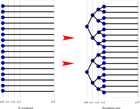
Fig. 1: From scenarios to a tree -
2.
Second, write the components of the problem (state dynamics and cost expectation) on the scenario tree (note that the information constraints are built-in in such a tree structure).
Then the approximation on the scenario tree of Problem (11b) is solved using an appropriate (deterministic) non-linear programming package. The optimal solution consists of state and control particles at each node of the tree. An interpolation-regression procedure (as suggested at §3.1) has to be performed at each time stage in order to synthesize a feedback law.
Such a methodology is relatively easy to implement and need not in fact any Markovian assumption. Nevertheless, it faces a serious drawback: at the first time stages (close to the tree root), only a few particles — or nodes — are available, and experience shows that the estimates of the optimal feedback they provide has a relatively weak variance (because the number of pending scenarios at each such node is still large enough); on the contrary, at the final time stages (near the tree leaves), a large number of particles is available, but with a huge variance. In both cases, the feedback synthesis (the interpolation-regression process from the available grid) will be inaccurate. Such an observation will be highlighted later on the case study §4.
3.3 Stochastic dynamic programming
We consider Problem (11b) in the Markovian case, which is thus equivalent to Problem (15b). From Theorem 9, the optimal control process can be searched as a collection of feedback laws depending on the process state , that is
According to the Dynamic Programming Principle, the resolution is built up backward from to by solving the Bellman equation at each time stage for all state values . Such a principle leads to the following algorithm [5, 6].
Algorithm 1 (Stochastic Dynamic Programming).
-
•
At stage ,
define the Bellman function as -
•
Recursively for ,
compute the Bellman function asthe optimal feedback law being obtained as
This algorithm is only conceptual because it operates on infinite dimensional objects (and expectations cannot always be evaluated analytically). We must indeed manipulate those objects as indicated at §3.1. For every , let be a fixed grid of discretization points in the state space . We approximate the functions appearing in Algorithm 1 by their trace over that grid:
We also need to approximate the expectations by the Monte Carlo method. Let denote independent and identically distributed scenarios of the random noise process. The discretized stochastic dynamic programming algorithm is as follows.
Algorithm 2 (Discretized Stochastic Dynamic Programming).
-
•
At stage ,
compute the trace of the Bellman function : -
•
Recursively for ,
approximate by interpolation-regression:compute the two grids and , that is, for each ,
and obtain the feedback law as
Remark 4.
The interpolation-regression operator is in most cases mandatory in Algorithm 2. As a matter of fact, for a given time stage and a given control value , there usually does not exist any index such that , which means that has to be computed out of the grid . Note however that the Bellman function at time stage is known analytically, so that interpolation is not needed for .
This method faces an important difficulty: the curse of dimensionality. In fact, one generally discretizes each state coordinate at each time stage using a scalar grid and a fixed number of points. Therefore, the grid is obtained as the Cartesian product of the scalar grids over all the coordinates. Thus, the number of particles of that grid increases exponentially with the state space dimension. This is the well-known drawback of most methods derived from Dynamic Programming, which do not take advantage of the repartition of the optimal state particles in the state space in order to concentrate computations in significant parts of the state space.
3.4 The adaptive mesh algorithm
Considering the difficulties faced by both stochastic and dynamic programming methods, we propose an alternative method for solving Problem (11b) in the Markovian case. The method, based on optimality conditions (21), aims at
-
•
dealing with the same number of noise particles from the beginning of the time horizon to the end: we thus hope that the generated feedback law estimators will have a reduced and fixed variance during all time stages;
-
•
attempting to alleviate the curse of dimensionality by operating on an adaptive discretization grid automatically generated from the primary noise discretization grid.
3.4.1 Approximation
Let us denote by a set of independent and identically distributed scenarios obtained from the noise random process. Given random control grids for , we can compute the state random grids by propagating the state dynamics equation:
| (22a) | |||
| (22b) | |||
The feedback at time stage is obtained using an interpolation-regression operator on the grids . Note that the state space grids are not a priori fixed as in Dynamic Programming methods. They are in fact adapted to the control particules, as they change whenever the decision maker changes its control strategy.
Remark 5.
If the optimal state is concentrated in a region of the state space, the optimal feedback will be synthesized only inside that region. In fact we need not compute it elsewhere, because the state will hardly reach other regions.
In order to obtain approximations of the co-state functions introduced at Theorem 11, we compute particles by integrating the co-state backward dynamic equation over the state grids . We thus obtain co-state grids , and make use of interpolation-regression operators in order to compute the co-state function for values out of the current grid. More specifically, the process is initiated with ; then, for all , one computes:
| (23a) | |||
| (23b) | |||
Ultimately, for all and for all , the gradient particles are obtained as
| (24) |
As already noticed, the direction associated with these particles represents the gradient only at the optimum.
3.4.2 Algorithm
We can now derive a descent-like algorithm to solve Problem (11b) under Markovian assumptions. At each iteration, state particles are propagated forward — with no interaction between particles — then, co-state particles are propagated backward — now with interaction caused by the regression-interpolation operations). Then, gradient particles are computed using (24) and the control particles are updated using a gradient-like method. Ultimately, a functional representation of the feedback laws is obtained thanks to a regression-interpolation operator.
Algorithm 3.
-
•
Step .
Let be the initial control grids. -
•
Step .
-
1.
Compute the state grids by propagating the dynamics (22) with .
-
2.
Compute both co-state grids and functional approximations by propagating the dynamics (23) with and .
-
3.
Compute the gradient particles using Equation (24) with , and .
-
4.
For all and , update the control particles by performing a projected gradient step:
-
5.
Stop if some degree of accuracy is reached. Else set and iterate.
-
1.
-
•
Step .
-
1.
Set the grids:
-
2.
Obtain for all the feedback law:
-
1.
The only a priori discretization made during this algorithm is relative to the noise sampling. Once such a discretization has been performed, all other grids used to ultimately obtain the feedback laws are derived by integrating dynamic equations. In addition, no conditional expectation approximations are involved in the process. We just approximate expectations using Monte Carlo techniques, and it is well-known that the variance of such an approximation does not depend on the dimension of the underlying space. The only space-size dependent operations are in fact the interpolation operators used to approximate the co-state mappings during the iterative process, plus the feedback laws once convergence is achieved.
Furthermore, this adaptive discretization makes computations concentrate in effective state space regions, unlike dynamic programming which explores the whole state space.
4 Case study
We consider the production management of an hydro-electric dam. The problem is formulated as a stochastic optimal control, and we consider solving it by the three methods described in §3.
4.1 Model
The problem is formulated in discrete time over hours using a constant time step of one hour. The index (where ) defines the time discretization grid.
The water volume stored in the dam at time stage , is a one dimensional random variable corresponding to the system state. This storage variable has to remain between given bounds (minimal volume to be kept in the dam) and (maximal water volume the dam can contain) so that, for all , the following almost-sure constraint must hold:
| (25) |
The water inflow into the dam at stage is denoted by . It is a one dimensional random variable with known probability law. We denote by the one dimensional random variable corresponding to the desired volume of water to be turbinated at stage , and by the effectively turbinated water volume during the same time stage. In most cases, . But this equality is not achievable if the dam goes under its minimal volume. Therefore, we have for all :
| (26) |
The shift in the time indices is due to the fact that the decision to turbinate is supposed to be made before observing the water inflow volume entering the dam: we are in a decision-hazard framework. Moreover, the control variables are subject to the following bounds: for all,
| (27) |
Taking into account a possible overflow, the dam dynamics write for :
| (28) |
Note that constraints (25) are fully taken into account in the modelling of the dam dynamics. An electricity production is associated with the effectively turbinated water volume, and it also depends on the water storage (indeed, on the water level in the dam, due to the fall height effect):
| (29) |
Let denotes the electricity demand, which is supposed to be a stochastic process with known probability law. In our decision-hazard framework, production has to meet demand : either and the production excess is sold on the electricity market, or and the gap must be compensated for either by buying power on the market or by paying a penalty. The associated cost is modelled as
| (30) |
Ultimately, we suppose that a penalty function on the final stock is given, and that the initial condition is a random variable with known probability law.
Let be the noise random process defined as
We assume that the noises are fully observed in a non-anticipative way, and that the control variables are measurable with respect to the past noises. The dam management problem is then the following.
| (31a) | |||
| subject to the constraints (26)–(27)–(28) and to the measurability constraints | |||
| (31b) | |||
It precisely corresponds to the stochastic optimal control problem formulation (11b) when using the following notations:
-
•
,
-
•
,
-
•
-
•
.
4.2 Numerical and functional data
Both electricity demand and water inflows correspond to white noises, obtained by adding a discrete disturbance around their mean trajectories. Using the Monte Carlo method, we draw inflow trajectories and demand trajectories, which are depicted in Figure 3 and Figure 3 respectively, the associated particles being denoted and .
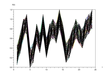
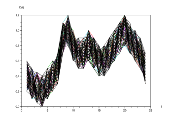
The initial state follows a uniform probability law over . We also draw particles for the initial state and each one is associated with the previous trajectories with the same index to form one scenario among . The control random variables are subject for each to the bounds .
The mapping modelling the electricity production is chosen to represent a linear variation between and with respect to the water fall height :
The expression of the instantaneous cost is
where is the electricity price at stage . The variation of this price is depicted in Figure 4.
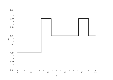
The final cost is an incentive to fill the dam at the end of the day:
4.3 Results using Dynamic Programming
We apply Algorithm 2 to Problem (31b) using an even discretization of the state space in points:
The two operators and are linear interpolation operators: to compute the value of a function outside the grid, we consider the weighted mean of the two surrounding grid points. The optimal feedback laws obtained at each time stage will be used as a reference in the comparison with the other resolution methods. The optimal cost is obtained by simulating the system using the optimal feedback laws over all trajectories:
| (32) |
4.4 Results obtained by Stochastic Programming
We then make use of a stochastic programming technique to solve Problem (31b). Using quantization techniques, we first generate a scenario tree from the noises trajectories. We will not discuss here the quantization method used to build such a scenarios tree and refer to [2] for further details. The resulting tree includes nodes at stage , nodes at stage and so on till stage for which we have nodes. As , the tree structure becomes deterministic as soon as , each node in the tree corresponding to having a unique future (Figure 1 just sketches the beginning of the story).
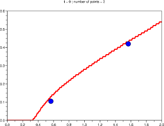
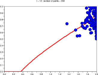
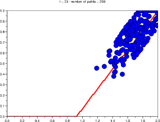
Problem (31b) is then formulated and optimized over the tree: the optimization process yields a pair of optimal values for the state and the control at each node of the tree. The next figures depict the optimal pairs of particles at different time stages (represented by dots) and the optimal feedback laws obtained by Dynamic Programming (represented by continuous curves). The comparison leads to the following conclusions.
-
•
There are only two nodes corresponding to in the scenario tree, and therefore only two optimal control particles. These two particles fit the optimal feedback obtained by Dynamic Programming rather accurately (see Figure 6), but it would be difficult to synthesize a feedback law with such a limited number of points.
- •
4.5 Results with the adaptive mesh method
We ultimately apply Algorithm 3 to solve the hydro-electric dam management problem (31b). The result of this algorithm is an optimal feedback law for every time stage . We then draw new noise trajectories independent from those used by the algorithm, and we simulate the system behavior along these new trajectories using the optimal feedback laws:
and thus obtain an approximation of the optimal cost generated by this algorithm:
This optimal cost is close to the cost generated by Dynamic Programming. We are also interested in the controls generated by the adaptive mesh method. To this purpose, Figures 9, 9 and 10 show the optimal control particles given by the adaptive mesh method (dots), to be compared with the optimal feedback laws obtained by Dynamic Programming (curves) for different time stages.
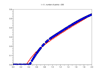
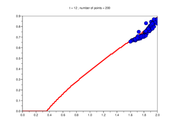
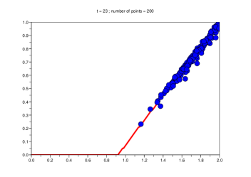
We note that the optimal particles obtained by the adaptive mesh method are close to the feedback laws obtained by Dynamic Programming. By construction, there are the same number of particles at each time stage , and the dispersion of the particles remains at first sight constant from the beginning to the end of the time horizon. This represents a significant advance compared to the scenario tree method. On the other hand, observe that particles may sometimes concentrate in restricted parts of the state space (see Figure 9): in our view, this is not a drawback, but an advantage of the proposed method in that the optimal feedback is computed only where it is needed to do so. Indeed, the particles distribute adaptively and automatically according to the optimal probability density of the state (we call this an “adaptive mesh” — in Figure 9, the distribution is even because the initial condition is uniformly distributed), and this is an advantage over Dynamic Programming in which a uniform grid is defined a priori over the whole state space, irrespective of the optimal solution distribution.
5 Conclusions and perspectives
In this paper we presented new tractable methods for solving stochastic optimal control problems in the discrete time case. We derived several forms of the optimality conditions for such problems:
- •
-
•
in the Markovian case, non-adapted optimality conditions (19) and adapted optimality conditions (20) with measurability constraints on the state variable; the conditional expectations are taken with respect to the instantaneous state variable whose dimension is constant over the time stages, but the mean square error when approximating such conditional expectations depends on the state space dimension;
-
•
still in the Markovian case, functional optimality conditions (21) including only expectations.
The last conditions have been used to devise a gradient-like adaptive mesh algorithm in order to solve stochastic optimal control problems in the Markovian case, and we applied the algorithm to a hydro-electric dam management problem.
In light of the numerical results, it is clear that the proposed adaptive mesh algorithm represents a significant advance with respect to usual stochastic programming techniques (same number of particles and same particle dispersion at every time stage). In addition, the adaptive mesh feature may save useless computations in some problems, depending on the profile of the optimal state probability density. In fact, the only a priori discretization concerns noise particles, which does not depend on the dimension of the underlining state space: the only operator which could be dimension-dependent is the interpolation operator.
Future work will concentrate on the convergence rate of the mesh algorithm with respect to the number of noise trajectories. We will also deal with stochastic optimal control problems involving a multi-dimensional state vector, and try to quantify the impact of the interpolation operator on the approximation error.
Appendix A Optimization on an Hilbert space: a special case
Let be an Hilbert space, let be a closed convex subset of and let be a real valued function defined on . We consider the following optimization problem:
| (33) |
In the following, will denote the indicator function of a subset , namely
The optimization literature gives different expressions for the necessary optimality conditions of an optimization problem in a general Hilbert space (see e.g. [11]). For instance, if is solution of (33), then the following statements are equivalent:
| (34a) | |||
| (34b) | |||
| (34c) | |||
We now consider a specific structure for the feasible set . More precisely, we assume that , being a closed subspace of and being a closed convex subset of . We moreover assume that the following property holds.
Assumption 5.
The sets and are such that .
Then the projection operator on has the following property.
Lemma 12.
Under Assumption 5, the following relation holds true:
Proof.
Let . Then
From the characterization of the projection of over the convex subset , the last inner product in the previous expression is non positive: therefore,
From , we deduce that . Since is a self-adjoint operator, we have
the last inequality arising from the fact that (since is a linear subspace, then is a linear operator). We thus conclude that, for all ,
a variational inequality which characterizes as the projection of over . ∎
The following proposition gives necessary optimality conditions for Problem (33) when the feasible set has the specific structure .
Proposition 13.
References
- [1] J.-P. Aubin and H. Frankowska, Set-valued Analysis, Birkhäuser, Boston, 1990.
- [2] K. Barty, Contributions à la discrétisation des contraintes de mesurabilité pour les problèmes d’optimisation stochastique, PhD dissertation, École Nationale des Ponts et Chaussées, 2004.
- [3] K. Barty, P. Carpentier, J.-P. Chancelier, G. Cohen, M. De Lara, and T. Guilbaud, Dual effect free stochastic controls, Annals of Operations Research, 142 (2006), pp. 41–62.
- [4] R. Bellman, Dynamic Programming, Princeton University Press, New Jersey, 1957.
- [5] D. Bertsekas, Dynamic programming and stochastic control, Acad. Press, 1976.
- [6] D. Bertsekas and S. Shreve, Stochastic Optimal Control: the discrete-time case, Athena Scientific, Belmont, 1996.
- [7] L. Breiman, Probability, Society for Industrial and Applied Mathematics, Philadelphia PA, 1992.
- [8] P. Brodie, M. Glasserman, A stochastic mesh method for pricing high dimensional american options, The journal of computational finance, 7 (2004).
- [9] A. Dallagi, Méthodes particulaires en commande optimale stochastique, PhD dissertation, Université Paris I Panthéon-Sorbonne, 2007.
- [10] J. Dupac̀ová, N. Gröwe-Kuska, and W. Römisch, Scenario reduction in stochastic programming. An approach using probability metrics, Math. Program., 95 (2003), pp. 493–511.
- [11] I. Ekeland and R. Temam, Convex analysis and variational problems, SIAM, Philadelphia, 1999.
- [12] H. Heitsch and W. Römisch, Scenario reduction algorithms in stochastic programming, Comput. Optim. Appl., (2003), pp. 187–206.
- [13] J.-B. Hiriart-Urruty, Extension of lipschitz integrands and minimization of nonconvex integral functionals : Applications to the optimal recourse problem in dicrete time, Probability and mathematical statistics, 3 (1982), pp. 19–36.
- [14] S. Leese, Multifunctions of Souslin type, Bull. Austral. Math. Soc., 11 (1974), pp. 395–411.
- [15] J. Outrata and W. Römisch, On optimality conditions for some nonsmooth optimization problems over spaces, Journal of Optimization Theory and Applications, 126 (2005), pp. 411–438.
- [16] G. Pflug, Scenario tree generation for multiperiod financial optimization by optimal discretization, Math. Program., 89 (2001), pp. 251–271.
- [17] M. Rao, Measure Theory and Integration, Pure and Applied Mathematics Series, Marcel Dekker Inc, 2004.
- [18] R. Rockafellar and R.-B. Wets, Variational Analysis, Springer Verlag, Berlin Heidelberg, 1998.
- [19] C. Strugarek, Approches variationnelles et autres contributions en optimisation stochastique, PhD dissertation, École Nationale des Ponts et Chaussées, 2006.
- [20] J. Thénié and J. Vial, Step decision rules for multistage stochastic programming: a heuristic approach. http://www.optimization-online.org/DB_HTML/2006/08/1440.html, 2006.
- [21] D. Wagner, Survey of measurable selection theorems, SIAM J. Control Optim., 15 (1977), pp. 859–903.