Statistical Properties of Turbulence: An Overview

Abstract

We present an introductory overview of several challenging problems in the statistical characterisation of turbulence. We provide examples from fluid turbulence in three and two dimensions, from the turbulent advection of passive scalars, turbulence in the one-dimensional Burgers equation, and fluid turbulence in the presence of polymer additives.

1. Introduction

Turbulence is often described as the last great unsolved problem of classical physics  [?,?,?]. However, it is not easy to state what would constitute a solution of the turbulence problem. This is principally because turbulence is not one problem but a collection of several important problems: These include the characterisation and control of turbulent flows, both subsonic and supersonic, of interest to engineers such as flows in pipes or over cars and aeroplanes  [?,?]. Mathematical questions in this area are concerned with developing proofs of the smoothness, or lack thereof, of solutions of the Navier-Stokes and related equations  [?,?,?,?,?]. Turbulence also provides a variety of challenges for fluid dynamicists  [?,?,?,?], astrophysicists  [?,?,?,?], geophysicists  [?,?], climate scientists  [?], plasma physicists  [?,?,?,?,?], and statistical physicists  [?,?,?,?,?,?,?,?,?,?]. In this brief overview, written primarily for physicists who are not experts in turbulence, we concentrate on some recent advances in the statistical characterisation of fluid turbulence  [?] in three dimensions, the turbulence of passive scalars such as pollutants  [?], two-dimensional turbulence in thin films or soap films  [?,?], turbulence in the Burgers equation  [?,?,?], and fluid turbulence with polymer additives  [?,?,?]; in most of this paper we restrict ourselves to homogeneous, isotropic turbulence   [?,?,?]; and we highlight some similarities between the statistical properties of systems at a critical point and those of turbulent fluids  [?,?,?]. Several important problems that we do not attempt to cover include Rayleigh-Bénard turbulence  [?], superfluid turbulence  [?,?], magnetohydrodyanmic turbulence  [?,?,?,?], the behaviour of inertial particles in turbulent flows  [?], the transition to turbulence in different experimental situations  [?,?], and boundary-layer  [?,?] and wall-bounded  [?] turbulence.

This paper is organised as follows: Section 2 gives an overview of some of the experiments of relevance to our discussion here. In Section 3 we introduce the equations that we consider. Section 4 is devoted to a summary of phenomenological approaches that have been developed, since the pioneering studies of Richardson  [?] and Kolmogorov  [?], in 1941 (K41), to understand the behaviour of velocity and other structure functions in inertial ranges. Section 5 introduces the ideas of multiscaling that have been developed to understand deviations from the predictions of K41-type phenomenology. Section 6 contains illustrative direct numerical simulations; it consists of five subsections devoted to (a) three-dimensional fluid turbulence, (b) shell models, (c) two-dimensional turbulence in soap films, (d) turbulence in the one-dimensional Burgers equation, and (e) fluid turbulence with polymer additives. Section 7 contains concluding remarks.

2. Experimental Overview

Turbulent flows abound in nature. They include the flow of water in a garden pipe or in rapids, the flow of air over moving cars or aeroplanes, jets that are formed when a fluid is forced through an orifice, the turbulent advection of pollutants such as ash from a volcanic eruption, terrestrial and Jovian storms, turbulent convection in the sun, and turbulent shear flows in the arms of spiral galaxies. A wide variety of experimental studies have been carried out to understand the properties of such turbulent flows; we concentrate on those that are designed to elucidate the statistical properties of turbulence, especially turbulence that is, at small spatial scales and far away from boundaries, homogeneous and isotropic. Most of our discussion will be devoted to incompressible flows, i.e., low-Mach-number cases in which the fluid velocity is much less than the velocity of sound in the fluid.

In laboratories such turbulence is generated in many different ways. A common method uses a grid in a wind tunnel  [?]; the flow downstream from this grid is homogeneous and isotropic, to a good approximation. Another technique use the von Kármán swirling flow, i.e., flow generated in a fluid contained in a cylindrical tank with two coaxial, counterrotating discs at its ends  [?,?,?]; in the middle of the tank, far away from the discs, the turbulent flow is approximately homogeneous and isotropic. Electromagnetically forced thin films and soap films  [?,?,?] have yielded very useful results for two-dimensional turbulence. Turbulence data can also be obtained from atmospheric boundary layers  [?,?,?,?], oceanic flows  [?], and astrophysical measurements  [?]; experimental conditions cannot be controlled as carefully in such natural settings as they can be in a laboratory, but a far greater range of length scales can be probed than is possible in laboratory experiments.

Traditionally, experiments have measured the velocity ${\bf u}({\bf x},t)$ at a single point ${\bf x}$ at various times $t$ by using hot-wire anemometers; these anemometers can have limitations in (a) the number of components of the velocity that can be measured and (b) the spatial and temporal resolutions that can be obtained  [?,?]. Such measurements yield a time series for the velocity; if the mean flow velocity $U>>u_{rms}$, the root-mean-square fluctuations of the velocity, then Taylor’s frozen-flow hypothesis  [?,?] can be used to relate temporal separations $\delta t$ to spatial separations $\delta r$, along the mean flow direction via $\delta r=U\delta t$. The Reynolds number $Re=UL/\nu$, where $U$ and $L$ are typical velocity and length scales in the flow and $\nu$ is the kinematic viscosity, is a convenient dimensionless control parameter; at low $Re$ flows are laminar; as it increases increases there is a transition to turbulence often via a variety of instabilities  [?] that we will not cover here; and at large $Re$ fully developed turbulence sets in. To compare different flows it is often useful to employ the Taylor-microscale Reynolds number $Re_{\lambda}=u_{rms}\lambda/\nu$, where the Taylor microscale $\lambda$ can be obtained from the energy spectrum as described below (Sec. 6.3).

Refinements in hot-wire anemometry  [?,?] and flow visualisation techniques such as laser-doppler velocimetry (LDV)  [?], particle-image velocimetry (PIV)  [?,?], particle-tracking velocimetry (PTV)  [?,?], tomographic PIV  [?], holographic PIV  [?], and digital holographic microscopy  [?] have made it possible to obtain reliable measurements of the Eulerian velocity ${\bf u}({\bf x},t)$ (see Sec. 3) in a turbulent flow. In the simplest forms of anemometry a time series of the velocity is obtained at a given point in space; in PIV two components of the velocity field can be obtained in a sheet at a given time; holographic PIV can yield all components of the velocity field in a volume. Components of the velocity derivative tensor $A_{ij}\equiv\partial_{j}u_{i}$ can also be obtained  [?] and thence quantities such as the energy dissipation rate per unit mass per unit volume $\epsilon\equiv-\nu\sum_{i,j}(\partial_{i}u_{j}+\partial_{j}u_{i})^{2}$, the vorticity $\omega=\nabla\times{\bf u}$, and components of the rate of strain tensor $s_{ij}\equiv(\partial_{i}u_{j}+\partial_{j}u_{i})/2$, where the subscripts $i$ and $j$ are Cartesian indices. A discussion of the subtleties and limitations of these measurement techniques lies beyond the scope of our overview; we refer the reader to Refs.  [?,?,?] for details. Significant progress has also been made over the past decade in the measurement of Lagrangian trajectories (see Sec. 3) of tracer particles in turbulent flows  [?,?]. Given such measurements, experimentalists can obtain several properties of turbulent flows. We give illustrative examples of the types of properties we consider.

Flow-visualisation methods often display large-scale coherent structures in turbulent flows. Examples of such structures plumes in Rayleigh-Bérnard convection  [?], structures behind a splitter plate  [?], and large vortical structures in two-dimensional or stratified flows  [?,?,?]. In three-dimensional flows, as we will see in greater detail below, energy that is pumped into the flow at the injection scale $L$ cascades, as first suggested by Richardson  [?], from large-scale eddies to small-scale ones till it is eventually dissipated around and beyond the dissipation scale $\eta_{d}$. By contrast, two-dimensional turbulence  [?,?,?,?] displays a dual cascade: there is an inverse cascade of energy from the scale at which it is pumped into the system to large length scales and a direct cascade of enstrophy $\Omega=\langle\frac{1}{2}\omega^{2}\rangle$ to small length scales. The inverse cascade of energy is associated with the formation of a few large vortices; in practical realisations the sizes of such vortices are controlled finally by Ekman friction that is induced, e.g., by air drag in soap-film turbulence.

Measurements of the vorticity $\omega$ in highly turbulent flows show that regions of large $\omega$ are organised into slender tubes. The first experimental evidence for this was obtained by seeding the flow with bubbles that moved preferentially to regions of low pressure  [?] that are associated with large-$\omega$ regimes. For recent experiments on vortex tubes we refer the reader to Ref.  [?].

The time series of the fluid velocity at a given point ${\bf x}$ shows strong fluctuations. It is natural, therefore, to inquire into the statistical properties of turbulent flows. From the Eulerian velocity ${\bf u}({\bf x},t)$ and its derivatives we can obtain one-point statistics, such as probability distribution functions (PDFs) of the velocity and its derivatives. Velocity PDFs are found to be close to Gaussian distributions. However, PDFs of $\omega^{2}$ and velocity derivatives show significant non-Gaussian tails; for a recent study, which contains references to earlier work, see Ref.  [?]. The PDF of $\epsilon$ is non-Gaussian too and the time series of $\epsilon$ is highly intermittent  [?]; furthermore, in the limit $Re\to\infty$, i.e., $\nu\to 0$, the energy dissipation rate per unit volume $\epsilon$ approaches a positive constant value (see, e.g., Fig. 2 of Ref.  [?]), a result referred to as a dissipative anomaly or the zeroth law of turbulence.

Various statistical properties of the rate-of-strain tensor, with components $s_{ij}$, have been measured  [?]. The eigenvalues $\lambda_{1},\,\lambda_{2},$ and $\lambda_{3}$, with $\lambda_{1}>\lambda_{2}>\lambda_{3}$ , of this tensor must satisfy $\lambda_{1}+\lambda_{2}+\lambda_{3}=0$, with $\lambda_{1}>0$ and $\lambda_{2}<0$, in an incompressible flow. The sign of $\lambda_{2}$ cannot be determined by this condition but its PDF shows that, in turbulent flows, $\lambda_{2}$ has a small, positive mean value  [?]; and the PDFs of $\cos(\omega\cdot e_{i})$, where $e_{i}$ is the normalised eigenvector corresponding to $\lambda_{i}$, show that there is a preferential alignment  [?] of $\omega$ and $e_{2}$. Joint PDFs can be measured too with good accuracy. An example of recent interest is a tear-drop feature observed in contour plots of the joint PDF of, respectively, the second and third invariants, $Q=-tr(A^{2})/2$ and $R=-tr(A^{3})/3$ of the velocity gradient tensor $A_{ij}$ (see Fig. 11 of Ref.  [?]); we display such a plot in Sec. 6 that deals with direct numerical simulations.

Two-point statistics are characterised conventionally by studying the equal-time, order-$p$, longitudinal velocity structure function

$$S_{p}({\bf r})=\langle[(u({\bf x}+{\bf r})-u({\bf x}))\cdot({\bf r}/r]^{p}\rangle,$$ (1)

where the angular brackets indicate a time average over the nonequilibrium statistical steady state that we obtain in forced turbulence (decaying turbulence is discussed in Sec. 6.2). Experiments  [?,?] show that, for separations $r$ in the inertial range $\eta_{d}<<r<<L$,

$$S_{p}({\bf r})\sim r^{\zeta_{p}},$$ (2)

with exponents $\zeta_{p}$ that deviate significantly from the simple scaling prediction  [?] $\zeta_{p}^{K41}=p/3$, especially for $p>3$, where $\zeta_{p}<\zeta_{p}^{K41}$. This prediction, made by Kolmogorov in 1941 (hence the abbreviation K41), is discussed in Sec. 4 below; the deviations from this simple scaling prediction are referred to as multiscaling (Sec. 5) and they are associated with the intermittency of $\epsilon$ mentioned above. We mention, in passing, that the log-Poisson model due to She and Leveque provides a good parametrisation of the plot of $\zeta_{p}$ versus $p$   [?].

The second-order structure function $S_{2}({\bf r})$ can be related easily by Fourier transformation to the the energy spectrum $E(k)=4\pi k^{2}\langle|{\tilde{\bf u}}(k)|^{2}\rangle$, where the tilde denotes the Fourier transform, $k=|{\bf k}|$, ${\bf k}$ is the wave vector, we assume that the turbulence is homogeneous and isotropic, and, for specificity, we give the formula for the three-dimensional case. Since $\zeta_{2}^{K41}=2/3$, the K41 prediction is

$$E^{K41}(k)\sim k^{-5/3},$$ (3)

a result that is in good agreement with a wide range of experiments [see, e.g., Refs.  [?,?]].

The structure functions $S_{p}(r)$ are the moments of the PDFs of the longitudinal velocity increments $\delta u_{||}\equiv[(u({\bf x}+{\bf r})-u({\bf x}))\cdot({\bf r}/r)]$. [In the argument of $S_{p}$ we use $r$ instead of ${\bf r}$ when we consider homogeneous, isotropic turbulence.] These PDFs have been measured directly  [?] and they show non-Gaussian tails; as $r$ decreases, the deviations of these PDFs from Gaussian distributions increases.

We now present a few examples of recent Lagrangian measurements  [?,?] that have been designed to track tracer particles in, e.g., the von Kármán flow at large Reynolds numbers. By employing state-of-the-art measurement techniques, such as silicon strip detectors  [?], used in high-energy-physics experiments, or acoustic-doppler methods  [?], these experiments have been able to attain high spatial resolution and high sampling rates and have, therefore, been enable to obtain good data for acceleration statistics of Lagrangian particles and the analogues of velocity structure functions for them.

These experiments  [?] find, for $500<Re_{\lambda}<970$, consistency with the Heisenberg-Yaglom scaling form of the acceleration variance, i.e.,

$$\langle a_{i}a_{j}\rangle\sim\epsilon^{(3/2)}\nu^{(-1/2)}\delta_{ij},$$ (4)

where $a_{i}$ is the Cartesian component $i$ of the acceleration. Furthermore, there are indications of strong intermittency effects in the acceleration of particles and anisotropy effects are present even at very large $Re_{\lambda}$.

Order-$p$ Lagrangian velocity structure functions are defined along a Lagrangian trajectory as

$$S^{L}_{i,p}(\tau)=\langle[v^{L}_{i}(t+\tau)-v^{L}_{i}(t)]^{p}\rangle,$$ (5)

where the superscript $L$ denotes Lagrangian and the subscript $i$ the Cartesian component. If the time lag $\tau$ lies in the temporal analogue of the inertial range, i.e., $\tau_{\eta}\ll\tau\ll T_{L}$, where $\tau_{\eta}$ is the viscous dissipation time scale and $T_{L}$ is the time associated with the scale $L$ at which energy is injected into the system, then it is expected that

$$S^{L}_{i,p}(\tau)\sim\tau^{\zeta^{L}_{i,p}}.$$ (6)

The analogue of the dimensional K41 prediction is $\zeta^{L,K41}_{i,p}=p/2$; experiments and simulations  [?] indicate that there are corrections to this simple dimensional prediction.

The best laboratory realisations of two-dimensional turbulence are (a) a thin layer of a conducting fluid excited by magnetic fields, varying both in space and time and applied perpendicular to the layer  [?], and (b) soap films  [?] in which turbulence can be generated either by electromagnetic forcing or by the introduction of a comb, which plays the role of a grid, in a rapidly flowing soap film. In the range of parameters used in typical experimental studies  [?,?,?,?] both these systems can be described quite well  [?,?] by the 2D Navier Stokes equation (see Sec. 3) with an additional Ekman-friction term, induced typically by air drag; however, in some cases we must also account for corrections arising from fluctuations of the film thickness, compressibility effects, and the Marangoni effect. Measurement techniques are similar to those employed to study three-dimensional turbulence  [?,?,?]. Two-dimensional analogues of the PDFs described above for 3D turbulence have been measured [see, e.g., Refs.  [?]]; we will touch on these briefly when we discuss numerical simulations of 2D turbulence in Sec. 6.3. Velocity and vorticity structure functions can be measured as in 3D turbulence; however, inertial ranges associated with inverse and forward cascades must be distinguished; the former shows simple scaling with an energy spectrum $E(k)\sim k^{-5/3}$ whereas the latter has an energy spectrum $E(k)\sim k^{-(3+\delta)}$, with $\delta=0$ if there is no Ekman friction and $\delta>0$ otherwise. In the forward cascade velocity structure functions show simple scaling  [?]; we are not aware of experimental measurements of vorticity structure functions (we will discuss these in the context of numerical simulations in Sec. 6.3).

We end this Section with a brief discussion of one example of turbulence in a non-Newtonian setting, namely, fluid flow in the presence of polymer additives. There are two dimensionless control parameters in this case: $Re$ and the Weissenberg number $We$, which is a ratio of the polymer-relaxation time and a typical shearing time in the flow (some studies  [?] use a similar dimensionless parameter called the Deborah number $De$). Dramatically different behaviours arise depending on the values of these parameters.

In the absence of polymers the flow is laminar at low $Re$; however, the addition of small amounts of high-molecular-weight polymers can induce elastic turbulence  [?], i.e., a mixing flow that is like turbulence and in which the drag increases with increasing $We$. We will not discuss elastic turbulence in detail here; we refer the reader to Ref.  [?] for an overview of experiments and to Ref.  [?] for representative numerical simulations.

If, instead, the flow is turbulent in the absence of polymers, i.e., we consider large-$Re$ flows, then the addition of polymers leads to the dramatic phenomenon of drag reduction that has been known since 1949  [?]; it has obvious and important industrial applications  [?,?,?,?,?]. Normally drag reduction is discussed in the context of pipe or channel flows: on the addition of polymers to turbulent flow in a pipe, the pressure difference required to maintain a given volumetric flow rate decreases, i.e., the drag is reduced and a percentage drag reduction can be obtained from the percentage reduction in the pressure difference. For a recent discussion of drag reduction in pipe or channel flows we refer the reader to Ref.  [?]. Here we concentrate on other phenomena that are associated with the addition of polymers to turbulent flows that are homogeneous and isotropic. In particular, experiments  [?] show that the polymers lead to a suppression of small-scale structures and important modifications in the second-order structure function  [?]. We will return to an examination of such phenomena when we discuss direct numerical simulations in Sec. 6.5.

3. Models

Before we discuss advances in the statistical characterization of turbulence, we provide a brief description to the models we consider. We start with the basic equations of hydrodynamics, in three and two dimensions, that are central to studies of turbulence. We also give introductory overviews of the Burgers equation in one dimension, the advection-diffusion equation for passive scalars, and the coupled NS and finitely extensible nonlinear elastic Peterlin (FENE-P) equations for polymers in a fluid. We end this Section with a description of shell models that are often used as highly simplified models for homogeneous, isotropic turbulence.

At low Mach numbers, fluid flows are governed by the Navier-Stokes (NS) Eq. (7) augmented by the incompressibility condition

$$\partial_{t}{\bf u}+({\bf u.}\nabla){\bf u} = -\nabla p+\nu\nabla^{2}{\bf u}+{\bf f},$$ (7)

$$\nabla\cdot{\bf u} = 0,$$ (8)

where we use units in which the density $\rho$ = 1, the Eulerian velocity at point ${\bf r}$ and time $t$ is ${\bf u}({\bf r},t)$, the external body force per unit volume is ${\bf f}$ , and $\nu$ is the kinematic viscosity. The pressure $p$ can be eliminated by using the incompressibility condition  [?,?,?] and it can then be obtained from the Poisson equation $\nabla^{2}p=-\partial_{ij}(u_{i}u_{j})$. In the unforced, inviscid case, the momentum, the kinetic energy, and the helicity $H\equiv\int d{\bf r}\omega\cdot{\bf u}/2$ are conserved; here $\omega\equiv\nabla\times{\bf u}$ is the vorticity. The Reynolds number $Re\equiv LV/\nu$, where $L$ and $V$ are characteristic length and velocity scales, is a convenient dimensionless control parameter: The flow is laminar at low $Re$ and irregular, and eventually turbulent, as $Re$ is increased.

In the vorticity formulation the NS equation 8 becomes

$$\partial_{t}{\bf\omega}=\nabla\times{\bf u}\times{\bf\omega}+\nu\nabla^{2}{\bf\omega}+\nabla\times{\bf f};$$ (9)

the pressure is eliminated naturally here. This formulation is particularly useful is two dimensions since $\omega$ is a pseudo-scalar in this case. Specifically, in two dimensions, the NS equation can be written in terms of $\omega$ and the stream function $\psi$:

$$\partial_{t}\omega-J(\psi,\omega) = \nu\nabla^{2}\omega+\alpha_{E}\omega+f;$$ (10)

$$\nabla^{2}\psi = \omega;$$ (11)

$$J(\psi,\omega) \equiv (\partial_{x}\psi)(\partial_{y}\omega)-(\partial_{x}\omega)(\partial_{y}\psi).$$ (12)

Here $\alpha_{E}$ is the coefficient of the air-drag-induced Ekman-friction term. The incompressibility constraint

$$\partial_{x}u_{x}+\partial_{y}u_{y}=0$$ (13)

ensures that the velocity is uniquely determined by $\psi$ via

$${\bf u}\equiv(-\partial_{y}\psi,\partial_{x}\psi).$$ (14)

In the inviscid, unforced case we have more conserved quantities in two dimensions than in three; the additional conserved quantities are $\langle\frac{1}{2}\omega^{n}\rangle$, for all powers $n$, the first of which is the mean enstrophy, $\Omega=\langle\frac{1}{2}\omega^{2}\rangle$.

In one dimension (1D) the incompressibility constraint leads to trivial velocity fields. It is fruitful, however, to consider the Burgers equation  [?], which is the NS equation without pressure and the incompressibility constraint. This has been studied in great detail as it often provides interesting insights into fluid turbulence. In 1D the Burgers equation is

$$\partial_{t}v+v\partial_{x}v=\nu\nabla^{2}v+f,$$ (15)

where $f$ is the external force and the velocity $v$ can have shocks since the system is compressible. In the unforced, inviscid case the Burgers equation has infinitely many conserved quantities, namely, $\int v^{n}dx$ for all integers $n$. In the limit $\nu\rightarrow 0$ we can use the Cole-Hopf transformation, $v=\partial_{x}\Psi$, $f\equiv-\partial_{x}F$, and $\Psi\equiv 2\nu\ln\Theta$, to obtain $\partial_{t}\Theta=\nu\partial_{x}^{2}\Theta+F\Theta/(2\nu)$, a linear partial differential equation (PDE) that can be solved explicitly in the absence of any boundary  [?,?].

Passive scalars such as pollutants can be advected by fluids. These flows are governed by the advection-diffusion equation

$$\partial_{t}\theta+{\bf u}.\nabla\theta=\kappa\nabla^{2}\theta+{\bf f}_{\theta},$$ (16)

where $\theta$ is the passive-scalar field, the advecting velocity field u satisfies the NS equation 8, and ${\bf f}_{\theta}$ is an external force. The field $\theta$ is passive because it does not act on or modify ${\bf u}$. Note that Eq.( 16) is linear in $\theta$. It is possible, therefore, to make considerable analytical progress in understanding the statistical properties of passive-scalar turbulence for the simplified model of passive-scalar advection due to Kraichnan  [?,?]; in this model each component of ${\bf f}_{\theta}$ is a zero-mean Gaussian random variable that is white in time; furthermore, each component of ${\bf u}$ is taken to be a zero-mean Gaussian random variable that is white in time and which has the covariance

$$\left\langle u_{i}({\bf x},t)u_{j}({\bf x}+{\bf r},t^{\prime})\right\rangle=2D_{ij}\delta(t-t^{\prime});$$ (17)

the Fourier transform of $D_{ij}$ has the form

$$\tilde{D}_{ij}({\bf q})\propto{\big{(}}q^{2}+\frac{1}{L^{2}}{\big{)}}^{-(d+\xi)/2}e^{-\eta q^{2}}{\big{[}}\delta_{ij}-\frac{q_{i}q_{j}}{q^{2}}{\big{]}};$$ (18)

q is the wave vector, $L$ is the characteristic large length scale, $\eta$ is the dissipation scale, and $\xi$ is a parameter. In the limit of $L\to\infty$ and $\eta\to 0$ we have, in real space,

$$D_{ij}({\bf r})=D^{0}\delta_{ij}-\frac{1}{2}d_{ij}({\bf r})$$ (19)

with

$$d_{ij}=D_{1}r^{\xi}\big{[}(d-1+\xi)\delta_{ij}-\xi\frac{r_{i}r_{j}}{r^{2}}\big{]}.$$ (20)

$D_{1}$ is a normalization constant and $\xi$ a parameter; for $0<\xi<2$ equal-time passive-scalar structure functions show multiscaling  [?].

We turn now to an example of a model for non-Newtonian flows. This model combines the NS equation for a fluid with the finitely extensible nonlinear elastic Peterlin (FENE-P) model for polymers; it is used inter alia to study the effects of polymer additives on fluid turbulence. This model is defined by the following equations:

$$\partial_{t}{\bf u}+({\bf u}.{\bf\nabla}){\bf u} = \nu\nabla^{2}{\bf u}+\frac{\mu}{\tau_{P}}\nabla.[f(r_{P}){\cal C}]-{\nabla}p;$$ (21)

$$\partial_{t}{\cal C}+{\bf u}.{\bf\nabla}{\cal C} = {\cal C}.(\nabla{\bf u})+{(\nabla{\bf u})^{T}}.{\cal C}-\frac{{f(r_{P}){\cal C}}-{\cal I}}{\tau_{P}}.$$ (22)

Here $\nu$ is the kinematic viscosity of the fluid, $\mu$ the viscosity parameter for the solute (FENE-P), $\tau_{P}$ the polymer relaxation time, $\rho$ the solvent density, $p$ the pressure, $(\nabla{\bf u})^{T}$ the transpose of $({\nabla{\bf u}})$, ${\cal C}_{\alpha\beta}\equiv{\langle{R_{\alpha}}{R_{\beta}}\rangle}$ the elements of the polymer-conformation tensor ${\cal C}$ (angular brackets indicate an average over polymer configurations), ${\cal I}$ the identity tensor with elements $\delta_{\alpha\beta}$, $f(r_{P})\equiv{(L^{2}-3)/(L^{2}-r_{P}^{2})}$ the FENE-P potential that ensures finite extensibility, $r_{P}\equiv\sqrt{Tr(\cal C)}$ and $L$ the length and the maximum possible extension, respectively, of the polymers, and $c\equiv\mu/(\nu+\mu)$ a dimensionless measure of the polymer concentration  [?].

The hydrodynamical partial differential equations (PDEs) discussed above are difficult to solve, even on computers via direct numerical simulation (DNS), if we want to resolve the large ranges of spatial and temporal scales that become relevant in turbulent flows. It is useful, therefore, to consider simplified models of turbulence that are numerically more tractable than these PDEs. Shell models are important examples of such simplified models; they have proved to be useful testing grounds for the multiscaling properties of structure functions in turbulence. We will consider, as illustrative examples, the Gledzer-Ohkitani-Yamada (GOY) shell model  [?] for fluid turbulence in three dimensions and a shell model for the advection-diffusion equation  [?].

Shell models cannot be derived from the NS equation in any systematic way. They are formulated in a discretised Fourier space with logarithmically spaced wave vectors $k_{n}=k_{0}{\tilde{\lambda}}^{n}\/,{\tilde{\lambda}}>1,$ associated with shells $n$ and dynamical variables that are the complex, scalar velocities $u_{n}\/$. Note that $k_{n}$ is chosen to be a scalar: spherical symmetry is implicit in GOY-type shell models since their aim is to study homogeneous, isotropic turbulence. Given that $k_{n}$ and $u_{n}$ are scalars, shell models cannot describe vortical structures or enforce the incompressibility constraint.

The temporal evolution of such a shell model is governed by a set of ordinary differential equations that have the following features in common with the Fourier-space version of the NS equation  [?]: they have a viscous-dissipation term of the form $-\nu k_{n}^{2}u_{n}$, they conserve the shell-model analogues of the energy and the helicity in the absence of viscosity and forcing, and they have nonlinear terms of the form $\imath k_{n}u_{n}u_{n^{\prime}}$ that couple velocities in different shells. In the NS equation all Fourier modes of the velocity affect each other directly but in most shell models nonlinear terms limit direct interactions to shell velocities in nearest- and next-nearest-neighbour shells; thus direct sweeping effects, i.e., the advection of the largest eddies by the the smallest eddies, are present in the NS equation but not in most shell models. This is why the latter are occasionally viewed as a highly simplified, quasi-Lagrangian representation (see below) of the NS equation.

The GOY-model evolution equations have the form

$$[\frac{d}{dt}+\nu k_{n}^{2}]u_{n}=i(a_{n}u_{n+1}u_{n+2}b_{n}u_{n-1}u_{n+1}+c_{n}u_{n-1}u_{n-2})^{\ast}+f_{n},$$ (23)

where complex conjugation is denoted by $\ast$, the coefficients are chosen to be $a_{n}=k_{n}$, $b_{n}=-\delta k_{n-1}$, $c_{n}=-(1-\delta)k_{n-2}$ to conserve the shell-model analogues of the energy and the helicity in the inviscid, unforced case; in any practical calculation $1\leq n\leq N$, where $N$ is the total number of shells and we use the boundary conditions $u_{n}=0\,\forall\,n<1$ or $\forall\,n>N$; as mentioned above $k_{n}={\tilde{\lambda}}^{n}k_{0}$ and many groups use ${\tilde{\lambda}}=2\/$, $\delta=1/2$, $k_{0}=1/16$, and $N=22$. The logarithmic discretisation here allows us to reach very high Reynolds number, in numerical simulations of this model, even with such a moderate value of $N$. For studies of decaying turbulence we set $f_{n}=0,\forall\,n$; in the case of statistically steady, forced turbulence  [?] it is convenient to use $f_{n}=(1+\imath)5\times 10^{-3}$. For such a shell model the analogue of a velocity structure function is $S_{p}(k_{n})=\langle|u(k_{n})|^{p}\rangle$ and the energy spectrum is $E(k_{n})=|u(k_{n})|^{2}/k_{n}$.

It is possible to construct other shell models, by using arguments similar to the ones we have just discussed, for other PDEs such as the advection-diffusion equation. Its shell-model version is

$$[\frac{d}{dt}+\kappa k_{n}^{2}]\theta=i[k_{n}(\theta_{n+1}u_{n-1}-\theta_{n-1}u_{n+1})-$$ (24)

$$\frac{k_{n-1}}{2}(\theta_{n-1}u_{n-2}+\theta_{n-2}u_{n-1})-$$ (25)

$$\frac{k_{n-1}}{2}(\theta_{n+2}u_{n+1}+\theta_{n+1}u_{n+2})]^{*}$$ (26)

For this model, the advecting velocity field can either be obtained from the numerical solution of a fluid shell model, like the GOY model above, or by using a shell-model version of the type of stochastic velocity field introduced in the Kraichnan model for passive-scalar advection  [?]. A shell-model analogue for the FENE-P model of fluid turbulence with polymer additives may be found in Ref.  [?].

3.1 Eulerian, Lagrangian, Quasi-Lagrangian frameworks

The Navier-Stokes Eq.( 8) is written in terms of the Eulerian velocity ${\bf u}$ at position ${\bf x}$ and time $t$; i.e., in the Eulerian case we use a frame of reference that is fixed with respect to the fluid; this frame can be used for any flow property or field. The Lagrangian framework  [?] uses a complementary point of view in which we fix a frame of reference to a fluid particle; this fictitious particle moves with the flow and its path is known as a Lagrangian trajectory. Each Lagrangian particle is characterised by its position vector ${\bf r_{0}}$ at time $t_{0}$; its trajectory at some later time $t$ is ${\bf R}={\bf R}(t;{\bf r_{0}},t_{0})$ and the associated Lagrangian velocity is

$${\bf v}=\biggl{(}\frac{d{\bf R}}{dt}\biggl{)}_{{\bf r_{0}}}.$$ (27)

We will also employ the quasi-Lagrangian  [?,?] framework that uses the following transformation for an Eulerian field $\psi({\bf r},t)$:

$${\hat{\psi}}({\bf r},t)\equiv\psi[{\bf r}+{\bf R}(t;{\bf r_{0}},0),t];$$ (28)

here ${\hat{\psi}}$ is the quasi-Lagrangian field and ${\bf R}(t;{\bf r_{0}},0)$ is the position at time $t$ of a Lagrangian particle that was at point ${\bf r_{0}}$ at time $t=0$.

As we have mentioned above, sweeping effects are present when we use Eulerian velocities. However, since Lagrangian particles move with the flow, such effects are not present in Lagrangian and quasi-Lagrangian frameworks. In experiments neutrally buoyant tracer particles are used to obtain Lagrangian trajectories that can be used to obtain statistical properties of Lagrangian particles.

4. Homogeneous Isotropic Turbulence: Phenomenology

In 1941 Kolmogorov  [?] developed his classic phenomenological approach to turbulence that is often referred to as K41. He used the idea of the Richardson cascade to provide an intuitive, though not rigorous, understanding of the power-law behaviours we have mentioned in Sec. 2. We give a brief introduction to K41 phenomenology and related ideas; for a detailed discussion the reader should consult Ref.  [?].

First we must recognise that there are two important length scales: (a) The large integral length scale $L$ that is comparable to the system size and at which energy injection takes place; flow at this scale depends on the details of the system and the way in which energy is injected into it; (b) and the small dissipation length scale $\eta_{d}$ below which energy dissipation becomes significant. The inertial range of scales, in which structure functions and energy spectra assume the power-law behaviours mentioned above (Sec. 2), lie in between $L$ and $\eta$; as $Re$ increases so does the extent of the inertial range.

In K41 Kolmogorov made the following assumptions: (a) Fully developed 3D turbulence is homogeneous and isotropic at small length scales and far away from boundaries. (b) In the statistical steady state, the energy dissipation rate per unit volume $\epsilon$ remains finite and positive even when $Re\to\infty$ (the dissipative anomaly mentioned above). (c) A Richardson-type cascade is set up in which energy is transferred by the breakdown of the largest eddies, created by inherent instabilities of the flow, to smaller ones, which decay in turn into even smaller eddies, and so on till the sizes of the eddies become comparable to $\eta_{d}$ where their energy can then be degraded by viscous dissipation. As $Re\to\infty$ all inertial-range statistical properties are uniquely and universally determined by the scale $r$ and $\epsilon$ and are independent of $L$, $\nu$ and $\eta_{d}$.

Dimensional analysis then yields the scaling form of the order-$p$ structure function

$$S_{p}^{K41}(r)\approx C\epsilon^{p/3}r^{p/3},$$ (29)

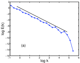
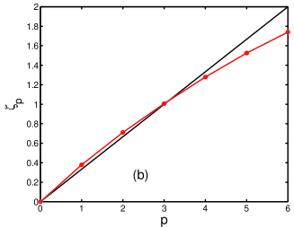
since $\epsilon$ has dimensions of $(length)^{2}(time)^{-3}$. [It is implicit here that the eddies, at any given level of the Richardson cascade, are space filling; if not, $\epsilon$ is intermittent and scale dependent as we discuss in Sec. 5 on multiscaling.] Thus $\zeta_{p}^{K41}=p/3$; for $p=2$ we get $S_{2}^{K41}(r)\sim r^{2/3}$ whose Fourier transform is related to the K41 energy spectrum $E(k)^{K41}\sim k^{-5/3}$ (left panel of Fig. 1).

The prediction $\zeta_{3}^{K41}=1$, unlike all others K41 results, can be derived exactly for the NS equation in the limit $Re\to\infty$. In particular, it can be shown that  [?,?]

$$S_{3}(\ell)\approx-\frac{4}{5}\epsilon\ell,$$ (30)

an important result, since it is both exact and nontrivial.

It is often useful to discuss K41 phenomenology by introducing $v_{\ell}$, the velocity associated with the inertial-range length scale $\ell$; clearly

$$v_{\ell}\sim\epsilon^{1/3}\ell^{1/3}.$$ (31)

The time scale $t_{\ell}\sim\frac{\ell}{v_{\ell}}$, the typical time required for the transfer of energy from scales of order $\ell$ to smaller ones. This yields the rate of energy transfer

$$\Pi\sim\frac{v^{2}_{\ell}}{t_{\ell}}\sim\frac{v^{3}_{\ell}}{\ell}.$$ (32)

Given the assumptions of K41, there is neither direct energy injection nor molecular dissipation in the inertial range. Therefore, the energy flux $\Pi$ becomes independent of $\ell$ and is equal to the mean energy dissipation rate $\epsilon$, which can now be written as

$$\epsilon\sim v^{3}_{\ell}/\ell.$$ (33)

A similar prediction, for the two-point correlations of a passive-scalar advected by a turbulent fluid is due to Obukhov and Corsin; we shall not discuss it here but refer the reader to Ref.  [?,?].

,

Figure  1.: (Color online) (a) A representative log-log plot of the energy spectrum $E(k)$ versus $k$, from a numerical simulation of the GOY shell model with 22 shells. The straight black line is a guide to the eye indicating K41 scaling $k^{-5/3}$. (b) A plot of the equal-time scaling exponents $\zeta_{p}$ versus $p$, with error bars, obtained from the GOY shell model. The straight black line (color online) indicates K41 scaling $p/3$.

As we have mentioned above, the cascade of energy in 3D turbulence is replaced in 2D turbulence by a dual cascade: an inverse cascade of energy from the injection scale to larger length scales and a forward cascade of enstrophy  [?,?,?,?]. In the inverse cascade the energy accumulation at large length scales is controlled eventually by Ekman friction. The analogue of K41 phenomenology for this case is based upon physical arguments due to Kraichnan, Leith and Batchelor  [?]. Given that there is energy injection at some intermediate length scale, kinetic energy get redistributed from such intermediate scales to the largest length scale. The scaling result for the two cascades gives us a kinetic energy spectrum that has a $k^{-5/3}$ form in the inverse-cascade inertial range and a $k^{-3}$ form (in the absence of Ekman friction) in the forward-cascade inertial range.

5. From scaling to multiscaling

In equilibrium statistical mechanics, equal-time and time-dependent correlation functions, in the vicinity of a critical point, display scaling properties that are well understood. For example, for a spin system in $d$ dimensions close to its critical point, the scaling forms of the equal-time correlation function $g(r;\bar{t},h)$ and its Fourier transform $\tilde{g}(k;\bar{t},h)$, for a pair of spins separated by a distance $r$, are as follows:

$$g(r;\bar{t},h)\approx\frac{G(r\bar{t}^{(\bar{\nu})},h/\bar{t}^{(\bar{\Delta})})}{r^{d-2+\bar{\eta}}};$$ (34)

$$\tilde{g}(k;\bar{t},h)\approx\frac{\tilde{G}(k/\bar{t}^{(\bar{\nu})},h/\bar{t}^{(\bar{\Delta})})}{k^{2-\bar{\eta}}}.$$ (35)

Here the reduced temperature $\bar{t}=(T-T_{c})/T_{c}$, where $T$ and $T_{c}$ are, respectively, the temperature and the critical temperature, and the reduced field $h=H/k_{B}T_{c}$, with $H$ the external field and $k_{B}$ the Boltzmann constant. The equal-time critical exponents $\bar{\eta}$, $\bar{\nu}$ and $\bar{\Delta}$ are universal for a given universality class (the unconventional overbars are used to distinguish these exponents from the kinematic viscosity, etc.). The scaling functions $G$ and $\tilde{G}$ can be made universal too if two scale factors are taken into account  [?]. Precisely at the critical point $(\bar{t}=0,h=0)$ these scaling forms lead to power-law decays of correlation functions; and, as the critical point is approached, the correlation length $\xi$ diverges [e.g., as $\xi\sim\bar{t}^{(-\bar{\nu})}$ if $h=0$]. Time-dependent correlation functions also display scaling behaviour; e.g., the frequency ($\omega$) dependent correlation function has the scaling form to Eq. (35).

$${\tilde{\rm g}}(k,\omega;\bar{t},h)\approx\frac{\tilde{\cal G}(k^{-z}\omega,k/\bar{t}^{(\bar{\nu})},h/\bar{t}^{(\bar{\Delta})})}{k^{2-\bar{\eta}}}.$$ (36)

This scaling behaviour is associated with the divergence of the relaxation time

$$\tau\sim\xi^{z},$$ (37)

referred to as critical slowing down; here $z$ is the dynamic scaling exponent.

In most critical phenomena in equilibrium statistical mechanics we obtain the simple scaling forms summarised in the previous paragraph. The inertial-range behaviours of structure functions in turbulence (Secs. 2 and 3) are similar to the power-law forms of these critical-point correlation functions. This similarity is especially strong at the level of K41 scaling (Sec. 4); however, as we have mentioned earlier, experimental and numerical work suggests significant multiscaling corrections to K41 scaling with the equal-time multiscaling exponents $\zeta_{p}\neq\zeta_{p}^{K41}$; in brief, multiscaling implies that $\zeta_{p}$ is not a linear function $p$; indeed  [?] it is a monotone increasing nonlinear function of $p$ (see right panel of Fig. 1). The multiscaling of equal-time structure functions seems to be a common property of various forms of turbulence, e.g., 3D turbulence and passive-scalar turbulence.

The multifractal model  [?,?,?] provides a way of rationalising multiscaling corrections to K41. First we must give up the K41 assumption of only one relevant length scale $\ell$ and the simple scaling form of Eq.( 33). Thus we write the equal-time structure function as

$$S_{p}(\ell)=C_{p}(\epsilon\ell)^{p/3}(\frac{\ell}{L})^{\delta_{p}},$$ (38)

where $\delta_{p}\equiv\zeta_{p}-p/3$ is the anomalous part of the scaling exponent. We start with the assumption that the turbulent flow possesses a range of scaling exponents $h$ in the set $I=(h_{min},h_{max})$. For each $h$ in this range, there is a set $\Sigma_{h}$ (in real space) of fractal dimension $D(h)$, such that, as $\ell/L\rightarrow 0$,

$$\delta v_{\ell}({\bf r})\sim\ell^{h},$$ (39)

if ${\bf r}\in\Sigma_{h}$. The exponents $(h_{min},h_{max})$ are postulated to be independent of the mechanism responsible for the turbulence. Hence

$$S_{p}(\ell)\sim\int_{I}d\mu(h)(\ell/L)^{ph+3-D(h)},$$ (40)

where the $ph$ term comes from $p$ factors of $(\ell/L)$ in Eq. (34) and the $3-D(h)$ term comes from an additional factor of $(\ell/L)^{3-D(h)}$, which is the probability of being within a distance of $\sim\ell$ of the set $\Sigma_{h}$ of dimension $D(h)$ that is embedded in three dimensions. The co-dimension $D(h)$ and the exponents $h_{min}$ and $h_{max}$ are assumed to be universal  [?]. The measure $d\mu(h)$ gives the weight of the different exponents. In the limit $\ell/L\rightarrow 0$ the method of steepest descent yields

$$\zeta_{p}=inf_{h}[ph+3-D(h)].$$ (41)

The K41 result follows from Eq. (36) if we allow for only one value of $h$, namely, $h=1/3$ and set $D(h)=3$. For more details we refer the reader to  [?,?,?]; the extension to time-dependent structure functions is given in Refs.  [?,?,?].

Exact results for multiscaling can be obtained for the Kraichnan model of passive-scalar turbulence. We outline the essential steps below; details may be found in Ref.  [?].

The second-order correlation function is defined as

$$C_{2}(\bf l,t)=\langle\theta(\bf x,t)\theta(\bf x+\bf l,t)\rangle.$$ (42)

Here the angular brackets denote averaging over the statistics of the velocity and the force which are assumed to be independent of one another   [?]. This equation of motion

$$\partial_{t}C_{2}({\bf l},t)=\langle\partial_{t}\theta({\bf x},t)\theta({\bf x}+{\bf l},t)\rangle+\langle\theta({\bf x},t)\partial_{t}\theta({\bf x}+{\bf l},t)\rangle$$ (43)

is easy to solve by first by using the advection-diffusion equation and then using Gaussian averages to obtain  [?]

$$\partial_{t}C_{2}(l)=D_{1}l^{1-d}\partial_{l}[(d-1)l^{d-1+\xi}C_{2}(l)]+2\kappa l^{1-d}\partial_{l}[l^{d-1}\partial_{l}C_{2}(l)]+\Phi(\frac{l}{L_{1}}),$$ (44)

where $\Phi(\frac{l}{L_{1}})$ is the spatial correlation of the force  [?] (notice that we now work with just the scalar $l$ for the isotropic case). In the stationary state the time derivative vanishes on the left hand side. We impose the boundary conditions that, as $l\rightarrow\infty$, $C_{2}(l)=0$, and $C_{2}(l)$ remains finite when $l\rightarrow 0$, whence

$$C_{2}(l)=\frac{1}{(d-1)D_{1}}\int_{l}^{\infty}\frac{r^{1-d}}{r^{\xi}+l_{d}^{\xi}}dr\int_{0}^{r}\Phi(\frac{r}{L_{1}})y^{d-1}dy.$$ (45)

In the limit $l_{d}<<l<<L_{1}$, the second-order structure function has the following scaling form,

$$S_{2}(l)\equiv 2[C_{2}(0)-C_{2}(l)]\approx\frac{2}{(2-\xi)(d-1)D_{1}}\Phi(0)l^{2-\xi},$$ (46)

i.e., equal-time exponents $\zeta_{2}^{\theta}=2-\xi$; this result follows from dimensional arguments as well. For order-$p$ correlation functions the equivalent of Eq. (38) can be written symbolically as   [?]

$$\partial_{t}C_{p}=-M_{p}C_{p}+D_{p}C_{p}+F\otimes C_{p-2}$$ (47)

where the operator $M_{p}$ is determined by the advection term, $D_{p}$ is the dissipative operator, and $F$ is the spatial correlator of the force. In the limit of vanishing diffusivity, and in stationary state, the above equation reduces to

$$M_{p}C_{p}=F\otimes C_{p-2}.$$ (48)

The associated homogeneous and inhomogeneous equations can be solved separately. By assuming scaling behaviour, we can extract the scaling exponent from simple dimensional analysis (superscript $dim$) to obtain

$$\zeta_{p}^{dim}=\frac{p}{2}(2-\xi).$$ (49)

The solution $Z_{p}(\lambda{\bf r}_{1},\lambda{\bf r}_{2}...\lambda{\bf r}_{p})$ of the homogeneous part of Eq. (43) are called the zero-mode of the operator $M_{p}$. The zero-modes have the scaling property

$$Z_{p}(\lambda{\bf r}_{1},\lambda{\bf r}_{2}...\lambda{\bf r}_{p})\sim\lambda^{\zeta_{p}^{zero}}Z_{p}({\bf r}_{1},{\bf r}_{2}...{\bf r}_{p}).$$ (50)

Their scaling exponents $\zeta_{p}^{zero}$ cannot be determined from dimensional arguments. The exponents $\zeta_{p}^{zero}$ are also called anomalous exponents. And for a particular order-$p$ the actual scaling exponent is

$$\zeta_{p}={\rm min}(\zeta_{p}^{zero},\zeta_{p}^{dim})$$ (51)

This is how multiscaling arises in Kraichnan model of passive-scalar advection. The principal difficulty lies in solving the problem with a particular boundary condition. In recent times the following results have been obtained: Although the scaling exponents for the zero-modes has not been obtained exactly for any $p$, except for $p=2$ (in which case the anomalous exponent is actually subdominant), perturbative methods have yielded the anomalous exponents. Also, it has been shown that the multiscaling disappears for $\xi>2$ or $\xi<0$ and that, although the scaling exponents are universal, the amplitudes depend on the force correlator and hence the structure functions themselves are not universal. These results have been well supported by numerical simulations.

Several studies of the multiscaling of equal-time structure functions have been carried out as outlined above. By contrast there are fewer studies of the multiscaling of time-dependent structure functions. We give an illustrative example for the Kraichnan model of passive-scalar advection. For simplicity, we look at the Eulerian second-order time-dependent structure function which is defined, in Fourier space, as   [?,?]

$${\tilde{\mathcal{F}}}^{\theta}({\bf k},t_{0},t)=\langle{\tilde{\theta}}(-{\bf k},t_{0}){\tilde{\theta}}({\bf k},t)\rangle.$$ (52)

In order to arrive at a scaling form for $\tilde{{\mathcal{F}}}({\bf k},t_{0},t)$, we look at its equation of motion:

$$\frac{\partial\tilde{{\mathcal{F}}^{\theta}}({\bf k},t_{0},t)}{\partial t}=\langle{\tilde{\theta}}(-{\bf k},t_{0})\frac{\partial{\tilde{\theta}}({\bf k},t)}{\partial t}\rangle.$$ (53)

A spatial Fourier transform of the advection-diffusion equation (13) yields

$$\frac{\partial\tilde{\theta}(\bf k)}{\partial t}=i\int k_{j}u_{j}({\bf q})\tilde{\theta}({\bf k}-{\bf q})d^{d}q-\kappa k_{j}k_{j}\tilde{\theta}({\bf k}),$$ (54)

so (53) maybe expanded as

$$\frac{d\tilde{{\mathcal{F}}}^{\theta}({\bf k},t_{0},t)}{dt}=ik_{j}\int\langle\tilde{\theta}(-{\bf k},t_{0})u_{j}({\bf q})\tilde{\theta}({\bf k}-{\bf q},t)\rangle d^{d}q-\kappa k_{j}k_{j}\langle\tilde{\theta}(-{\bf k},t_{0})\tilde{\theta}({\bf k},t)\rangle.$$ (55)

The above equation is solved with the help of Gaussian averaging. The first term reduces to

$$\langle\tilde{\theta}(-{\bf k},t_{0})u_{j}({\bf q})\tilde{\theta}({\bf k}-{\bf q},t)\rangle=\int_{0}^{\infty}\langle u_{j}(t)u_{i}(t^{\prime})\rangle\langle\tilde{\theta}(-{\bf k},t_{0})\frac{\delta}{\delta u_{i}(t^{\prime})}\tilde{\theta}({\bf k}-{\bf q},t^{\prime})\rangle dt^{\prime}.$$ (56)

Equations (17) and (54) yield

$$\frac{d\tilde{{\mathcal{F}}}({\bf k},t_{0},t)}{dt}=-2k_{i}k_{j}\int_{0}^{\infty}D_{ij}d^{d}q\tilde{{\mathcal{F}}}({\bf k},t_{0},t).$$ (57)

Since $2\int_{0}^{\infty}D_{ij}d^{d}q=D^{0}(L)\sim L^{\xi}$, the equation of motion of the second-order structure function for the Eulerian field becomes

$$\frac{\partial{\mathcal{F}}^{\theta}(r,t_{0},t)}{\partial t}=L^{\xi}\frac{\partial^{2}{\mathcal{F}}^{\theta}(r,t_{0},t)}{\partial r^{2}},$$ (58)

whence   [?]

$$\tilde{{\mathcal{F}}}({\bf k},t_{0},t)=\phi(k,t_{0})e^{-k^{2}L^{\xi}t}.$$ (59)

Thus it is clear that within the Eulerian framework we get a simple dynamic scaling exponent $z$ = 2.

A similar analysis for the quasi-Lagrangian time-dependent structure function   [?] gives

$$\frac{\partial{\mathcal{F}}(r,t_{0},t)}{\partial t}=(D^{0}\delta_{ij}-D_{ij})\frac{\partial{\mathcal{F}}(r,t_{0},t)}{\partial r_{i}\partial r_{j}}\sim d_{ij}\frac{\partial{\mathcal{F}}(r,t_{0},t)}{\partial r_{i}\partial r_{j}}.$$ (60)

A Fourier transform of Eq. (60) yields $\tilde{{\mathcal{F}}}({\bf k},t_{0},t)\propto\exp[-t/\tau]$, where $\tau=k^{\xi-2}$, which implies a simple dynamic scaling exponent $z=2-\xi$ in the quasi-Lagrangian framework. In Sec. 6.2 we discuss dynamic scaling and multiscaling in shell models.

6. Numerical Simulations

Numerical studies of the models described in Sec. 3 have contributed greatly to our understanding of turbulence. In this Section we give illustrative numerical studies of the 3D Navier-Stokes equation (Sec. 6.1), GOY and advection-diffusion shell models (Sec. 6.2), the 2D Navier-Stokes equation (Sec. 6.3), the 1D Burgers equation (Sec. 6.4) and the FENE-P model for polymer additives in a fluid (Sec. 6.5).

6.1 3D Navier-Stokes Turbulence

We concentrate on the statistical properties of homogeneous, isotropic turbulence, so we restrict ourselves periodic boundary conditions. Even with these simple boundary conditions, simulating these flows is a challenging task as a wide range of length scales has to be resolved. Therefore, state-of-the-art numerical simulations use pseudo-spectral methods that solve the Navier-Stokes equations via Fast Fourier transforms   [?,?] typically on supercomputers. For a discussion on the implementation of the pseudo-spectral method we refer the reader to Refs.  [?,?]. We outline this method below: (a) Time marching is done by using either a second-order, slaved Adams-Bashforth or a Runge-Kutta scheme   [?]. (b) In Fourier space the contribution of the viscous term is -$\nu k^{2}{\bf u}$. (c) To avoid the computational costs of evaluating the convolution because of the non-linear term, it is first calculated in real space and then Fourier transformed; hence the name pseudo-spectral method. (d) In Fourier space the discretized Navier-Stokes time evolution us

$$u^{n+1}=\exp(-\nu k^{2}\delta t)u^{n}+\frac{1-\exp(-\nu k^{2}\delta{t})}{\nu k^{2}}P_{ij}[(3/2){\mathcal{N}}^{n}-(1/2){\mathcal{N}}^{n-1}]$$ (61)

where $n$ is the iteration number, ${\mathcal{N}}$ indicates the non-linear term, and $P_{ij}=(\delta_{ij}-k_{i}k_{j}/k^{2})$ is the transverse projector which guarantees incompressibility. (e) To suppress aliasing errors we use a $2/3$ dealiasing scheme   [?].

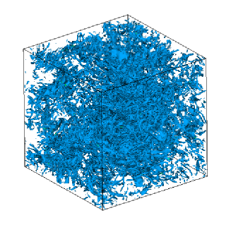
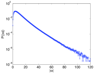
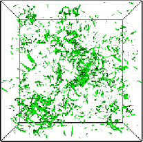
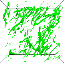
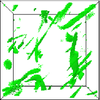
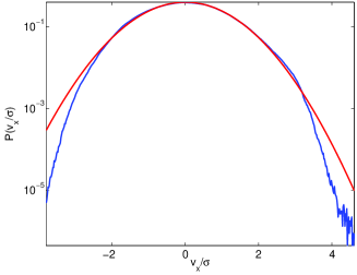
We give illustrative results from a direct numerical simulation DNS with $1024^{3}$ that we have carried out. This study uses the stochastic forcing of   [?] and has attained a Taylor microscale Reynolds number $Re_{\lambda}\sim 100$, where $Re_{\lambda}=u_{rms}\lambda/\nu$; $u_{rms}=\sqrt{2E/3}$ is the root-mean-square velocity and the Taylor microscale $\lambda=\sqrt{\sum E(k)/\sum k^{2}E(k)}$. For state-of-the-art simulations with up to $4096^{3}$ collocation points we refer the reader to Ref. [?]. As we had mentioned in Sec. 2, regions of high vorticity are organised into slender tubes. These can be visualised by looking at isosurfaces of $|\omega|$ as shown in the representative plots of Figs 2 and 3. The right panel of Fig. 2 shows the PDF of $|\omega|$; this has a distinctly non-Gaussian tail. The structure of high-$|\omega|$ vorticity tubes shows up especially clearly in the plots of Fig. 3, the second and third panels of which show successively magnified images of the central part of the first panel (for a $4096^{3}$ version see Ref.   [?]).

Figure  2.: (Color online) (Left) Isosurface plot of $|\omega|$ with $|\omega|$ equal to its mean value. (Right) A semilog plot of the PDF of $|\omega|$.

Figure  3.: (Color online) (Left) Isosurface plot of $|\omega|$ with $|\omega|$ equal to one standard deviation more than its mean value. (Center) A magnified version of the central part of the panel on the left. (Right) A magnified version of the central part of the panel in the middle.

Figure  4.: (Color online) (Left) Joint PDF $P(Q^{*},R^{*})$ of $R^{*}=R/\langle s_{ij}s_{ij}\rangle^{3/2}$ and $Q^{*}=Q/\langle s_{ij}s_{ij}\rangle$ calculated from our DNS. The black curve represents the zero-discriminant (or Vieillefosse) line $27R^{2}/4+Q^{3}=0$. The contour levels are logarithmically spaced. (Right) PDF of the $x$-component of the velocity (here $\sigma$ denotes the standard deviation); the parabolic curve is a Gaussian that is drawn for comparison.

Figure  5.: (Color online) (Left) The compensated energy spectrum $k^{5/3}E(k)$ versus $k\eta$, where $\eta$ is the dissipation scale from our DNS (see text). (Right) PDFs of velocity increments that show marked deviation from Gaussian behaviour (innermost curve), especially at small length scales; the outermost PDF is for the velocity increment with the shorter length scale.

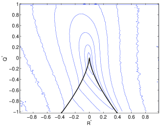
One method to look at these structures is to study the joint PDF of the invariants $Q=-tr(A^{2})/2$ and $R=-tr(A^{3})/3$ of the velocity gradient tensor. The zero-discriminant or Vieillefosse line $D\equiv 27R^{2}/4+Q^{3}=0$ divides the QR plane in different regions. The region with $D>0$ is vorticity dominant (one of the eigenvalues of $A$ is greater than zero whereas the other two eigenvalues are imaginary); the region $D<0$ is strain dominated (all the eigenvalues of $A$ are real). The regions $D>0$ and $D<0$ can be further divided into two more quadrants depending upon the sign of the eigenvalues. In the left panel of Fig. 4 we show a representative contour plot of the joint PDF $P(Q^{*},R^{*})$ obtained from our DNS. The shape of the contour is like a tear-drop, as in experiments   [?], with a tail along the line $D=0$ in the region where $R^{*}>0$ and $Q^{*}<0$. The plot indicates that, in a numerical simulation, most of the structures are vortical but there also exist regions of large strain. For a more detailed discussion of the above classification of different structures we refer the reader to  [?,?].

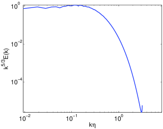
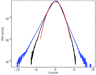
The left panel of Fig. 5 shows a plot of the compensated energy spectrum $k^{5/3}E(k)$ versus $k\eta$ ($\eta$ is the dissipation scale in our DNS). The flat portion at low $k\eta$ indicates agreement with the K41 form $E^{K41}(k)\sim k^{-5/3}$. There is a slight bump after that; this is referred to as a bottleneck (see Ref.   [?] and Sec 6.4); the spectrum then falls in the dissipation range. The right panel of Fig. 5 shows PDFs of velocity increments at different scales $r$. The innermost curve is a Gaussian for comparison; the non-Gaussian deviations increase as $r$ decreases.

We do not provide data for the multiscaling of velocity structure functions in the 3D Navier-Stokes equation. We refer the reader to Ref.  [?] for a recent discussion of such multiscaling. Often the inertial range is quite limited in such studies. This range can be extended somewhat by using the extended-self-similarity (ESS) procedure  [?] in which the slope of a log-log plots of the structure function $S_{p}$ versus $S_{q}$ yields the exponent ratio $\zeta_{p}/\zeta_{q}$; this procedure is especially useful if $q=3$ since $\zeta_{3}=1$ for the 3D Navier-Stokes case. We illustrate the use of this ESS procedure in Sec. (6.3) on 2D turbulence.

The methods of statistical field theory have been used with some success to study the statistical properties of a randomly forced Navier-Stokes equation  [?,?,?,?]. The stochastic force here acts at all length scales; it is Gaussian and has a Fourier-space covariance proportional to $k^{1-y}$. For $y\geq 0$, a simple perturbation theory leads to infrared divergences; these can be controlled by a dynamical renormalization group for sufficiently small $y$; for $y=4$ this yields a K41-type $k^{-5/3}$ spectrum at the one-loop level. This value of $y$ is too large to trust a low-$y$, one-loop result; also, for $y\geq 3$, the sweeping effect leads to another singularity  [?]. Nevertheless, this randomly forced model has played an important role historically. Thus it has been studied numerically via the pseudo-spectral method  [?,?]. These studies have shown that, even though the stochastic forcing destroys the vorticity tubes that we have described above, it yields multiscaling of velocity structure that is consistent, for $y=4$, with the analogous multiscaling in the conventional 3D Navier-Stokes equation, barring logarithmic corrections. We will discuss the analogue of this problem for the stochastically forced Burgers equation in Sec. 6.4.

6.2 Shell Models

Even though shell models are far simpler than their parent partial differential equations (PDEs), they cannot be solved analytically. The multiscaling of equal-time structure functions in such models has been investigated numerically by several groups; an overview of earlier work and details about numerical methods for the stiff shell-model equations can be found in Refs.   [?,?,?]. An illustrative plot of equal-time multiscaling exponents for the GOY shell model is given in the right panel of Fig. 1.

We devote the rest of this Subsection to a discussion of the dynamic multiscaling of time-dependent shell-model structure functions that has been elucidated recently by our group  [?,?,?,?]. So far, detailed numerical studies of such dynamic multiscaling has been possible only in shell models. We concentrate on time-dependent velocity structure functions in the GOY model and their passive-scalar analogues in the advection-diffusion shell model.

In a typical decaying-turbulence experiment or simulation, energy is injected into the system at large length scales (small $k$); it then cascades to small length scales (large $k$); eventually viscous losses set in when the energy reaches the dissipation scale. We will refer to this as cascade completion. Energy spectra and structure functions show power-law forms like their counterparts in statistically steady turbulence. It turns out  [?] that the multiscaling exponents for both equal-time and time-dependent structure functions are universal in so far as they are independent of whether they are measured in decaying turbulence or the forced case in which we get statistically steady turbulence.

Furthermore, the distinction between Eulerian and Lagrangian frameworks assumes special importance in the study of dynamic multiscaling of time-dependent structure functions. Eulerian-velocity structure functions are dominated by the sweeping effect that lies at the heart of Taylor’s frozen-flow hypothesis; this relates spatial and temporal separations linearly (see Sec. 2) whence we obtain trivial dynamic scaling with dynamic exponents $z_{p}^{\cal{E}}=1$ for all $p$, where the superscript $\cal{E}$ stands for Eulerian. By contrast, we expect nontrivial dynamic multiscaling in Lagrangian or quasi-Lagrangian measurements. Such measurements are daunting in both experiments and direct numerical simulations; however, they are possible in shell models. As we have mentioned in Sec. 3, shell models have a quasi-Lagrangian character since they do not have direct sweeping effects. Thus we expect nontrivial dynamic multiscaling of time-dependent structure functions in them.

Indeed, we find that  [?,?,?] that, given a time-dependent structure function, we can extract an infinity of time scales from it. Dynamic scaling Ansätze [cf., Eq. (4)] can then be used to extract dynamic multiscaling exponents. A generalisation of the multifractal model then suggests linear relations, referred to as bridge relations, between these dynamic multiscaling exponents and their equal-time counterparts. These can be related to equal-time exponents via bridge relations. We show how to check these bridge relations in shell models. However, before we present details, we must define time-dependent structure functions precisely.

The order-$p$, time-dependent, structure functions, for longitudinal velocity increments, $\delta u_{\parallel}({\bf x},{\bf r},t)\equiv[{\bf u}({\bf x}+{\bf r},t)-{\bf u}({\bf x},t)]$ and passive-scalar increments, $\delta\theta({\bf x},t,{\bf r})=\theta({\bf x}+{\bf r},t)-\theta({\bf x},t)$ are defined as

$${\mathcal{F}}_{p}^{u}(r,\{t_{1},\ldots,t_{p}\})\equiv\left\langle[\delta u_{\parallel}({\bf x},t_{1},r)\ldots\delta u_{\parallel}({\bf x},t_{p},r)]\right\rangle$$ (62)

and

$${\mathcal{F}}_{p}^{\theta}({\bf r},{t_{1},...,t_{p}})=<[\delta\theta({\bf x},t_{1},{\bf r})...\delta\theta({\bf x},t_{p},{\bf r})]>;$$ (63)

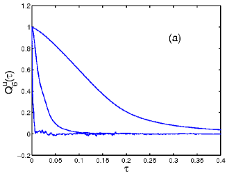
i.e., fluctuations are probed over a length scale $r$ which lies in the inertial range. For simplicity, we consider $t_{1}=t$ and $t_{2}=\ldots=t_{p}=0$ in both Eq. (62) and Eq. (63). Given ${\mathcal{F}}^{u}(r,t)$ and ${\mathcal{F}}^{\theta}(r,t)$, we can define the order-$p$, degree-$M$, integral-time scales and derivative-time scales as follows  [?]:

$${\cal T}^{I,u}_{p,M}(r,t)\equiv\biggl{[}\frac{1}{{\mathcal{S}}^{u}_{p}(r)}\int_{0}^{\infty}{\mathcal{F}}^{u}_{p}(r,t)t^{(M-1)}dt\biggl{]}^{(1/M)};$$ (64)

$${\cal T}^{I,\theta}_{p,M}(r,t)\equiv\biggl{[}\frac{1}{{\mathcal{S}}^{\theta}_{p}(r)}\int_{0}^{\infty}{\mathcal{F}}^{\theta}_{p}(r,t)t^{(M-1)}dt\biggl{]}^{(1/M)};$$ (65)

$${\cal T}^{D,u}_{p,M}(r,t)\equiv\biggl{[}\frac{1}{{\mathcal{S}}^{u}_{p}(r)}\frac{\partial^{M}{\mathcal{F}}^{u}_{p}(r,t)}{\partial t^{M}}\biggl{]}^{(-1/M)};$$ (66)

$${\cal T}^{D,\theta}_{p,M}(r,t)\equiv\biggl{[}\frac{1}{{\mathcal{S}}^{\theta}_{p}(r)}\frac{\partial^{M}{\mathcal{F}}^{\theta}_{p}(r,t)}{\partial t^{M}}\biggl{]}^{(-1/M)}.$$ (67)

Integral-time dynamic multiscaling exponents $z^{I,u}_{p,M}$ for fluid turbulence can be defined via ${\cal T}^{I,u}_{p,M}(r,t)\sim r^{z^{I,u}_{p,M}}$ and the derivative-time ones $z^{D,u}_{p,M}$ by ${\cal T}^{D,u}_{p,M}(r,t)\sim r^{z^{D,u}_{p,M}}$. They satisfy the following bridge relations  [?]:

$$z^{I,u}_{p,M}=1+[\zeta_{p-M}-\zeta_{p}]/M;$$ (68)

$$z^{D,u}_{p,M}=1+[\zeta_{p}-\zeta_{p+M}]/M.$$ (69)

For passive-scalars advected by a turbulent velocity field, the corresponding dynamic multiscaling exponents are defined as ${\cal T}^{I,\theta}_{p,M}(r,t)\propto r^{z^{I,\theta}_{p,M}}$ and ${\cal T}^{D,\theta}_{p,M}(r,t)\propto r^{z^{D,\theta}_{p,M}}$; they satisfy the following bridge relations involving the scaling exponents $\zeta_{M}$ of equal-time, order-$M$ structure functions of the advecting velocity field:

$$z^{I,\theta}_{p,M}=1-\frac{\zeta_{M}}{M},\hskip 28.45274ptz^{D,\theta}_{p,M}=1-\frac{\zeta_{-M}}{M}.$$ (70)

These bridge relations, unlike Eq. (68) and Eq. (69), are independent of $p$. [Recall that, for the Kraichnan model, we have already shown in Sec. 5 that we get simple dynamic scaling.]

GOY-model equal-time structure functions and their associated inertial-range exponents are defined as follows:

$$S^{u}_{p}(k_{n})\equiv\left\langle[u_{n}(t)u^{\ast}_{n}(t)]^{p/2}\right\rangle\sim k_{n}^{-\zeta_{p}}.$$ (71)

The time-dependent structure function are

$$F^{u}_{p}(k_{n},t_{0},t)\equiv\left\langle[u_{n}(t_{0})u^{\ast}_{n}(t_{0}+t)]^{p/2}\right\rangle.$$ (72)

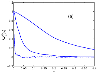
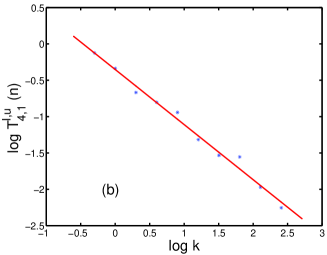
We evaluate these numerically for the GOY shell model [numerical details may be found in Refs.  [?,?]], extract integral and derivative time scales from them and thence the exponents $z^{I,u}_{p,1}$ and $z^{D,u}_{p,2}$, respectively, from slopes of log-log plots of $T^{I,u}_{p,1}(n)$ versus $k_{n}$ (right panel of Fig. 6) and of $T^{D,u}_{p,2}(n)$ versus $k_{n}$ (right panel of Fig. 7).

,

Figure  6.: (Color online) (a) A representative plot of the normalised fourth order time-dependent structure function versus the dimensionless time $\tau$ obtained from the GOY shell model. The plots are for shells 4, 6, and 8 (from top to bottom). (b) A log-log plot of $T^{I,u}_{4,1}(n)$ versus $k$ (for convenience, we have dropped the subscript $n$ in the label of the x-axis in the figure); a linear fit gives the dynamic mulstiscaling exponent $z^{I,u}_{4,1}$.

,

Figure  7.: (Color online) (a) A representative plot of the normalised sixth order time-dependent structure function versus the dimensionless time $\tau$ obtained from the GOY shell model. The plots are for shells 4, 6, and 8 (from top to bottom). (b) A log-log plot of $T^{D,u}_{6,2}(n)$ versus $k$ (for convenience, we have dropped the subscript $n$ in the label of the x-axis in the figure); a linear fit gives the dynamic multiscaling exponent $z^{D,u}_{6,2}$.

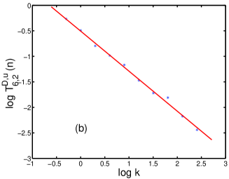
There is excellent agreement (within error bars) of the multiscaling exponents $z^{I,u}_{p,1}$ and $z^{D,u}_{p,2}$, obtained from our simulations, with the values computed from the appropriate bridge relations using the equal-time exponents, $\zeta_{p}$.

For the passive-scalar case, the equal-time order-$p$ structure functions is

$$S^{\theta}_{p}(k_{n})\equiv\left\langle[\theta(t)\theta^{\ast}_{n}(t)]^{p/2}\right\rangle\sim k_{n}^{-\zeta^{\theta}_{p}}$$ (73)

and its time-dependent version is

$$F^{\theta}_{p}(k_{n},t_{0},t)=<[\theta_{n}(t_{0})\theta_{n}^{*}(t_{0}+t)]^{p/2}>.$$ (74)

We consider decaying turbulence here with $t_{0}$ a time origin. It is useful now to work with the normalised time-dependent structure function, $Q^{\theta}_{p}(n,t_{0},t)=\frac{F^{\theta}_{p}(k_{n},t_{0},t)}{F^{\theta}_{p}(k_{n},t,0)}$. For the case of passive-scalars advected by a velocity field which is turbulent (a solution of the GOY model), we calculate the integral (for $M$ = $1$) and derivative time scales (for $M$ = $2$) corresponding to Eq.(58) and Eq.(60), respectively. The slope of a log-log plot of $T^{I,\theta}_{p,1}(n)$ vs $k_{n}$ yields the integral time scale exponent, $z^{I,\theta}_{p,1}$, since $T^{I,\theta}_{p,1}(n)\propto k_{n}^{-z^{I,\theta}_{p,1}}$. Likewise, from plots of the derivative time scales we extract the exponent $z^{D,\theta}_{p,2}$. For a detailed discussion on dynamic multiscaling in this model we refer the reader to Refs.  [?,?].

6.3 2D Navier-Stokes Turbulence

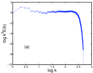
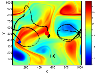
We now consider illustrative numerical calculations for the 2D NS equations (9)-(11). We begin with periodic boundary conditions for which we can use a pseudo-spectral method similar to the one given in the previous Subsection for the 3D NS case. We study decaying turbulence first with the source function $f$ (the ${\hat{\bf z}}$ component of the curl of some force ${\nabla\times\bf F}$) set to 0. We use $1024^{2}$ collocation points and the standard $2/3$ dealiasing procedure; for time marching we use a second-order Runge-Kutta scheme  [?]. Our initial condition $|\omega(k)|^{2}=k^{-3}\exp(-k^{2})$ leads to a forward cascade. We seed the flow with Lagrangian tracers and use a cubic spline interpolation method to calculate their trajectories   [?]. Representative plots from our from our DNS are shown in Fig. 8. The first part (Fig. 8a) shows a compensated energy spectrum $k^{3}E(k)$ for the case with no Ekman friction. Figure 8b, from a DNS with Ekman friction $\alpha_{E}=0.1$, Kolmogorov forcing  [?], and periodic boundary conditions, shows a trajectory of a Lagrangian tracer superimposed on a pseudocolour plot of the vorticity field at time $t=100$; the tracer starts at the point marked with a circle ($t=0$) and ends at the star ($t=100$). For a state-of-the-art simulation that resolves both forward and inverse cascades in a forced DNS of 2D turbulence we refer the reader to Ref.  [?]; such DNS studies have also investigated the scaling properties of structure functions and have provided some evidence for conformal invariance in the inverse cascade inertial range  [?].

,

Figure  8.: (Color online) (a) A log-log plot of the compensated energy spectrum $k^{3}E(k)$ versus $k$ from our DNS, of resolution $1024^{2}$, of two dimensional decaying turbulence with periodic boundary conditions. The flat region indicates a scaling form $E(k)\sim k^{-3}$. (b) The trajectory of a single Lagrangian particle over a time of order 100 in a two-dimensional flow with drag and forcing. The starting point of the trajectory is in the middle of the box and is indicated by a red circle; the end point is indicated by a blue star. The trajectory is superimposed on a pseudocolor plot of the vorticity field corresponding to the time at the end of the Lagrangian trajectory. The figure corresponds to a forced DNS of resolution $1024^{2}$ with periodic boundary conditions, statistical steady state, and with a coefficient of Ekman friction $\alpha_{E}=0.1$.

We end with an illustrative example of a recent DNS study  [?] that sheds light on the effect of the Ekman friction on the statistics of the forward cascade in wall-bounded flows that are directly relevant to laboratory soap-film experiments  [?,?,?,?]. The details of this DNS are given in Ref.  [?]. In brief, $\omega$ is driven to a statistical steady state by a deterministic Kolmogorov forcing $F_{\omega}\equiv k_{inj}F_{0}\cos(k_{inj}x)$, with $F_{0}$ the amplitude and $k_{inj}$ the wavenumber on which the force acts; no-slip and no-penetration boundary conditions are imposed on the walls. The important non-dimensional control parameters are the Grashof number ${\mathcal{G}}=2\pi||F_{\omega}||_{2}/(k_{inj}^{3}\rho\nu^{2})$ and the non-dimensional Ekman friction $\gamma=\alpha_{E}/(k_{inj}^{2}\nu)$, where we non-dimensionalize $F_{\omega}$ by $2\pi/(k_{inj}||F_{\omega}||_{2})$, with $||F_{\omega}||_{2}\equiv(\int_{A}|F_{\omega}|^{2}d{\bf x})^{1/2}$ and the length and time scales are made non-dimensional by scaling ${\bf x}$ by $k_{inj}^{-1}$ and $t$ by $k_{inj}^{-2}/\nu$. We use a fourth-order Runge-Kutta scheme for time marching and evaluate spatial derivatives via second-order and fourth-order, centered, finite differences, respectively, for points adjacent to the walls and for points inside the domain. The Poisson equation is solved by using a fast-Poisson solver  [?] and $\omega$ is calculated at the boundaries by using Thom’s formula  [?].

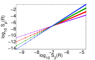
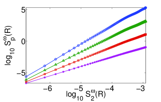
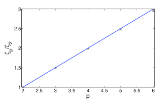
Since Kolmogorov forcing is inhomogeneous, we use the decomposition $\psi=\langle\psi\rangle+\psi^{\prime}$ and $\omega=\langle\omega\rangle+\omega^{\prime}$, where the angular brackets denote a time average and the prime the fluctuating part to calculate the order-$p$ velocity and vorticity structure functions. Since this is a wall-bounded flow, it is important to extract the isotropic parts of these structure functions  [?,?]. Furthermore, given our resolution ($2049^{2}$), it becomes necessary to use the ESS procedure to extract exponent ratios. Illustrative log-log ESS plots for velocity, $S_{p}(R)$, and vorticity, $S^{\omega}_{p}(R)$, structure functions are shown in the left and right panels, respectively, of Fig. 9; their slopes yield the exponent ratios that are plotted versus the order $p$ in Fig. 10. The Kraichnan-Leith-Batchelor (KLB) predictions  [?] for these exponent ratios, namely, $\zeta^{KLB}_{p}/\zeta^{KLB}_{2}\sim r^{p/2}$ and $\zeta_{p}^{\omega,KLB}/\zeta_{2}^{\omega,KLB}\sim r^{0}$, agree with our values for $\zeta_{p}/\zeta_{2}$ but not $\zeta_{p}^{\omega}/\zeta_{2}^{\omega}$: velocity structure functions do not display multiscaling [left panel of Fig. 10] whereas their vorticity analogs do [note the curvature of the plot in the right panel of Fig. 10]. Similar results have been seen in DNS studies with periodic boundary conditions  [?,?]. Additional results for PDFs of several properties can be obtained from our DNS  [?]; these are in striking agreement with experimental results  [?].

Figure  9.: (Color online) (Left) Log-log ESS plots of the isotropic parts of the order-$p$ velocity structure functions $S_{p}(R)$ versus $S_{2}(R)$; $p=3$ (purple line with dots), $p=4$ (red line with square), $p=5$ (green line with triangles), and $p=6$ (blue line with circles). According to the KLB prediction $S_{p}(R)\sim R^{\zeta}_{p}$. (Right) Log-log ESS plots of the isotropic parts of the order-$p$ vorticity structure functions $S_{p}(R)$ versus $S_{2}(R)$; $p=3$ (purple line with stars), $p=4$ (red line with square), $p=5$ (green line with triangles), and $p=6$ (blue line with circles).

Figure  10.: (Color online) (Left) Plots of the exponent ratios $\zeta_{p}/\zeta_{2}$ versus $p$ for the velocity differences. (Right) Plots of the exponent ratios $\zeta^{\omega}_{p}/\zeta^{\omega}_{2}$ versus $p$ for the vorticity differences.

6.4 The One dimensional Burgers Equation

In this Subsection we present a few representative numerical studies of the 1D Burgers equation. The first of these uses a pseudo-spectral method with $2^{14}$ collocation points, the $2/3$ dealising rule, and a fourth-order Runge-Kutta time-marching scheme. In the second study of a stochastically forced Burgers equation (see below) we use a fast-Legendre method that yields results in the zero-viscosity limit  [?].

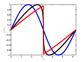
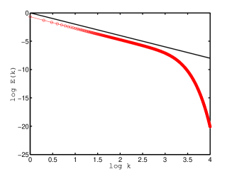
For the Burgers equation with no external forcing and sufficiently well-behaved initial conditions, the velocity field develops shocks, or jump discontinuities, which merge into each other with time. The time at which the first shock appears is usually denoted by $t_{*}$. For all times greater than $t_{*}$, it is possible to calculate, analytically, the scaling exponents $\zeta_{p}$ for the equal-time structure functions via $S_{p}\equiv\langle[u(x+r,t)-u(x)]^{p}\rangle\sim C_{p}|r|^{p}+C_{p}^{\prime}|r|$, where the first term comes from the ramp, and the second term comes from the probability of having a shock in the interval $|r|$. As a consequence of this we have bifractal scaling : for $0<p<1$ the first term dominates leading to $\zeta_{p}=p$ and for $p>1$ the second one dominates giving $\zeta_{p}=1$. This leads to an energy spectrum $E(k)\sim k^{-2}$. Representative plots from our pseudo-spectral DNS, with $\nu=10^{-3}$ and an initial condition $u(x)=$sin($x$) (for which $t_{*}=1$) are shown in Fig. 11; the left panel shows plots of the velocity field at times $t=0,\,1,$ and $t=1.5$ and the right panel the energy spectrum at $t=1$.

,

Figure  11.: (Color online) (Left) Snapshots of the solution of the Burgers equation obtained from our DNS with initial condition $u(x)=$sin $x$ at times $t=0$ (blue), $t=1$ (black) and $t=2$ (red). (Right) A representative log-log plot of $E(k)$ versus $k$, at time $t=1$ for the Burgers equation with initial conditions $u(x)=$ sin $x$.

The stochastically forced Burgers equation has played an important role in renormalization-group studies  [?]. In particular, consider a Gaussian random force $f(x,t)$ with zero mean and the following covariance in Fourier space:

$$\langle{\hat{f}}(k_{1},t_{1}){\hat{f}}(k_{2},t_{2})\rangle=2D_{0}|k|^{\beta}\delta(t_{1}-t_{2})\delta(k_{1}+k_{2});$$ (75)

here ${\hat{f}}(k,t)$ is the spatial Fourier transform of $f(x,t)$, $D_{0}$ is a constant, and the scaling properties of the forcing is governed by the exponent $\beta$. For positive values of $\beta$, the Burgers equation can be studied by using renormalization-group techniques; specifically, for $\beta=2$ one recovers simple (Kardar-Parisi-Zhang or KPZ) scaling with the equal-time exponent $\zeta_{p}=p$. It was hoped that forcing with negative values of $\beta$ (in particular $\beta=-1$), which cannot be studied by renormalization-group methods, might yield multiscaling of velocity structure functions.

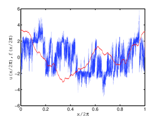
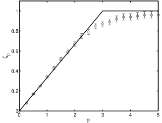
However, our high-resolution study  [?], which uses a fast-Legendre method, has shown that the apparent multiscaling of structure functions in this stochastic model might arise because of numerical artifacts. The general consensus is that this stochastically forced Burgers model should show bifractal scaling. In Fig. 12 we present representative plots of the velocity field (left panel, blue curve) and the scaling exponents (right panel) for this model. We have obtained the data for these figures by using a fast-Legendre method with $2^{18}$ collocation points.

,

Figure  12.: (Color online) (Left) A snapshot of the velocity field (jagged line in blue) in steady state and the force in red from our fast-Legendre method DNS of the stochastically forced Burgers equation. (Right) A representative plot of the exponents $\zeta_{p}$, with error-bars, for the equal-time velocity structure functions of the stochastically forced Burgers equation; bifractal scaling is shown by the black solid line; the deviations from this are believed to arise from artefacts (see text).

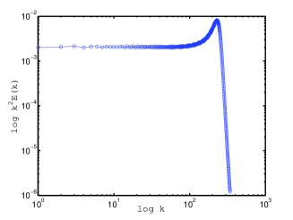
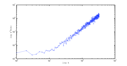
Numerical studies of the Burgers equation have also proved useful in elucidating bottleneck structures in energy spectra   [?,?](cf., the spectrum in the left panel of Fig. 5). It turns out that such a bottleneck does not occur in the conventional Burgers equation. However, it does  [?] occur in the hyperviscous one, in which usual Laplacian dissipation operator is replaced by its $\alpha^{\rm th}$ power; this is known as hyperviscosity for $\alpha>1$. We show a representative compensated energy spectrum for the case $\alpha=4$ in the left panel of Fig. 13. We have obtained this from a pseudo-spectral DNS with $2^{12}$ collocation points. The $\alpha\to\infty$ limit is very interesting too since, in this limit, the hyperviscous Burgers equation maps on to the Galerkin-truncated version of the inviscid Burgers equation. In this Galerkin-truncated inviscid case, the Fourier modes thermalise   [?,?]; in a compensated energy spectrum this shows up as $E(k)\sim k^{2}$, for large $k$ [see the right panel of Fig. 13 for the case $\alpha=200$]. Such thermalisation effects in the Galerkin-truncated Euler equation have also attracted a lot of attention  [?]; and the link between bottlenecks and thermalisation has been explored in our recent work  [?] to which we refer the interested reader.

,

Figure  13.: (Color online) (Left) A representative log-log plot of a bottleneck in the compensated energy spectrum $k^{2}E(k)$ of a hyperviscous Burgers equation with $\alpha=4$. (Right) A representative log-log plot of $k^{2}E(k)$ versus $k$ for $\alpha=200$ at time $t=30$. We see clear signatures of thermalization at large $k$ (see text).

6.5 Turbulence with Polymer Additives

In this Subsection, we present a few results from our numerical study  [?] of the analogue drag reduction by polymer additives in homogeneous, isotropic turbulence. This requires a DNS of considerably greater complexity than the ones we have described above. A naïve pseudospectral method cannot be used for the FENE-P model given in Eqs. (18) and (19): the polymer conformation tensor $\cal{C}$ is symmetric and positive definite; however, in a practical implementation of the pseudo-spectral method it loses this property. We have employed a numerical technique that uses a Cholesky decomposition to overcome this problem; we refer the reader to Ref.  [?] for these details.

Our recent DNS of this model has shown that the natural analogue drag reduction in decaying, homogeneous, isotropic turbulence is dissipation reduction; the percentage reduction DR can be defined as

$${\rm DR}\equiv\left(\frac{\epsilon^{f,m}-\epsilon^{p,m}}{\epsilon^{f,m}}\right)\times 100;$$ (76)

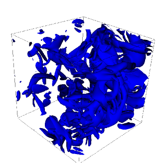
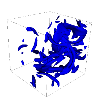
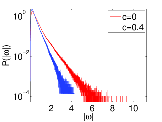
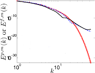
here the superscripts $f$ and $p$ stand, respectively, for the fluid without and with polymers and the superscript $m$ indicates the time $t_{m}$ at which the cascade is completed. The dependence of DR on the polymer concentration parameter $c$ and the Weissenberg number may be found in Ref.  [?]. Here we show how the addition of polymers reduces small-scale structures in the turbulent flow: By a comparison of the isosurfaces of $|\omega|$ in the left (without polymers) and right (with polymers) panels of Fig. 14, we see that slender vorticity filaments are suppressed by the polymers; this is in qualitative agreement with experiments  [?]. The PDFs of $|\omega|$, with and without polymers (left panel of Fig. 15) confirm that regions of large vorticity are reduced by polymers. The right panel of Fig. 15 shows how the polymers modify the energy spectrum in the dissipation range; this behaviour has been seen in recent experiments  [?], which study the second-order structure function that is related simply to the energy spectrum. For a full discussion of these and related results we refer the reader to Ref.  [?,?].

,

Figure  14.: (Color online) Constant-$|\omega|$ isosurfaces for $|\omega|=\langle{|\omega|}\rangle+\sigma$ at cascade completion without and (Right) with polymers ($c=0.4$); $\langle|\omega|\rangle$ is the mean and $\sigma$ the standard deviation of $|\omega|$.

,

Figure  15.: (Color online) (Left) PDF of $\omega$ at cascade completion without ($c=0$) and with polymers ($c=0.4$). Note that regions of large vorticity are reduced on the addition of polymers. (Right) Representative plots of the energy spectra $E^{p,m}(k)$ or $E^{f,m}(k)$ versus $k$ for $c=0.1$ (blue dashed line) and $c=0.4$ (solid line).

7. Conclusions

Turbulence provides us with a variety of challenging problems. We have tried to give an overview of some of these, especially those that deal with the statistical properties of turbulence. The choice of topics has been influenced, of course, by the areas in which we have carried out research. For complementary, recent overviews we refer the reader to Refs.  [?,?,?]; we hope the other reviews and books that we have cited to will provide the reader with further details.

We would like to thank CSIR, DST, and UGC (India) for support, and SERC (IISc) for computational resources.

REFERENCES

- [1] R. Ecke, Los Alamos Science, 29, 124 (2005).
- [2] G. Falkovich and K.R. Sreenivasan, Physics Today 59, 43 (2006).
- [3] I. Procaccia and K.R. Sreenivasan, Physica D 237, 2167 (2008) and references therein.
- [4] A.J. Reynolds Turbulent flows in engineering (John Wiley, New York, 1974).
- [5] S.B. Pope, Turbulent Flows (Cambridge University, Cambridge, UK, 2000).
- [6] C. Doering, Annu. Rev. Fluid Mech., 41, 109 (2009).
- [7] C. Fefferman, Existence and smoothness of the Navier-Stokes equation. Clay Millenium Prize Problem Description (2000); http://www.claymath.org/millennium/Navier-Stokes_Equations/Official_Problem_D escription.pdf.
- [8] P. Constantin and C. Foias, Navier-Stokes Equations (University of Chicago Press, Chicago, 1988).
- [9] C. Doering and J. Gibbon, Applied Analysis of the Navier-Stokes Equations (Cambridge University Press, Cambridge, UK, 1995).
- [10] A.J. Majda and A.L. Bertozzi, Vorticity and Incompressible Flow (Cambridge University Press, Cambridge, UK, 2001).
- [11] H. Tennekes and J. L. Lumley, A First Course in Turbulence (MIT Press, Cambridge, Massachusetts, 1972).
- [12] M. Lesieur, Turbulence in Fluids (Springer, The Netherlands, 2008).
- [13] P.A. Davidson, Turbulence: An Introduction for Scientists and Engineers (Oxford University Press, Oxford, 2007).
- [14] V.M. Canuto and J. Christensen-Dalsgaard, Annu. Rev. Fluid Mech. 30, 167 (1998); Turbulence and Magnetic Fields in Astrophysics, eds. E. Falgarone and T. Passot, (Springer, New York, 2003); M.S. Miesch and J. Toomre Annu. Rev. Fluid Mech. 41, 317 (2009).
- [15] A. Rai Choudhuri, The Physics of Fluids and Plasmas: An Introduction for Astrophysicists (Cambridge University Press, Cambridge, UK, 1998).
- [16] V. Krishan, Astrophysical Plasmas and Fluids (Kluwer, Dordrecht, (1999).
- [17] H. Goedbloed and S. Poedts, Principles of Magnetohydrodynamics With Applications to Laboratory and Astrophysical Plasmas (Cambridge University Press, Cambridge, UK, 2004).
- [18] A S Monin, Russ. Math. Surv. 38 127 (1983); P. Bradshaw and J. D. Woods, in Turbulence, ed. P. Bradshaw, (Springer, New York, 1978); A.J. Majda and X. Wang, Nonlinear Dynamics and Statistical Theories of Basic Geophysical Flows (Cambridge University Press, Cambridge, UK, 2006).
- [19] G. Boer and T. Shepherd, J. Atmos. Sci. 40, 164 (1983).
- [20] R.A. Shaw, Annu. Rev. Fluid Mech., 35, 183 (2003).
- [21] D. Biskamp, Magnetohydrodynamic Turbulence (Cambridge University Press, Cambridge, UK, 2003).
- [22] M.K. Verma, Phys. Rep. 401, 229 (2004).
- [23] S. Orszag, in Fluid Dynamics, Les Houches, eds. R. Balian and J. Peube (Gordon and Breach, New York, 1977) pp. 237-374.
- [24] H. Rose and P. Sulem, J. Phys. France 39, 441 (1978).
- [25] C.D. Dominicis and P. Martin, Phys. Rev. A 19, 419 (1979).
- [26] V. Yakhot and S. Orszag, Phys. Rev. Lett 57, 1722 (1986).
- [27] W.D. McComb, The Physics of Fluid Turbulence, (Oxford University Press, Oxford, 1991).
- [28] G.L. Eyink, Phys. Fluids A. 6 3063 (1994); G.L. Eyink and N. Goldenfeld, Phys. Rev. E 50 4679 (1994).
- [29] T. Bohr, M.H. Jensen, G. Paladin, and A. Vulpiani, Dynamical Systems Approach to Turbulence (Cambridge University, Cambridge, UK, 1998).
- [30] L. Ts. Adzhemyan, N.V. Antonov, and A.N. Vasiliev, The Field Theoretic Renormalization Group in Fully Developed Turbulence (Gordon and Breach, 1999).
- [31] J.K. Bhattacharjee and S. Bhattacharyya, Nonlinear Dynamics Near and Far From Equilibrium (Hindustan Book Agency, New Delhi, 2007), Ch. 8, pp 231-274.
- [32] Non-equilibrium Statistical Mechanics and Turbulence, eds. S. Nazarenko and O.V. Zaboronski (Cambridge University Press, Cambridge, UK, 2008).
- [33] U. Frisch, Turbulence: The Legacy of A.N. Kolmogorov (Cambridge University, Cambridge, UK, 1996).
- [34] G. Falkovich, K. Gawedzki and M. Vergassola, Rev. Mod. Phys. 73, 913 (2001).
- [35] P. Tabeling, Phys. Rep. 362, 1 (2002).
- [36] H. Kellay and W. Goldburg, Rep. Prog. Phys. 65 845 (2002).
- [37] J.M. Burgers, The Nonlinear Diffusion Equation, (D. Reidel, Dordrecht, 1974).
- [38] U. Frisch and J. Bec, Les Houches 2000: New Trends in Turbulence, ed. M. Lesieur, (Springer EDP-Sciences 2000)
- [39] J. Bec and K. Khanin, Phys. Rep., 447, 1 (2007).
- [40] J. Lumley, J. Polym. Sci. 7, 263 (1973).
- [41] I. Procaccia, V. S. L’vov, and R. Benzi, Rev. Mod. Phys., 80, 225 (2008).
- [42] C.M. White and M.G. Mungal, Annu. Rev. Fluid Mech., 40, 235 (2008).
- [43] G.K. Batchelor The Theory of Homogeneous Turbulence (Cambridge University, Cambridge, UK, 1953).
- [44] A.S. Monin and A.M. Yaglom, Statistical Fluid Mechanics, Vols. 1 and 2 (Dover, New York, 2007).
- [45] R. Pandit, S.S. Ray, and D. Mitra, Eur. Phys. J. B 64, 463 (2008).
- [46] S.S. Ray, D. Mitra, and R. Pandit, New J. Phys. 10, 033003 (2008).
- [47] G. Ahlers, S. Grossmann, and D. Lohse, Rev. Mod. Phys. 81, 503-538 (2009) and references therein.
- [48] J. Tough, in Progress in Low Temperature Physics, ed. D. F. Brewer (North-Holland, Amsterdam, 1982), Vol. VIII, p. 133.
- [49] See, e.g., M. Cencini, J. Bec, L. Biferale, G. Boffetta, A. Celani, A. Lanotte, S. Musacchio and F. Toschi, J. Turb. 7, 1 (2006).
- [50] P.G. Drazin and W.H. Reid, Hydrodynamic Stability Second Edition (Cambridge University Press, Cambridge, UK, 2004).
- [51] J. Moehlis, H. Faisst, and B. Eckhardt, New J. Phys. 6, 56 (2004).
- [52] H. Schlichting and K. Gersten, Boundary Layer Theory (Springer, New Delhi, 2006).
- [53] H.M. Nagib, K.A. Chauhan, and P. Monkewitz, Phil. Trans. R. Soc. A, 365, 755 (2007).
- [54] See, e.g.: G.I. Barenblatt and A.J. Chorin, Phys. Fluids, 10, 1043 (1998); S. Hoyas and J. Jimenez, Phys. Fluids, 18, 011702 (2006); B.J. McKeon, J. Li, W. Jiang, J.F. Morrison and A.J. Smits, J. Fluid Mech. 501, 135 (2004); A.J. Smits and M.V. Zagarola, Phy. Fluids, 10, 1045 (1998); R.L. Panton, Phil. Trans. R. Soc. A 365, 733 (2007); V. L’vov, I. Procaccia, and O. Rudenko Phys. Rev. Lett. 100, 054504 (2008) and references therein.
- [55] L.F. Richardson Weather Prediction by Numerical Process (Cambridge Univ. Press, 1922).
- [56] A.N. Kolmogorov, Dokl. Akad. Nauk SSSR 30, 301 (1941); A.N. Kolmogorov, Dokl. Akad. Nauk SSSR 31, 538 (1941).
- [57] T. Kurian and J.H.M. Fransson, Fluid Dyn. Res. 41, 021403 (2007).
- [58] N. Mordant, P. Metz, O. Michel, and J-F Pinton Phys. Rev. Lett. 87, 214501 (2001); N. Mordant, E. Lévque, and J-F Pinton, New J. Phys. 6, 116 (2004).
- [59] A. La Porta, G.A. Voth, A.M. Crawford, J. Alexander, E. Bodenschatz Nature 409, 1017 (2001); G.A. Voth, A. La Porta, A.M. Crawford, J. Alexander, and E. Bodenschatz J. Fluid Mech. 469, 121 (2002); A.M. Reynolds, N. Mordant, A.M. Crawford and E Bodenschatz, New J. of Phys. 7, 58 (2005); F. Toschi and E. Bodenschatz, Annu. Rev. Fluid Mech., 41, 375 (2009).
- [60] A. Arneòdo, et al., Phys. Rev. Lett. 100, 254504 (2008).
- [61] G.J. Kunkel and I. Marusic, J. Fluid Mech. 548, 375 (2006).
- [62] E.L. Andreas, K.J. Claffey, R.E. Jordan, C.W. Fairall, P.S. Guest, P.O.G. Persson, and A.A. Grachev, J. Fluid Mech. 559, 117 (2006).
- [63] G. Gulitski, M. Kholmyansky, W. Kinzelbach, B. Lüthi, A. Tsinober and S. Yorish, J. Fluid Mech., 589, 57 (2007); ibid, 83 (2007); ibid 103 (2007).
- [64] A. Talamelli, F. Persiani, J.H.M. Fransson, P.H. Alfredsson, A.V. Johansson, H.M. Nagib, J-D Rüedi, K.R. Sreenivasan, and P.A. Monkewitz, Fluid Dyn. Res. 41, 021407 (2009).
- [65] H.L. Grant, R.W. Stewart, and A. Moilliet, J. Fluid Mech. 12, 241 (1968); Marine turbulence: theories, observations, and models H.Z. Baumert, J.H. Simpson, and J. Sündermann (Cambridge University Press, Cambridge, UK 2005).
- [66] S. Tavoularis, Measurement in Fluid Mechanics (Cambridge University Press, Cambridge, UK, 2005).
- [67] See, e.g., B.J. Mckeon, G. Comte-Bellot, J.F. Foss, J. Westereeel, F. Scarano, C. Tropea, J.F. Meyers, J.W. Lee, A.A. Cavone, R. Schodl, M.M. Kochesfahani, D.G. Nocera, Y. Andreopoulos, W.J.A. Dahm, J.A. Mullin, J.M. Wallace, P.V. Vukoslavcevic, S.C. Morris, E.R. Pardyjak, and A. Cuerva, in Springer Handbook of Experimental Fluid Mechanics, eds. C. Tropea, A.L. Yarin, and J.F. Foss (Springer, Berlin 2007) pp 215-471.
- [68] See, e.g., P.V. Vukoslavcević, N. Beratlis, E. Balaras, J.M. Wallace, and O. Sun, Exp. Fluids, 46, 109 (2009).
- [69] See, e.g., G.E. Elsinga, F. Scarano, B. Wieneke, and B.W. van Oudheusden, Exp. Fluids, 41, 933 (2006).
- [70] See, e.g., B. Tao, J. Katz, and C. Meneveau, Phys. Fluids, 12, 941 (2000).
- [71] See, e.g., J. Sheng, E. Malkiel, and J. Katz, Exp. Fluids, 45, 1023 (2008).
- [72] M. Van Dyke, An Album of Fluid Motion (The Parabolic Press, Stanford, California, 1988); see also the Gallery of Fluid Motion http://pof.aip.org/pof/gallery/index1.jsp.
- [73] G.L. Brown, A. Roshko, J. Fluid Mech. 64, 775 (1974).
- [74] R.H. Kraichnan and D. Montgomery, Rep. Prog. Phys. 43, 547 (1980).
- [75] R. Kraichnan, Phys. Fluids 10, 1417 (1967); C. Leith, Phys. Fluids, 11, 671 (1968); G. Batchelor, Phys. Fluids Suppl. II 12, 233 (1969).
- [76] S. Douady, Y. Couder, and M.E. Brachet, Phys. Rev. Lett. 67, 983 (1991).
- [77] H. Mouri and A. Hori, Fluid Dyn. Res. 41, 021402 (2009).
- [78] C. Meneveau and K.R. Sreenivasan, J. Fluid Mech. 224, 429 (1991).
- [79] T. Isihara, T. Gotoh, and Y. Kaneda, Annu. Rev. Fluid Mech., 41, 165 (2009).
- [80] C. Kalelkar, Phys.Rev. E 72, 056307 (2005).
- [81] F. Anselmet, Y. Gagne, E. Hopfinnger, and R. Antonia, J. Fluid Mech. 140, 63 (1984).
- [82] Z-S. She and E. Leveque Phys. Rev. Lett. 72, 336 (1994).
- [83] K.R. Sreenivasan and R.A. Antonia, Annu. Rev. Fluid Mech. 29, 435 (1997).
- [84] A. Praskovsky and S. Oncley, Phys. Rev. Lett. 73, 3399 (1994).
- [85] J. Sommeria, J. Fluid Mech. 170, 139 (1986).
- [86] Y. Couder, J. Physique Lett. 45, 353 (1984).
- [87] M. Rivera and X.L. Wu, Phy. Rev. Lett. 85, 976 (2000); M. Rivera, X.L. Wu, and C. Yeung, Phys. Rev. Lett. 87, 044501 (2001); W.B. Daniel and M.A. Rutgers, Phys. Rev. Lett. 89, 134502 (2002); M. Rivera and R. Ecke, arXiv:0710.5888v1 (2007).
- [88] J. Chomaz, J. Fluid Mech. 442, 387 (2001).
- [89] P. Perlekar and R. Pandit, to be published (see http://arxiv.org/abs/0811.1324).
- [90] A. Groisman and V. Steinberg, New J. Phys. 6, 29 (2004).
- [91] S. Berti, A. Bistagnino, G. Boffetta, A. Celani, and S. Musacchio Phys. Rev. E 77, 055306(R) (2008).
- [92] B.A. Toms, in Proc. Intl. Rheological Congress Holland, 1948, p. 135 (1949).
- [93] J.W. Hoyt, Trans. ASME:J. Basic Engng 94, 258 (1972).
- [94] P.S. Virk, AIChE J. 21, 625 (1975).
- [95] K.R. Sreenivasan and C.M. White, J. Fluid Mech., 409, 149 (2000).
- [96] N.T. Ouellette, H. Xu, and E. Bodenschatz, to be published (2009); see arXiv:0708.3945.
- [97] R. Kraichnan, Phys. Fluids 11, 945 (1968); R. Kraichnan, Phys. Rev. Lett. 72, 1016 (1994); R. Kraichnan, Phys. Rev. Lett. 78, 4922 (1997).
- [98] T. Vaithianathan and L. Collins, J. Comput. Phys. 187, 1 (2003).
- [99] E. Gledzer, Sov. Phys. Dokl. 18, 216 (1973); K. Ohkitani and M. Yamada, Prog. Theor. Phys. 81, 329 (1989).
- [100] A. Wirth and L. Biferale, Phys. Rev. E 54, 4982 (1996); M.H. Jensen, G. Paladin, and A. Vulpiani, Phys. Rev. A 45, 7214 (1992).
- [101] C. Kalelkar, R. Govindarajan, and R. Pandit, Phys. Rev. E 72, 017301 (2005).
- [102] V.I. Belinicher and V.S. L’vov, Sov. Phys. JETP 66, 303(1987).
- [103] V.S. L’vov, E. Podivilov, and I. Procaccia, Phys. Rev. E 55, 7030 (1997).
- [104] A. M. Obukhov, Izv. Akad. SSSR, Serv. Geogr. Geofiz. 13, 58 (1949).
- [105] S. Corrsin, J. Appl. Phys. 22, 469 (1951).
- [106] D. Stauffer, M. Ferer, and M. Wortis 29, 345 (1972); A. Aharony, Phys. Rev. B, 9, 2107 (1974).
- [107] G. Parisi and U. Frisch in Turbulence and Predictability of Geophysical Fluid Dynamics, eds. M. Ghil, R. Benzi, and G. Parisi (North-Holland, Amsterdam, 1985) p 84.
- [108] G. Boffetta, A. Mazzino, and A. Vulpiani, J. Phys. A: Math. Gen. 41, 363001 (2008).
- [109] D. Mitra and R. Pandit, Phys. Rev. Lett. 93, 024501 (2004).
- [110] D. Mitra and R. Pandit, Phys. Rev. Lett. 95, 144501 (2005).
- [111] A. Vincent and M. Meneguzzi, J. Fluid Mech. 225, 1 (1991).
- [112] C. Canuto, M. Hussaini, A. Quarteroni, and T. Zang, Spectral Methods in Fluid Dynamics (Spinger-Verlag, Berlin, 1988).
- [113] W. Press, B. Flannery, S. Teukolsky, and W. Vetterling, pp. 848-852, Numerical Recipes in Fortran (Cambridge University Press, Cambridge, 1992).
- [114] V. Eswaran and S. Pope, Comput. Fluids, 16, 257 (1988); the forcing is stochastic and is generated by an Ornstein-Uhlenbeck process (i.e., the noise is coloured).
- [115] B. J. Cantwell, Phys Fluids A 4, 782 (1992).
- [116] Y. Kaneda et al., Phys. Fluids 15, L21 (2003).
- [117] R. Benzi et al., Phys. Rev. E 48, R29 (1993); S. Dhar, A. Sain, and R. Pandit, Phys. Rev. Lett. 78, 2964 (1997).
- [118] C. Y. Mou and P. B. Weichman, Phys. Rev. Lett. 70, 1101 (1993).
- [119] A. Sain, Manu, and R. Pandit, Phys. Rev. Lett. 81, 4377 (1998).
- [120] L Biferale, M Cencini, A S Lanotte, M Sbragaglia and F Toschi, New J. Phy. 637 (2004).
- [121] L. Biferale, Annu. Rev. Fluid Mech., 35, 441 (2003).
- [122] P.K. Yeung, Annu. Rev. Fluid Mech., 34, 115 (2002).
- [123] G. Boffetta, J. Fluid Mech. 589, 253 (2007).
- [124] D. Bernard, G. Boffetta, A. Celani, and G. Falkovich, Nature Physics 2 124 (2006); D. Bernard, G. Boffetta, A. Celani, and G. Falkovich, Phys. Rev. Lett. 98 024501 (2007).
- [125] M. Rivera and X.L. Wu, Phy. Rev. Lett. 85, 976 (2000).
- [126] M. Rivera, X.L. Wu, and C. Yeung, Phys. Rev. Lett. 87, 044501 (2001).
- [127] W.B. Daniel and M.A. Rutgers, Phys. Rev. Lett. 89, 134502 (2002).
- [128] M. Rivera and R. Ecke, arXiv:0710.5888v1 (2007).
- [129] L. Biferale and I. Procaccia, Phys. Rep., 414, 43 (2005).
- [130] Y.-K. Tsang, E. Ott, T.M. Antonsen, and P.N. Guzdar, Phys. Rev. E 71, 066313 (2005).
- [131] D. Mitra, J. Bec, R. Pandit and U. Frisch, Phys. Rev. Lett. 94, 194501 (2005).
- [132] Z.S. She, G. Doolen, R.H. Kraichnan, and S.A. Orszag, Phys. Rev. Lett. 70, 3251 (1993); Y. Kaneda, T. Ishihara, M. Yokokawa, K. Itakura, and A. Uno, Phys. Fluids, 15, L21 (2003); S. Kurien, M.A. Taylor, and T. Matsumoto, Phys. Rev. E 69, 066313 (2004); J. Schumacher, Europhys. Lett. 80, 54001 (2007); P.D. Mininni, A. Alexakis, and A. Pouquet, Phys. Rev. E 77, 036306 (2008).
- [133] S.G. Saddoughi and S.V. Veeravalli, J. Fluid Mech. 268, 333 (1994). As shown by W. Dobler, N.E.L. Haugen, T.A. Yousef and A. Brandenburg, Phys. Rev. E 68, 026304 (2003).
- [134] U. Frisch, S. Kurien, R. Pandit, W. Pauls, S. S. Ray, A. Wirth, and J-Z Zhu, Phys. Rev. Lett. 101, 144501 (2008).
- [135] T. D. Lee, Quart. J. Appl. Math. 10 69 (1952) .
- [136] R. H. Kraichnan, Phys. Fluids 10, 2080 (1967).
- [137] C. Cichowlas, P. Bonaïti, F. Debbasch, and M. Brachet, Phys. Rev. Lett. 95, 264502 (2005).
- [138] P. Perlekar, D. Mitra and R. Pandit, Phys. Rev. Lett. 97, 264501 (2006); and to be published.