Impact of the $1/f$ noise and the asymmetric beam on non-Gaussianity searches with Planck

Abstract

We study the impact of correlated instrumental noise and non-circular antenna beam patterns on primordial non–Gaussianity analysis. The two systematic effects are reproduced in the case of the Planck mission, using Planck-like realistic simulations. The non–Gaussian analysis is conducted with different approaches. First we adopt a blind approach, using the Spherical Mexican Hat Wavelet and the Minkowski functionals, and then a $f_{\rm NL}$ estimator. We look respectively for false primordial non–Gaussian detections and for bias or variance increase in the estimated $f_{\rm NL}$ value. Even if some slight effects are present, we can not observe any significant impact of the $1/f$ noise and the asymmetric beam on non–Gaussianity searches in the context of the Planck mission.

1. Introduction

Today the Gaussianity of the primordial fluctuations has become a key observable in cosmology. The standard single-field inflationary models predict undetectable deviations from Gaussianity (Acquaviva et al., 2003; Maldacena, 2003), while alternative scenarios can produce different levels of non-Gaussianity, usually parametrized by the non–linearity parameter $f_{\rm NL}$ (Komatsu & Spergel, 2001; Bartolo et al., 2001; Linde & Mukhanov, 1997; Lyth et al., 2003; Babich et al., 2004; Chen et al., 2007a; Holman & Tolley, 2008; Chen et al., 2007b; Langlois et al., 2008). Since different models predict different limits on the $f_{\rm NL}$ parameter, the constrains on Gaussianity can discriminate between different scenarios. Nevertheless testing non-Gaussianity is challenging. Firstly because the primordial deviations from Gaussianity are expected to be tiny. Secondly, residual foregrounds and systematic effects could introduce non-Gaussian signatures which can mimic the primordial non-Gaussianity signal. Moreover it is interesting to look for any non–Gaussian signal, not only of the kind predicted by Inflationary models, but it does not exist a statistical test sensitive to all possible non-Gaussian manifestations of a random field. Therefore the problem must be approached with qualitatively different tests. The actual and forthcoming Cosmic Microwave Background (CMB) experiments have the capability to strongly constrain primordial non Gaussianity, thanks to their high sensitivity and angular resolution. In order to achieve this goal an accurate control on the systematic artifacts is essential. Today the best CMB data come from the Wilkinson Microwave Anisotropy Probe ($WMAP$) satellite. The $WMAP$ team analysis on the 5 year data found them consistent with Gaussianity, putting the following constrains on the non-linearity parameter $f_{\rm NL}$: $-9<f_{\rm NL}^{local}<111$ (95% CL) and $-151<f_{\rm NL}^{equil}<253$ (95% CL) (Komatsu et al., 2009). These parameters constrain non–Gaussian models which predict large contributions to the bispectrum respectively from the squeezed and the equilateral configurations (Babich et al., 2004; Linde & Mukhanov, 1997; Lyth et al., 2003; Babich et al., 2004; Chen et al., 2007a; Holman & Tolley, 2008; Chen et al., 2007b; Langlois et al., 2008). These limits have been improved with an optimal analysis by Smith et al. (2009) and Senatore et al. (2009), finding $-4<f_{\rm NL}^{local}<80$ (95% CL) and $-125<f_{\rm NL}^{equil}<435$ (95% CL) respectively. Consistent results with different methods were found by other groups (Curto et al., 2009; Pietrobon et al., 2009; Rudjord et al., 2009). However other studies have shown some hints of non-Gaussian features at the $2-3\sigma$ level. These include the presence of a very cold spot in the data, deviations of the expected statistics of peaks from Gaussian expectations, non-Gaussian distribution of the anisotropies in the southern emisphere and others ($e.g.$ (Vielva et al., 2004; Hansen et al., 2009; McEwen et al., 2008)). Moreover a detection of a non-zero $f_{\rm NL}$ has been achieved by Yadav & Wandelt (2008) on the $WMAP$ 3 year dataset. With the same statistical method adopted by the $WMAP$ team, they found $27<f_{\rm NL}^{local}<147$ (95% CL). The forthcoming data of European Space Agency (ESA) CMB mission Planck will help to clarify these puzzles. Planck will image the whole sky with outstanding sensitivity, angular resolution and frequency coverage (The Planck Collaboration, 2005). To take advantage of this top-level performances, a fine control of all possible systematic effects and of their impact on the tests of non-Gaussianity is crucial.

In this paper we consider two instrumental effects: the correlated noise, also known as $1/f$ noise, and the asymmetry of the antenna beam. We have investigated their impact on primordial non-Gaussianity searches carried out with different statistical tests: Spherical Mexican Hat Wavelets, Minkowski functionals and a $f_{\rm NL}$ estimator, often dubbed as “KSW” estimator (Komatsu et al., 2005). The systematic effects are studied in the context of the Planck mission.

The paper is organized as follows. In Section 2 we describe the main characteristics of the Planck mission and the systematic effects under study. Then in Section 3 we shortly review the statistical tests used in this work. The analysis method applied and the results obtained are presented in Section 4. Conclusions are drawn in Section 5.

2. The systematic effects

2.1. The Planck mission

Planck, successfully launched on may 14, 2009, consists of two different instruments, called the Low and the High Frequency Instrument (LFI and HFI respectively). LFI covers the frequency range $30$–$70$ GHz with an array of receivers based on High Electron Mobility Transistor (HEMT) amplifiers. The HFI receivers are instead based on bolometers, and operate between $100$ and $857$ GHz. Each feed horn collects radiation from the telescope and feeds it into one or more detectors. The satellite observes the sky from the 2nd Earth-Sun Lagrangian point (L2), spinning at $\sim 1$ rpm with the spin axis kept in anti-Sun direction. The telescope field-of-view is offset from the spin axis by $\sim 85^{\circ}$, so that the observed patch traces large circles on the sky. The detectors will make repeated observations of the same sky circles before repointing the spin axis. As the spin axis follows the Sun, the observed circles sweep through the sky at a rate of $1^{\circ}$day^-1 (The Planck Collaboration, 2005).

In order to achieve the precision aimed in the Planck CMB data, the increase in angular resolution and sensitivity must be supported by an excellent control of the systematic effects. In the following we describe two typical instrumental effects: the $1/f$ noise and the asymmetric beam.

2.2. The $1/f$ noise

HEMT amplifier gain fluctuations, noise temperature fluctuations, thermal instabilities produce low-frequency noise in the data streams, also called $1/f$ noise. In general the instrumental noise can be described as a sum of white and correlated noise, writing its Power Spectral Density in the form:

$$P_{noise}(f)=\left[1+\left(\frac{f_{k}}{f}\right)^{\alpha}\right]\frac{\sigma^{2}}{f_{s}},$$ (1)

where $f_{k}$ is the “knee” frequency at which the white and the $1/f$ noise contribution are equal, $f_{s}$ is the sampling frequency and $\sigma$ is the white noise standard deviation per sample integration time ($t=1/f_{s}$). The value of the spectral index $\alpha$ depends on the dominant physical process which generates low-frequency noise. If not corrected the $1/f$ noise leads, coupled with the observing strategy, to unwanted stripe-wise structures in the final sky map. The effect of the $1/f$ noise can be approximated by a constant offset for each scan circle (Janssen et al., 1996). If the scanning strategy is redundant, as the Planck strategy actually is, it is possible to derive the amplitudes of these offsets considering the intersections between different scan circles. This is the key feature of the destriping techniques for map-making ($e.g.$ Maino et al. (2002); Ashdown et al. (2007a); Keihänen et al. (2004)).

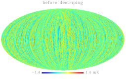
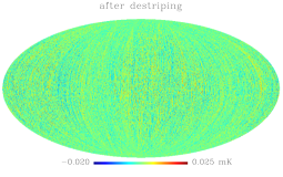
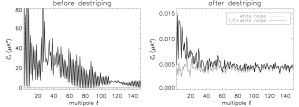
A destriping method can significantly reduce the $1/f$ noise. Anyway a residual contribution is still present after the correction. There are residual stripes in the map (Fig. 1), and in the angular power spectrum we can observe an excess of noise respect to the white noise level at low multipoles $\ell\lesssim 50$ (Fig. 2). Analytical studies have shown that the residual $1/f$ noise introduces a block-diagonal structure in the covariance matrix of the harmonic coefficients of the map. The off-diagonal terms have been found to be much smaller than the diagonal components, but not completely negligible in comparison to the tiny non-Gaussian signal we are looking for (Efstathiou, 2005). Therefore is important to investigate the impact of these correlations on the non-Gaussianity statistical tests.

Figure 1.— (top) Map of white and $1/f$ noise before destriping; (bottom) after destriping stripes are visible due to residual $1/f$ noise (the white noise contribution has been subtracted). We remark the different peak-to-peak values of the maps.

Figure 2.— The black line is the power spectrum of a map with white and $1/f$ noise before (right) and after (left) destriping (for $f_{k}=0.05$ Hz, $\alpha=1.7$). The gray line is the power spectrum of a map with only white noise. Note the different values range of the two plots.

2.3. The asymmetric beam

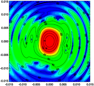
Actual CMB observation requires multi-frequency focal plane arrays to achieve proper angular resolution, sensitivity and spectral coverage. This is indeed the case of Planck, where we have the HFI focal plane, with $36$ horns, inserted into the ring formed by the $11$ LFI horns. As a consequence, some feed horn can not be located close to the focal plane center, so that the beam pattern is asymmetric rather than circular. Realistic Planck optical simulations of the feed horns coupled to the telescope (Sandri et al., 2004; Brossard et al., 2004) have shown that the main beam patterns are well fitted by an elliptical shape given by a bivariate Gaussian (Fig. 3). Moreover the finite response in time of the detectors leads to an elongation of the beam along the scan direction. The horns scan the sky mainly in the same direction, perpendicular to the ecliptic plane. Only the ecliptic poles are swept in several directions, which makes the effective beam more symmetric.

The convolution of the sky signal in a map $T(\hat{r})$ with the beam can be written in harmonic space as

$$T(\hat{r})=\sum_{\ell}\sum_{m=-\ell}^{m=\ell}B_{\ell m}a_{\ell m}Y_{\ell m}(\hat{r}),$$ (2)

where $Y_{\ell m}$ are the spherical harmonics and $B_{\ell m}$ and $a_{\ell m}$ are the harmonic expansions of the beam and the sky signal respectively. For a circular symmetric beam we have $B_{\ell m}=B_{\ell m^{\prime}}$, but if the beam is asymmetric $B_{lm}$ is no longer isotropic and it depends also on the azimuthal direction $m$ (Wu et al., 2001). The azimuthal dependence increases the deconvolution complexity and the computational cost, thus an exact deconvolution of an asymmetric beam is not straightforward. A beam not correctly measured and treated in the data analysis pipeline may artificially distort the underling structure of the CMB signal, introducing a spurious dependence on the azimuthal direction and messing up the isotropy of the field. We will investigate the impact of this effect in the non-Gaussianity searches (see Ashdown et al. (2009) for a study of the asymmetric beam impact on map-making).

Figure 3.— Main beam contour plot of one of the Planck-LFI 70 GHz feed horns (simulated assuming an ideal telescope). The dotted lines are the bivariate Gaussian fitting (color scale: -90$\div$0 dB).

3. Statistical tests of Non-Gaussianity

In this work we have made use of two qualitatively different statistical approaches to test non-Gaussianity. In the first approach no assumption is made about the non–Gaussian model, and the Gaussian hypothesis is tested. In the following we will refer to such tests as blind tests. In this work we have chosen to use the Spherical Mexican Hat Wavelet (SMHW) and the Minkowsky functionals (MF hereafter). This tests make use of Monte Carlo (MC) simulations to calibrate the Gaussian behavior. A departure from the MC calibration is interpreted as a non-Gaussian detection. The blind approach has the advantage to be model independent, but it has a weak statistical power, $i.e.$ it is difficult to interpret the meaning of an eventual detection of non-Gaussianity in the data. In order to put quantitative constraints on the non-Gaussianity level we have to adopt another approach. Testing specific non–Gaussianity arising from inflationary models we can put limits to the non-linearity parameter $f_{\rm NL}$. We have used a cubic statistic to estimate the $f_{\rm NL}$ parameter for both the local and the equilateral non-Gaussianity.

Given the difference in the two approaches, also the possible impacts of the systematic effects are different. For the blind tests the issue is in the MC calibration, since it is not computationally manageable to include the $1/f$ noise or the asymmetric beam in sets usually of thousands of simulations. Therefore the presence of the systematics in the data can in general cause departures from the MC calibration, that can lead to false non-Gaussian detections. Also in the non-blind cubic statistic it is often not feasible to take exactly into account the systematic effects, due to the complexity of the numerical or analytical treatment involved. A not accurate handling of the systematics can potentially introduce a bias in the estimated $f_{\rm NL}$. Even if on average the effect is zero, and there is no bias, the spurious correlations introduced by the systematics can increase the variance of the estimator. An example of this behavior is the effect of the anisotropic noise, which introduces correlations between small and large scales. If not corrected, these leads to a noticeable increase of the variance at high multipoles (Creminelli et al., 2006; Smith et al., 2009).

Before analysing the impact of the systematics effects, we will briefly describe the statistical methods applied in the study.

3.1. SMHW

The main idea of the wavelet technique is to decompose the temperature field into a set of coefficients, which contain information about the signal at a given position and scale. We can perform a continuous analysis, taking the scale and the position in a continuum of values. The wavelets are a convenient technique to study non–-Gaussianity, since the wavelet transform is linear. Thus the wavelet coefficients preserve the Gaussianity properties of the original field. Moreover they allow us to study the non-Gaussian features at different scales. In particular the SMHW enhances the non-Gaussian signatures with spherical symmetry. The SMHW is the extension to the sphere of the Euclidian Mexican Hat Wavelet (Cayón et al., 2000; Martínez-González et al., 2002). It is given by

$$\Psi(\theta;R) = \frac{1}{\sqrt{2\pi}R\,N}\left[1+\left(\frac{y}{2}\right)^{2}\right]^{2}\left[2-\left(\frac{y}{R}\right)^{2}\right]e^{-\frac{y^{2}}{2R^{2}}},$$ (3)

$$N(R) \equiv \left(1+\frac{R^{2}}{2}+\frac{R^{4}}{4}\right)^{1/2},$$

where $R$ is the scale, $(\theta,\phi)$ represent polar coordinates on the sphere, $(y\equiv 2\tan\frac{\theta}{2},\phi)$ are polar coordinates in the tangent plane to the North pole, and $N(R)$ is a normalisation constant. Given the temperature field on the sphere $T(\theta,\phi)$, the wavelet coefficients are defined as:

$$w(\theta,\phi;R)=\int d\theta^{\prime}\,d\phi^{\prime}\sin\theta^{\prime}\,\tilde{T}({\bf x}+{\bf\mu})\Psi(\theta^{\prime};R),\,$$ (4)

$${\bf x}=2\tan\frac{\theta}{2}(\cos\phi,\sin\phi),\,{\bf\mu}=2\tan\frac{\theta^{\prime}}{2}(\cos\phi^{\prime},\sin\phi^{\prime}).$$

Several statistics of the wavelet coefficients $w_{i}$ can be studied at a given scale $R$. In this work we have analyzed two simple non-Gaussian estimators: the skewness $S(R)$, $i.e.$ the degree of symmetry about the maximum, and the kurtosis $K(R)$, which indicates the degree to which a statistical frequency curve is peaked. Assuming zero mean at each scale we have:

$$S(R) = \frac{1}{N_{R}}\sum_{i=1}^{N_{R}}\left(\frac{w_{i}(R)}{\sigma(R)}\right)^{3}\,,$$ (5)

$$K(R) = \frac{1}{N_{R}}\sum_{i=1}^{N_{R}}\left(\frac{w_{i}(R)}{\sigma(R)}\right)^{4}-3,$$

where $\sigma^{2}(R)=\left(\sum_{i=1}^{N_{R}}w_{i}(R)^{2}\right)/N_{R}$ is the variance and $N_{R}$ is the number of coefficients (equal to the number of pixels $N_{pix}$ in our case).

3.2. Minkowski functionals

A general theorem of integral geometry states that the morphology of a convex body in $D$-dimensional space can be completely described by $D+1$ Minkowski functionals (Minkowski, 1903). In the case of the two-dimensional CMB field we consider the excursion sets $Q$, defined as the set consisting of the parts of the sky in which the temperature anisotropies amplitude $u$ is above a threshold $\nu$: $Q\equiv Q(\nu)=\{u|(u-\langle u\rangle)/\sigma_{0}>\nu\}$, where $\sigma_{0}^{2}=\langle u^{2}\rangle-\langle u\rangle^{2}$. Each of the functions has an explicit analytic expression for a Gaussian field (Tomita, 1986). Thus they provide an appropriate statistical test for Gaussianity. Different algorithms have been implemented to estimate the MF of a pixeled CMB sky map. In this work we have developed our algorithm following the approach of Eriksen et al. (2004), using the derivative computation of the HEALPix routines (Górski et al., 2005). The first functional, called the area functional, is defined as:

$$\mathcal{A}(\nu)=\frac{1}{A_{obs}}\int_{Q}dA\approx\frac{N_{pix}(u>\nu)}{N_{pix}^{\textrm{tot}}},$$ (6)

and is equal to the total area of $Q$. The second equality holds in the HEALPix pixelization, in which all pixels have exactly equal area. Then we define the length functional, $i.e.$ the total length of the boundary $\partial Q$ of the excursion set:

$$\mathcal{L}(\nu)=\int_{\partial Q}d\ell$$ (7)

where $\mathcal{L}$ is normalized to have a unit integral value: $\int\mathcal{L}(\nu)d\nu=1$. Finally the third functional is the genus, which measures the connectivity of $Q$, being equal to the number of isolated regions (hot spots) minus the numbers of holes (cold spots). It can be defined by:

$$\mathcal{G}(\nu)=\frac{N_{\rm{max}}(\nu)+N_{\rm{min}}(\nu)-N_{\rm{sad}}(\nu)}{N_{\rm{max}}(-\infty)+N_{\rm{min}}(-\infty)+N_{\rm{sad}}(-\infty)},$$ (8)

$i.e.$ as the number of maxima and minima minus the number of saddle points in the excursion set, divided by the sum of all stationary points in the whole un-thresholded field. In addition we use another morphological descriptor: the skeleton length, defined as the zero-contour line of the map $\mathcal{S}$:

$$\mathcal{S}=T_{;\phi}T_{;\theta}(T_{;\phi\phi}-T_{;\theta\theta})+T_{;\phi\theta}(T_{;\theta}^{2}-T_{;\phi}^{2}),$$ (9)

where semicolons denote the covariant derivatives. We compute the length of the skeleton of that part of the field that lies above some threshold $\nu$, normalized by the length of the skeleton of the whole un-thresholded field. The zero-contour lines of $\mathcal{S}$ can be interpreted as the set of lines that extend from extremum to extremum along lines of maximum or minimum gradient. For details of the MF algorithm see Eriksen et al. (2004).

3.3. $f_{\rm NL}$ estimator

The three-point correlation, or the bispectrum, function is the lowest-order statistic able to distinguish non-Gaussian from Gaussian perturbations. Indeed for Gaussian CMB the expectation value is exactly zero. Therefore we can look at the bispectrum as a natural observable to constrain the non–Gaussianity amplitude predicted by inflationary models, determined by the $f_{\rm NL}$ parameter. After measuring the bispectrum modes of a given map we can build a cubic estimator of $f_{\rm NL}$ in the following way:

$$\hat{f}_{\rm NL}=\frac{{\mathcal{S}}_{\rm prim}}{N}.$$ (10)

${\mathcal{S}}_{\rm prim}$ is a cubic statistic defined as

$${\mathcal{S}}_{\rm prim}=\sum_{\ell_{1}\leq\ell_{2}\leq\ell_{3}}\frac{\tilde{B}_{\ell_{1}\ell_{2}\ell_{3}}^{obs}\tilde{B}_{\ell_{1}\ell_{2}\ell_{3}}^{\rm prim}}{\tilde{C}_{\ell_{1}}\tilde{C}_{\ell_{2}}\tilde{C}_{\ell_{3}}},$$ (11)

where $\tilde{B}_{\ell_{1}\ell_{2}\ell_{3}}^{obs}$ is the bispectrum extracted from the observed map and $\tilde{B}_{\ell_{1}\ell_{2}\ell_{3}}^{\rm prim}$ is the ansatz for $f_{\rm NL}=1$ of the non-Gaussian model assumed, while $N$ is a normalisation factor defined as

$$N=\sum_{\ell_{1}\leq\ell_{2}\leq\ell_{3}}\frac{(\tilde{B}_{\ell_{1}\ell_{2}\ell_{3}}^{\rm prim})^{2}}{\tilde{C}_{\ell_{1}}\tilde{C}_{\ell_{2}}\tilde{C}_{\ell_{3}}},$$ (12)

where $\tilde{C}_{\ell}$ is the theoretical power spectrum of the model, after including the instrumental beam and noise.

We adopt the fast numerical implementation of the estimator in Eq. (10) found by Komatsu et al. (2005); Creminelli et al. (2006); Yadav et al. (2008); Smith & Zaldarriaga (2006). We consider two different primordial shapes of non–Gaussianity: local non–Gaussianity, in which we expect the major contributions to the bispectrum from squeezed configurations, where $\ell_{1}\ll\ell_{2},\ell_{3}$; and equilateral non–Gaussianity, which predict large bispectrum contributions for equilateral shapes, $i.e.$ for $\ell_{1}\sim\ell_{2}\sim\ell_{3}$. The corresponding $f_{\rm NL}$ estimators are described in the literature cited above. In the following subsections we recall the definitions of the main quantities involved.

3.3.1 local estimator

In the context of a local model of primordial non-Gaussianity it is useful to define the quantities

$$\alpha_{\ell}(r) \equiv \frac{2}{\pi}\int k^{2}dkg_{T\ell}(k)j_{\ell}(kr),$$ (13)

$$\beta_{\ell}(r) \equiv \frac{2}{\pi}\int k^{2}dkP(k)g_{T\ell}(k)j_{\ell}(kr),$$ (14)

where $g_{Tl}(r)$ is the radiation transfer function, $j_{l}(kr)$ is a Bessel function and $P(k)$ is the power–spectrum of the primordial perturbations. With these quantities we can obtain two filtered maps from the harmonic coefficients $a_{\ell m}$ of the observed CMB:

$$A(r,\hat{\mathbf{n}}) \equiv \sum_{\ell m}\frac{\alpha_{\ell}(r)W_{\ell}}{\tilde{C}_{\ell}}a_{\ell m}Y_{\ell m}(\hat{\mathbf{n}})\,,$$ (15)

$$B(r,\hat{\mathbf{n}}) \equiv \sum_{\ell m}\frac{\beta_{\ell}(r)W_{\ell}}{\tilde{C}_{\ell}}a_{\ell m}Y_{\ell m}(\hat{\mathbf{n}})\,,$$ (16)

where $W_{\ell}$ is the beam function of the instrument and $\tilde{C}_{\ell}$ is the theoretical power-spectrum $C_{\ell}$, after including effects of beam and noise as $\tilde{C}_{\ell}\equiv C_{\ell}W_{\ell}^{2}+\sigma_{0}^{2}$. Here we are approximating the noise as homogeneous $\left<n_{\ell m}n_{\ell^{\prime}m^{\prime}}^{*}\right>\simeq\sigma_{0}^{2}\delta_{\ell\ell^{\prime}}\delta_{mm^{\prime}}$. With these maps we can construct a cubic statistics (Komatsu et al., 2005)

$${\mathcal{S}}^{\rm local}_{\rm prim}\equiv 4\pi\int r^{2}dr\int\frac{d^{2}\hat{\mathbf{n}}}{4\pi}A(r,\hat{\mathbf{n}})B^{2}(r,\hat{\mathbf{n}}).$$ (17)

This expression reduces exactly to Eq. (11), so we can define the estimator of Eq. (10). In the case of full sky coverage and homogeneous noise, the estimator is fully optimal, $i.e.$ it saturates the Cramer-Rao bound, providing the minimum variance estimator. But it is not realistic to consider a full sky coverage. If $f_{sky}$ is the fraction of sky observed we multiply the normalisation $N$ of Eq. (12) by $f_{sky}N$ (Komatsu et al., 2005; Creminelli et al., 2006). Moreover in an experiment the noise results anisotropic, since different sky regions are observed for different amounts of time. Thus the noise covariance matrix $\left<n_{\ell m}n_{\ell^{\prime}m^{\prime}}^{*}\right>$ is no longer diagonal. The resulting correlation between small and large scales causes an increase of the variance of the estimator at high $\ell$’s. This can be corrected with a linear term defined by (Creminelli et al., 2006; Yadav et al., 2008)

$${\mathcal{S}}^{linear}_{\rm prim} =-\int r^{2}dr\int d^{2}\hat{\mathbf{n}}\Big{\{}2B(r,\hat{\mathbf{n}})\langle A_{sim}(r,\hat{\mathbf{n}})\cdot$$ (18)

$$B_{sim}(r,\hat{\mathbf{n}})\rangle_{MC}+\,A(r,\hat{\mathbf{n}})\langle B^{2}_{sim}(r,\hat{\mathbf{n}})\rangle_{MC}\Big{\}},$$

where $A_{sim}(r,\hat{\mathbf{n}})$ and $B_{sim}(r,\hat{\mathbf{n}})$ are the $A$ and $B$ maps generated from Monte Carlo simulations that contain signal and noise, and $\langle\dots\rangle$ denotes average over the simulations. The estimator is finally given by

$$\hat{f}^{\rm local}_{\rm NL}=\frac{{\mathcal{S}}^{\rm local}_{\rm prim}+{\mathcal{S}}^{linear}_{\rm prim}}{N},$$ (19)

This treatment greatly improves the final error bars of the estimator, but it does not yet provide fully optimality. This is achieved by Smith et al. (2009) through the implementation in Eq. (10) of the full covariance matrix.

3.3.2 equilateral estimator

In addition to $\alpha_{\ell}(r)$ and $\beta_{\ell}(r)$ (Eqs. (13,14)) we can define the functions

$$\gamma_{\ell}(r) \equiv \frac{2}{\pi}\int k^{2}dk{P(k)}^{1/3}g_{T\ell}(k)j_{\ell}(kr),$$ (20)

$$\delta_{\ell}(r) \equiv \frac{2}{\pi}\int k^{2}dk{P(k)}^{2/3}g_{T\ell}(k)j_{\ell}(kr)\;.$$ (21)

and obtain the filtered maps $C(r,\hat{\mathbf{n}})$ and $D(r,\hat{\mathbf{n}})$ in the same way of the maps $A(r,\hat{\mathbf{n}})$ and $B(r,\hat{\mathbf{n}})$ (Eqs. (15,16)). Now the statistics is given by (Creminelli et al., 2006)

$${\mathcal{S}}^{\rm equil}_{prim} = -18\int r^{2}dr\int d^{2}\hat{\mathbf{n}}\;\Big{[}A(r,\hat{\mathbf{n}})B^{2}(r,\hat{\mathbf{n}})$$ (22)

$$+ \frac{2}{3}D^{3}(r,\hat{\mathbf{n}})-2B(r,\hat{\mathbf{n}})C(r,\hat{\mathbf{n}})D(r,\hat{\mathbf{n}})\Big{]}$$

and the estimator results again $\hat{f}^{\rm equil}_{\rm NL}={\mathcal{S}}^{\rm equil}_{\rm prim}/N$, where $N$ is given by Eq. (12). In this case the anisotropic noise is not an issue, since the spurious effect is quite low for equilateral bispectrum configurations.

4. Analysis

In order to test the impact of the $1/f$ noise and the asymmetric beam we have analysed realistic Planck simulations of Gaussian CMB. The two systematic effects are studied separately, considering two different sets of Planck-like maps in which the $1/f$ noise or the asymmetric beam are simulated. For each systematic the test consists in a comparison of the results obtained on the realistic simulation set, with those obtained on another set of simulations hereafter dubbed “nominal”, in which the considered systematic is not present.

4.1. Simulation sets

Realistic Planck simulations can be obtained with the LevelS pipeline (Reinecke et al., 2006), an assembly of numerical tools specifically developed to model the output data of the Planck satellite. LevelS has been used to create simulations of the time-ordered-data (TOD) for the 12 radiometers of the LFI-70 GHz channel. The two systematic effects considered are expected to be stronger for the LFI channels. The choice in particular of the 70 GHz channel in our study let us work with the best sensitivity and angular resolution among the LFI channels. The TODs cover 1 year of mission. Every set of TODs has been then converted in a map, using the destriper map-making Springtide (Ashdown et al., 2007a), with $N_{side}=1024$ in the HEALPix pixelization scheme. For each systematic effect we have a set of 100 Planck-like maps. The size of the set is limited because of the large resources required by the TODs simulations and the subsequent map-making, both in terms of CPU computing time and disk space. We have to keep in mind this limited size when looking at the results. Nevertheless we have found that 100 maps are sufficient to obtain meaningful results. We describe now the characteristics specific of each set.

4.1.1 $1/f$ noise simulation set

For each radiometer the instrumental noise is simulated as a sum of white and $1/f$ noise, with PSD given by Eq. (1). The parameters adopted are reported in Table 1.

Table 1parameters adopted in the $1/f$ noise simulations

standard deviation	$\sigma=1787.6\,\mu$K
knee frequency	$f_{k}=50$ mHz
$1/f$ slope	$\alpha=1.7$
sampling frequency	$f_{s}=76.8$ Hz

Due to the Planck scanning strategy the noise is anisotropic. The white noise level chosen satisfies the goal sensitivity of the LFI-70 GHz channel (The Planck Collaboration, 2005). Subsequent tests on the 70 GHz radiometers have shown a lower knee frequency. Moreover comparative map-making methods studies have found that the residual noise is slightly higher for Springtide with respect to other destriping implementation (Ashdown et al., 2007a, b, 2009). Therefore these simulations are a conservative upper limit for the $1/f$ noise.

In addition to these 100 realistic noise maps, we have considered also a set of nominal simulations, $i.e.$ 100 white noise maps, in which the noise is a realization of anisotropic white noise with the same nominal standard deviation of the Planck simulations. To both noise map sets we have added 100 maps of Gaussian CMB sky. The CMB maps are random realizations of the $WMAP$-1 year best fit power spectrum, convolved with the angular resolution of the LFI-70 GHz channel with a circular Gaussian beam of $14^{\prime}$. Finally, for the SMHW and the MF analyses we need Monte Carlo (MC) simulations for calibration. Thus we have created 5000 MC maps of anisotropic white noise and Gaussian CMB. We remark that the MC calibration does not contain the $1/f$ noise.

4.1.2 asymmetric beam simulation set

The LevelS pipeline has been used to simulate a Planck-like observation of 100 Gaussian CMB skies, created as random realizations of the $WMAP$-1 year best fit power spectrum. The sky observation is simulated considering the best-fit elliptical beams of the LFI-70 GHz, obtained in realistic main beam simulations (Sandri et al., 2004). The parameters of the bivariate Gaussian fitting for each radiometer are reported in Table 2. The twelve radiometers form symmetric couples due to the symmetry of the LFI focal plane.

Table 2parameters adopted in the asymmetric beam simulations

id	FWHM	ellipticity
18a, 23a	13.0328	1.2601
18b, 23b	12.9916	1.2184
19a, 22a	12.7053	1.2509
19b, 22b	12.6494	1.2162
20a, 21a	12.4795	1.2460
20b, 21b	12.4273	1.2224

The sampling in time has been also simulated. Since the effect is a widening of the beam in the scan direction, it has been reproduced using a beam smeared in the rotation direction, perpendicular to the ecliptic plane.

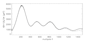
Furthermore we have created a set of 100 nominal simulations of Gaussian CMB, made again as random realizations of the $WMAP$-1 year best fit power spectrum, but in this case convolved with a circular Gaussian beam of $13^{\prime}$. This is the resolution of the symmetric beam which best approximates the asymmetric one (Fig. 4).

Figure 4.— Average power spectrum of 100 realistic simulations with asymmetric beam deconvolved with a circular Gaussian beam of $13^{\prime}$ (black line). The theoretical CMB spectrum is shown with a dashed line.

For some analysis we have also added a random realization of anisotropic white noise to each CMB map of both sets. The nominal standard deviation per sample is $\sigma=1787.6\,\mu$K (as in Table 1). We have finally created 5000 MC simulations to calibrate the SMHW and the MF analyses, following the same recipe of the nominal simulations.

4.2. SMHW analysis

We have calculated the wavelets coefficients $w_{i}$ at 18 different scales $R$, starting from the pixel size: $R=$ $3.4$, $6.9$, $10$, $13.7$, $25$, $50$, $75$, $100$, $150$, $200$, $250$, $300$, $400$, $500$, $600$, $750$, $900$, and $1050$ arcm. For each scale we have computed standard deviation $\sigma(R)$, skewness $S(R)$ and kurtosis $K(R)$ of the distribution of the coefficients (Eqs. (5)). For both the $1/f$ noise and the asymmetric beam analysis, the statistics are calculated on the 100 realistic simulations containing the systematic effect and on the 100 nominal simulations without it. For calibration we have also calculated $\sigma(R)$, $S(R)$ and $K(R)$ over 5000 MC simulations.

Since the distribution of the MC values is close to Gaussian, for every statistic and map we can construct a $\chi^{2}$ test in this form:

$$\chi^{2}(n)=\left({\bf x}(n)-\langle{\bf x}_{\rm MC}\rangle\right)^{T}{\bf C}^{-1}_{\rm MC}\left({\bf x}(n)-\langle{\bf x}_{\rm MC}\rangle\right),$$ (23)

where the vector ${\bf x}$ has elements $x_{i}=\sigma(R_{i})$, $S(R_{i})$ or $K(R_{i})$ and ${\bf C}^{-1}_{\rm MC}$ is the MC covariance matrix $C_{ij}=\langle\left(x_{i}-\langle x_{i}\rangle\right)\left(x_{j}-\langle x_{j}\rangle\right)\rangle$. The $\chi^{2}$ test is performed on each map of the realistic and of the nominal simulation sets, with $n=1-100$, and on each MC map, with $n=1-5000$. Moreover we have established the acceptance intervals at different significance levels $\alpha$ for each statistic $\sigma(R)$, $S(R)$ or $K(R)$ and scale. Fixing $R$, we look at the distribution of the values over the 5000 MC maps: an acceptance interval is defined as the one containing a percentage $1-\alpha$ of values, where the remaining percentage is the same above and below the interval, $i.e.$ $\alpha/2$ at each side. We have chosen three significance levels: $68$% ($1\sigma$), $5$% ($2\sigma$) and $1$%. When a value falls out of an interval, the significance of the non-Gaussianity indication is given by $\alpha$: lower is the significance level $\alpha$, stronger is the indication.

With these quantities we have constructed three figures of merit. Each figure is evaluated for standard deviation $\sigma(R)$, skewness $S(R)$ and kurtosis $K(R)$ on both the realistic and the nominal simulation sets. We have looked at all the three statistics, but remembering that only skewness and kurtosis are Gaussian estimators. We have also studied the standard deviation for a better characterisation of the systematic effect.

1. $\chi^{2}$ distributions comparison:
   We have tested if the 100 $\chi^{2}$ values of the simulation set belong to the same distribution of 5000 $\chi^{2}_{\rm MC}$ values of the MC simulations. The degree of agreement is quantified as the percentage of $\chi^{2}_{\rm MC}$ greater than the mean of the $\chi^{2}$ of the 100 simulations;

2. number of $\chi^{2}$ out of $2\sigma$:
   For each $\chi^{2}$ value of the simulation set we have looked at the percentage of MC simulations with a lower $\chi^{2}_{\rm MC}$. If this percentage is less than $2.5$% or more than $97.5$%, then the $\chi^{2}$ value lies outside $2\sigma$ of the $\chi^{2}_{\rm MC}$ distribution;

3. number of outliers:
   For each scale we have counted the number of maps with statistic of the wavelet coefficients out of the acceptance intervals at $5$% and $1$%.

The impact of the $1/f$ noise or the asymmetric beam has been tested comparing the figures of merit of the realistic simulation set against the figures of the nominal one.

4.2.1 SMHW: $1/f$ noise results

The first figure of merit for the $1/f$ noise is showed in Fig. 5.

Figure 5.— SMHW - $1/f$ noise results: $\chi^{2}$ distributions comparison for realistic (top line) and nominal (bottom line) simulations. The dot-dashed line shows the $\langle\chi^{2}\rangle$ of the simulation set. We indicate the percentage of $\chi^{2}_{\rm MC}$ greater than this mean.

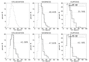
The impact of the $1/f$ is noticeable only in the standard deviation: the $\chi^{2}$ distribution of the realistic set is not displayed in the plot because the values are out of range respect to the MC set (upper-left plot in Fig. 5). This is indeed expected, because of the increase of the noise variance with respect to the white noise level of the MC calibration due to the $1/f$ noise contribution. All the other plots show an agreement between the set of maps and the MC calibration, indicated also by the percentage of $\chi^{2}_{\rm MC}$ greater than the $\chi^{2}$ mean. Table 3 reports the second figure of merit. Apart again from the standard deviation, the $1/f$ noise does not increase the occurrence of skewness or kurtosis out of $2\sigma$ from the Gaussian behavior as calibrated with MC simulations.

Table 3SMHW - $1/f$ noise results: number of $\chi^{2}$ out of $2\sigma$

# of $\chi^{2}$	std.deviation	skewness	kurtosis
realistic	100	3	3
nominal	1	5	7

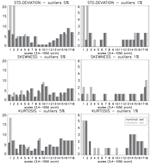
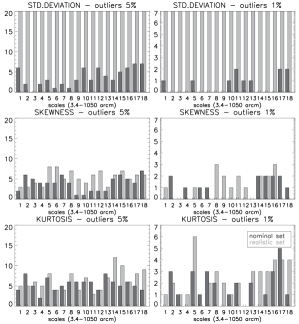
The third figure of merit (Fig. 6) shows the impact of the $1/f$ noise on the different scales. We can observe that at scales $R\sim$ pixel scale the presence of $1/f$ noise increase the probability for a map to have the standard deviation of wavelet coefficients out of $1$% or $5$%. Actually this scale is noise dominated and usually it is not considered in Gaussianity analysis.

Before moving on in the analysis, a general comment on the third figure of merit is mandatory. We can sometime observe a number of outliers greater than what expected in particular for the nominal set, since these maps are obtained with the same pipeline of the MC simulations. This is only due to the limited size of the simulation sets, which increases the number of values in the distribution tails.

Figure 6.— SMHW - $1/f$ noise results: number of outliers of the $5$% and $1$% acceptance intervals.

We have repeated the analysis also with an amplified noise contribution: in both the realistic and the nominal simulation sets the noise maps have been multiplied by a factor equal to $2.5$. The results found are qualitatively unchanged, thus we do not show them here.

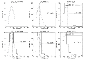
For a better understanding of the noise properties we finally have analysed only noise simulation, in which no CMB signal is added. We can look at the $\chi^{2}$ test of the realistic simulations in Fig. 7. Apart from the standard deviation, where again we have obtained values out of MC set range, only the kurtosis shows a somewhat lower percentage for the realistic set respect to the nominal one. Anyway the value still indicates a good agreement with the MC distribution. Also the number of $\chi^{2}$ out of $2\sigma$ reported in Table 4 is not affected by the $1/f$ noise contribution.

Figure 7.— SMHW - $1/f$ noise results: $\chi^{2}$ distributions comparison [only noise simulations] for realistic (top line) and nominal (bottom line) simulations. The dot-dashed line shows the $\langle\chi^{2}\rangle$ of the simulation set. We indicate the percentage of $\chi^{2}_{\rm MC}$ greater than this mean.

But when we look at the third figure of merit in Fig. 8, we can see that the $1/f$ noise increases the number of outliers. The standard deviation is affected at all the scales, since here the increase of noise variance is no more hidden by any CMB signal. Also skewness and kurtosis are affected at some scales, but we observe that the number of outliers remains within statistically reasonable limits.

Table 4SMHW - $1/f$ noise results: number of $\chi^{2}$ out of $2\sigma$ [only noise simulations]

# of $\chi^{2}$	std.deviation	skewness	kurtosis
realistic	100	3	4
nominal	4	4	7

Figure 8.— SMHW - $1/f$ noise results: number of outliers [only noise simulations]

4.2.2 SMHW: asymmetric beam results

Figure 9.— SMHW - asymmetric beam results: $\chi^{2}$ distributions comparison for realistic (top line) and nominal (bottom line) simulations. The dot-dashed line shows the $\langle\chi^{2}\rangle$ of the simulation set. We indicate the percentage of $\chi^{2}_{\rm MC}$ greater than this mean.

The first figure of merit in Fig. 9 shows that the asymmetric beam has an impact on the standard deviation: the $\chi^{2}$ values of the realistic set are out of range with respect to the MC set values. We can see in Fig. 4 that indeed the elliptical beam used in the realistic simulation produces a different smoothing with respect to the circular beam, used in the nominal and in the MC simulations. Instead skewness and kurtosis percentages indicate a still good agreement with the MC calibration, even if lower with respect to the symmetric beam maps. The number of $\chi^{2}$ out of $2\sigma$ in Table 5 confirms that the asymmetric beam has a significant impact on the $\chi^{2}$ distribution of the standard deviation statistic only.

Table 5SMHW - asymmetric beam results: number of $\chi^{2}$ out of $2\sigma$

# of $\chi^{2}$	std.deviation	skewness	kurtosis
realistic	100	3	6
nominal	8	4	4

Figure 10.— SMHW - asymmetric beam results: number of outliers

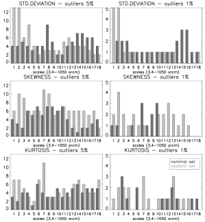
Looking at the number of outliers in Fig. 10 we observe that the asymmetric beam increases the occurrence of wavelet coefficients statistics out of the acceptance intervals. This happens only at small scales for the standard deviation, while we have a general slight increase for kurtosis and skewness. Anyway for these two statistics the numbers of outliers are still admissible and the departure from the MC Gaussian calibration is not significant. We have repeated the analysis adding an anisotropic white noise to the CMB maps, both in the realistic and in the nominal simulation sets. We have found that the noise does not modify the impact of the asymmetric beam and the results do not change.

4.3. MF analysis

In order to investigate different angular scales, for both the $1/f$ noise and the asymmetric beam study we have smoothed the sets of 100 simulations, realistic and nominal, with Gaussian beams at $0$ ($i.e.$ no smoothing), $10$, $30$, $60$, $120$, $180$ and $240$ arcm. For every map and smoothing scale we then have estimated the MF, $i.e.$ area, length, genus and skeleton length. The derivative computation is performed up to an appropriate multipole $\ell_{max}$ for each scale: from $850$ to $60$ for the larger beam. The MF are estimated for $200$ threshold values $\nu=-4\sigma\div 4\sigma$, but in the subsequent analysis we consider only thresholds $-3\sigma<\nu<3\sigma$ ($-2.5\sigma<\nu<2.5\sigma$ for the two larger scales). We have applied the same procedure to the 5000 MC maps for calibration. Having verified the Gaussianity of the values distribution over the MC, we have constructed a $\chi^{2}$ test. We have performed a diagonal $\chi^{2}$ test, due to the narrow step-size used in the thresholds range, defining

$$\chi^{2}(n)=\sum_{\nu}\left[\frac{f(\nu,n)-\langle f_{\rm MC}(\nu)\rangle}{\sigma_{\rm MC}(\nu)}\right]^{2},$$ (24)

where $f$ is one of the MF, $\langle f_{\rm MC}(\nu)\rangle$ and $\sigma_{\rm MC}(\nu)$ are the mean and the standard deviation over the MC simulations. The $\chi^{2}$ test has been performed on the realistic and the nominal simulation sets and on the MC calibration maps.

The evaluation of the results is achieved analysing two figures of merit, identical to the first two figures considered in the SMHW analysis in §4.2, $i.e.$:

1. $\chi^{2}$ distributions comparison;

2. number of $\chi^{2}$ out of $2\sigma$.

The figures of merit are evaluated for each smoothing scale and functional. For both the $1/f$ noise and the asymmetric beam study, we are going to compare the results of the figures obtained on the realistic and on the nominal simulation set, $i.e.$ respectively with or without the systematic considered.

4.3.1 MF: $1/f$ noise results

Figure 11.— MF - $1/f$ noise results: $\chi^{2}$ distributions comparison

Figure 12.— MF - $1/f$ noise results: number of $\chi^{2}$ out of $2\sigma$.

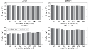
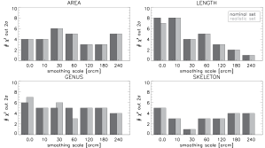
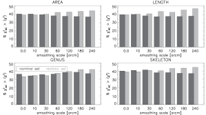
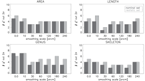
In the first figure of merit (Fig. 11) it is straightforward to see that there is not any noticeable difference between the results obtained with the $1/f$ noise included and the results from the nominal simulations, in none of the smoothing scales applied to the maps. Also looking at the number of $\chi^{2}$ out of $2\sigma$ in Fig. 12, we can say that the agreement of the simulation set with the MC calibration is not affected by the $1/f$ noise. We have checked the robustness of the results repeating the analysis on simulations with an higher noise level. The noise maps, both in the nominal and in the realistic simulation set, have been multiplied by a factor of $2.5$. The results found are almost identical to that showed.

4.3.2 MF: asymmetric beam results

Comparing the distribution of $\chi^{2}$ values of the simulation sets with the MC calibrations (Fig. 13), we observe that the asymmetric beam of the realistic simulations does not cause a lower agreement with respect to the nominal simulations. In Fig. 14 we can see that for the asymmetric beam maps in many cases we have found more $\chi^{2}$ values out of $2\sigma$ respect to the symmetric beam maps, but the increase is not remarkable. We have also analysed the same CMB simulations after adding anisotropic white noise, but the results do not change significantly.

Figure 13.— MF - asymmetric beam results: $\chi^{2}$ distributions comparison

Figure 14.— MF - asymmetric beam results: number of $\chi^{2}$ out of $2\sigma$

4.4. $f_{\rm NL}$ estimator analysis

Figure 15.— $f_{\rm NL}^{\rm local}$ - $1/f$ noise results. Error bars and standard deviations are $1\sigma$.

Figure 16.— $f_{\rm NL}^{\rm equil}$ - $1/f$ noise results

Figure 17.— $f_{\rm NL}^{\rm local}$ - asymmetric beam results

Figure 18.— $f_{\rm NL}^{\rm equil}$ - asymmetric beam results

Figure 19.— $f_{\rm NL}^{\rm local}$ - asymmetric beam results [with anisotropic noise]

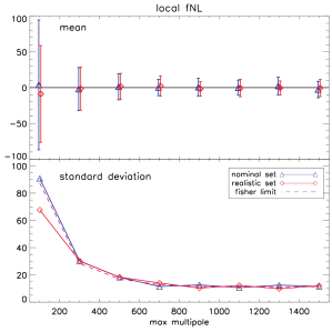
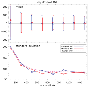
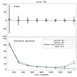
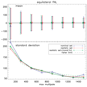
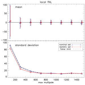
In order to test the impact of the $1/f$ noise and the asymmetric beam on the $f_{\rm NL}$ parameter, we have performed the estimation with the cubic statistic described in §3.3 on the realistic and the nominal simulation sets, in both the local and the equilateral configuration. In the local configuration, when the noise is added, we have also corrected for correlations introduced by the anisotropic noise, computing the linear term of Eq. (18). The bispectrum is calculated up to different maximum values of multipole $\ell_{max}$. We have proceeded looking at the mean of the $f_{\rm NL}$ values obtained, to check against biases with respect to the expected null value. Then we have investigated the impact of the systematic effects on the variance of the estimator, comparing the standard deviations of the two sets of 100 $f_{\rm NL}$ values obtained from the realistic and the nominal simulations.

4.4.1 $f_{\rm NL}$: $1/f$ noise results

As explained in §3.3, correlation properties of the noise random field have to be properly accounted for, introducing correction terms, like the linear term of Eq. (18); or computing the full noise covariance matrix and performing an inverse covariance matrix weighting of the data (Smith et al., 2009). But in the case of the $1/f$ noise the estimation of the noise covariance matrix is numerically challenging, in particular at the high resolution reached with Planck (see Keskitalo et al. (2009) for the study of the noise covariance matrix for Planck low-resolution data analysis). Before making any attempt in this direction, it is therefore useful to evaluate the effective impact of the $1/f$ noise without accounting for it in the $f_{\rm NL}$ estimation. Actually the noise is considered in the computation of the Fisher matrix $N$ (Eq. 12) and of the maps $A(r,\hat{\mathbf{n}})$, $B(r,\hat{\mathbf{n}})$, $C(r,\hat{\mathbf{n}})$ and $D(r,\hat{\mathbf{n}})$ (Eqs. (15, 16)), but it is accounted by means of its power spectrum, therefore without considering the correlations introduced by the $1/f$ noise in the realistic simulations.

In Fig. 15 we show the results for the local configuration, while in Fig. 16 there are the equilateral configuration results. In both the cases we can not observe any bias in the mean of $f_{\rm NL}$. This is indeed expected, since the $1/f$ noise is correlated but still Gaussian. But it is important to check against possible biases introduced by the not proper noise treatment itself. Moreover the $1/f$ noise does not increase the $f_{\rm NL}$ standard deviation, and the error bars have the same amplitude obtained from the nominal simulations. The small deviations between the obtained values and the limit given by the Fisher matrix are compatible due to the limited size of the simulation sets.

4.4.2 $f_{\rm NL}$: asymmetric beam results

We can repeat here the same considerations made for the $1/f$ noise. The asymmetric beam can introduce correlations in the data, but the numerical description of this effect is demanding. Therefore we want to evaluate the effective impact of this systematic when it is not properly accounted for. In the estimation of $f_{\rm NL}$ the beam considered in the computation is circular. In particular we have considered a circular Gaussian beam of $13^{\prime}$, the same used in the nominal simulation.

The results obtained for the local and the equilateral $f_{\rm NL}$ are shown in Fig. 17 and Fig. 18 respectively. Looking at the mean of the $f_{\rm NL}$ values, not any bias is observable with respect to the null value in both the configurations. For the equilateral case, the standard deviation is also not affected by the asymmetric beam. In contrast in the local configuration we can observe an increase of the standard deviation at high multipoles.

In order to understand if this increase is due only to the different smoothing of the elliptical beam with respect to the circular one, we have applied a transfer function in the $f_{\rm NL}$ estimation. This function is calculated as the mean of the spectra of the realistic simulation set, divided by the theoretical spectrum convolved with the circular $13^{\prime}$ beam. Therefore the “effective” beam, obtained as the circular beam multiplied for this transfer function, has the same amplitude of the elliptical beam. We have used this “effective” beam in the $f_{\rm NL}$ estimation of the asymmetric beam maps. The results obtained using the transfer function are shown in green color in the same Figs. 17 and 18. We can observe that, even if lower, the increase in the standard deviation of the local configuration is still present.

Then we have analyzed the same simulations after adding an anisotropic white noise contribution to the CMB maps. This is indeed a more realistic situation. The noise does not change the results for the equilateral configuration. On the other hand the standard deviations of the local $f_{\rm NL}$ are significantly improved with respect to the situation without noise. We show that the local configuration results in Fig. 19: the increase of the error bars at high multipoles is no longer observable.

5. Conclusions

We have studied the impact of the $1/f$ noise and the asymmetric beam on searches for non-Gaussian primordial signals. These two systematics effects are indeed expected to be present in the forthcoming Planck CMB data. With realistic Planck-like simulations we have evaluated if they can affect the non-Gaussianity analysis carried out with different statistical approach: blind tests, as the SMHW and the Minkowski functionals, and an $f_{\rm NL}$ estimator for both local and equilateral configurations, known as the “KSW” estimator. The two systematics have been studied separately. In the case of the blind tests we have looked at different figures of merit, checking for false non-Gaussian detections, while for the $f_{\rm NL}$ estimator we have checked for the bias in the estimated value and for the increase in the variance. In each case the results on realistic simulations have been compared with the results on simulations without the systematic effect examined.

For both the $1/f$ noise and the asymmetric beam analysis, no tests conducted shows a significant impact on the final results. The $1/f$ noise can slightly affect only the SMHW analysis, and only when the noise dominates over the CMB signal, $e.g.$ at pixel scale. The blind tests are not significantly affected by the non circular beam, but in the case of the $f_{\rm NL}$ estimator we can observe an increase of the variance of the local $f_{\rm NL}$ at high multipoles, when we consider simulations without noise. Anyway this effect is canceled once we consider more realistic noisy simulations.

In conclusion, assuming that the simulations analysed well reproduce the actual Planck observations, if any non–Gaussian signal will be detected in the forthcoming Planck CMB data with these statistical tests, it will not be due to the 1/f noise or the asymmetry of the beam.

References

- Acquaviva et al. (2003) Acquaviva V., Bartolo N., Matarrese S., and Riotto A., Nucl. Phys. B 667 (2003) 119.
- Ashdown et al. (2007a) Ashdown M.A.J. et al., A&A 467 (2007) 761.
- Ashdown et al. (2007b) Ashdown M.A.J. et al., A&A 471 (2007) 361.
- Ashdown et al. (2009) Ashdown M.A.J. et al., A&A 493 (2009) 753.
- Babich et al. (2004) Babich D., Creminelli P. and Zaldarriaga M., JCAP 8 (2004) 9.
- Bartolo et al. (2001) Bartolo N., Komatsu E., Matarrese S., and Riotto A., Phys. Rep. 402 (2004) 103.
- Brossard et al. (2004) Brossard J. et al., Proc. of the 5th International Conference on Space Optics (ICSO 2004), ESA SP-554 (2004) 333.
- Cayón et al. (2000) Cayón et al., MNRAS 315 (2000) 757.
- Chen et al. (2007a) Chen X., Huang M.-X., Kachru S., and Shiu G., JCAP 0701 (2007) 002.
- Chen et al. (2007b) Chen X., Easther R., and Lim E.A., JCAP 0706 (2007) 023.
- Creminelli et al. (2006) Creminelli P., Nicolis A., Senatore L., Tegmark M., and Zaldarriaga M., JCAP 0605 (2006) 4.
- Curto et al. (2009) Curto, A., Martínez-González E., Mukherjee P., Barreiro R.B., Hansen F.K., Liguori M., and Matarrese S., MNRAS 393 (2009) 615.
- Efstathiou (2005) Efstathiou G., MNRAS 356 (2005) 1549.
- Eriksen et al. (2004) Eriksen H.K., Novikov D.I., Lilje P.B., Banday A.J., and Górski K.M., MNRAS 612 (2004) 64.
- Górski et al. (2005) Górski K.M., Hivon E., Banday A.J., Wandelt B.D., Hansen F.K., Reinecke M., and Bartelmann M., ApJ 622 (2005) 759.
- Hansen et al. (2009) Hansen F.K., Banday A.J., Górski K.M., Eriksen H.K., and Lilje P.B., ApJ 704 (2009) 1448 (arXiv:0812.3795).
- Holman & Tolley (2008) Holman R. and Tolley A.j., JCAP 0805 (2008) 001.
- Janssen et al. (1996) Janssen M. et al., Report PSI-96-01, FIRE-96-01 (1996) (arXiv:astro-ph/9602009).
- Keihänen et al. (2004) Keihänen E., Kurki-Suonio H., Poutanen T., Maino D., and Burigana C., A&A 428 (2004) 287.
- Keskitalo et al. (2009) Keskitalo R. at al., (2009), arXiv:0906.0175.
- Komatsu & Spergel (2001) Komatsu E. and Spergel D.N., Phys. Rev. D 63 (2001) 063002.
- Komatsu et al. (2005) Komatsu E., Spergel and Wandelt B.D., ApJ 634 (2005) 14.
- Komatsu et al. (2009) Komatsu E. et al., ApJS 180 (2009) 330.
- Langlois et al. (2008) Langlois D., Renaux-Petel S., Steer D.A., and Tanaka T., Phys. Rev. D 78 (2008) 063523.
- Linde & Mukhanov (1997) Linde A. and Mukhanov V., Phys. Rev. D 56 (1997) 535.
- Lyth et al. (2003) Lyth D.H., Ungarelli C, and Wands D., Phys. Rev. D 67 (2003) 023503.
- Maino et al. (2002) Maino D., Burigana C., Górski K. M., Mandolesi N., and Bersanelli M., A&A 387 (2002) 356.
- Maldacena (2003) Maldacena J., JHEP 0305 (2003) 013.
- Martínez-González et al. (2002) Martínez-González E., Gallegos J.E., Argüeso F., Cayón L., and Sanz J.L, MNRAS 336 (2002) 22.
- McEwen et al. (2008) McEwen J.D., Hobson M.P., Lasenby A.N., and Mortlock D.J., MNRAS 388 (2008) 659.
- Minkowski (1903) Minkowski H., Mathematische Annalen 57 (1903) 447.
- Pietrobon et al. (2009) Pietrobon D., Cabella P., Balbi A., de Gasperis G., and Vittorio N., MNRAS 396 (2009) 1682.
- Reinecke et al. (2006) Reinecke M., Dolag K., Hell R., Bartelmann M., and Enßlin T.A., A&A 445 (2006) 373.
- Rudjord et al. (2009) Rudjord Ø, Hansen F.K., Lan X., Liguori, M., Marinucci D., and Matarrese S., ApJ 701 (2009) 369 (arXiv:0901.3154).
- Sandri et al. (2004) Sandri M., Villa F., Mandolesi N., Bersanelli M., and Nesti R., Optical, Infrared, and Millimeter Space Telescopes., Proc. SPIE 5487 (2004) 532.
- Senatore et al. (2009) Senatore L., Smith K.M., and Zaldarriaga M., (2009), arXiv:0905.3746.
- Smith & Zaldarriaga (2006) Smith K.M. and Zaldarriaga M., arXiv:astro-ph/0612571.
- Smith et al. (2009) Smith K.M., Senatore L., and Zaldarriaga M., JCAP 0909 (2009) 006 (arXiv:0901.2572).
- The Planck Collaboration (2005) The Planck Collaboration, ESA-SCI(2005) [arXiv: astro-ph/0604069]
- Tomita (1986) Tomita H., Progr. Theor. Phys. 76 (1986) 952.
- Vielva et al. (2004) Vielva P. Martínez-González E., Barreiro R.B., Sanz J.L., and Cayón L., ApJ 609 (2004) 22.
- Yadav et al. (2008) Yadav A.P.S., Komatsu E., Wandelt B.D., Liguori M., Hansen F.K., and Matarrese S., ApJ 678 (2008) 578. 1
- Yadav & Wandelt (2008) Yadav A.P.S. and Wandelt B.D., Phys. Rev. Lett. 100 (2008) 181301.
- Wu et al. (2001) Wu J.H.P. et al., ApJS 132 (2001) 1.