Yangian symmetry in molecule {V6} and four-spin Heisenberg model

Abstract

The symmetry operator $Q=Y^{2}$ is introduced to re-describe the Heisenberg spin triangles in the {V6} molecule, where $\mathbf{Y}$ stands for the Yangian operator which can be viewed as special form of Dzyaloshiky-Moriya (DM) interaction for spin 1/2 systems. Suppose a parallelogram Heisenberg model that is comprised of four $\frac{1}{2}$-spins commutes with $Q$, which means that it possesses Yangian symmetry, we show that the ground state of the Hamiltonian $H_{4}$ for the model allows to take the total spin $S=1$ by choosing some suitable exchange constants in $H_{4}$. In analogy to the molecular {V6} where the two triangles interact through Yangian operator we then give the magnetization for the theoretical molecule “{V8}” model which is comprised of two parallelograms. Following the example of molecule {V15}, we give another theoretical molecule model regarding the four $\frac{1}{2}$-spins system with total spin $S=1$ and predict the local moments to be $\frac{9}{10}\mu_{B}$, $\frac{1}{10}\mu_{B}$, $\frac{1}{10}\mu_{B}$, $\frac{9}{10}\mu_{B}$ respectively.

1 Introduction

The single molecular magnets(SMMs)have attracted much attention both for its scientific importance of studying fundamental issues and for its potential applications. The magnetic molecules {V6} and {V15} provide us a good platform for exploring these issues for the models whose total spins are not large. There have been beautiful investigations on these respects.[1, 2, 3, 4]

For latter use, let us briefly introduce the structures of the molecule {V6} first. As was mentioned in the Ref.[2], the molecular {V6} is the abbreviation of the molecule (CN₃H₆)₄Na₂[H₄V₆O₈(PO₄)₄{(OCH₂)₃CCH₂OH}₂]$\cdot$ 14H₂O whose structure is shown in Fig.1. We see that the molecule consists of two pieces, each of which is an isosceles triangle. In each triangle, two of the spin exchange constants are equal(shown in blue $J_{a}\sim 65K$) and the third one is smaller(shown in red $J_{c}\sim 7K$).[3] The experiment has shown that there is a kind of special interaction called Dzyaloshiky-Moriya (DM) interaction[5] between the two triangles, whose Hamiltonian can be written as $H_{inter}=\Delta(\mathbf{S}_{A}\times\mathbf{S}_{A^{\prime}})_{y}$.[2] The operators $\mathbf{S}_{A}$ and $\mathbf{S}_{A^{\prime}}$ are the total spin operators of two triangles, respectively, and the energy gap $\Delta$ is tiny. However, such an interaction can make contributions to the Landau-Zener-Stückelberg (LZS) transition[6] when the magnetic field is absent. The LZS effect can be detected by measuring the magnetization of the molecule {V6}.[2]

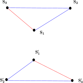
Figure 1: (color online)The structure model of {V6} molecule. The blue lines represent the two equal exchange interaction constants called $J_{a}$, and the red line is the third exchange interaction constant $J_{c}$. There is DM interaction $H_{inter}=\Delta(\mathbf{S}_{A}\times\mathbf{S}_{A^{\prime}})_{y}$ between the two triangles.

In Ref.[1, 2, 3, 4], the wave functions of molecule {V6} and the experimental measurements of the system have been shown clearly. However, from the theoretical point of view, each triangle of the molecule {V6} is formed by three spins, and the symmetry properties of the triangle desire to be investigated. In this article, we first focus on triangle of a molecule {V6}, and introduce a new symmetry operator $Q$ to re-describe the triangular piece. We can see that the commutativity between such a new symmetry operator $Q$ and the Hamiltonian of the triangle $H_{3}$ will constrain the parameters in $H_{3}$ leading to $J_{12}=J_{23}$(see Eq.(3)). The symmetry operator $Q$ looks a natural description for the triangle model in the molecular {V6}. Further we shall extend such a new symmetry to a four-spin Heisenberg model. Using the extended symmetry operator $Q$ in the four-spin system, the Hamiltonian $H_{4}$ for a parallelogram will be restricted. By analyzing the Hamiltonian $H_{4}$, we find that the ground state can be with total spin $S=1$ in some special cases, which has not been considered before. Based on this assumption, we make a prediction on the magnetization of a theoretical molecule “{V8}” which is comprised of two parallelograms with the DM interaction between them in analogy to the molecule {V6}.[2] To test the parallelogram model itself, we propose another molecular model in analogy to {V15} and give the prediction of its local spin moments configuration.

This article is organized as follows: In Sec.2,we shall investigate the single Heisenberg spin triangle model in {V6} and introduce the new quantum number operator $Q$ to re-describe the model. We shall show that the operator $Q$ represents a new symmetry in the three-spin system. In Sec.3, we shall extend the symmetry to a system comprised of four $\frac{1}{2}$-spins and establish its Hamiltonian $H_{4}$. We demonstrate that the ground state of $H_{4}$ allows to be with total spin $S=1$ in some special cases. Besides, we make up a theoretical molecular model called “{V8}” in which the Yangian interaction between the two parallelograms is introduced and the prediction of its magnetization is made. In Sec.4, we discuss another molecular model which contains only one parallelogram and give the prediction about its local spin moments configuration. In the Appendix, we shall show details about how the symmetry operator determines the Hamiltonian.

2 The new symmetry in {V6}

As was mentioned in the Sec.1, a molecule {V6} is comprised of two triangles with a tiny DM interaction between them. In this section, we shall concentrate on only one triangular piece in a molecule {V6}. It has been verified that the triangle model is actually isosceles by the experiment.[3] Hence the {V6} problem has been well-established both theoretically and experimentally. However, in this section we would like to introduce a new symmetry operator $Q$ to re-describe the triangle system that can be extended to more $\frac{1}{2}$-spins system.

The model of the Heisenberg spin triangle is comprised of there spin-$\frac{1}{2}$ particles, whose Hamiltonian is written as:

$$H_{0}=J_{12}\mathbf{S}_{1}\cdot\mathbf{S}_{2}+J_{23}\mathbf{S}_{2}\cdot\mathbf{S}_{3}+J_{13}\mathbf{S}_{1}\cdot\mathbf{S}_{3},$$ (1)

where $\mathbf{S}_{1}$, $\mathbf{S}_{2}$ and $\mathbf{S}_{3}$ are the spin operators of three particles, and the relationship for the interaction constants $J_{12}$, $J_{13}$ and $J_{23}$ is unknown. If a magnetic field is applied along $z$ axis, then the term corresponding to the Zeeman Energy $H_{Zeeman}=\mu B(S_{1z}+S_{2z}+S_{3z})$ should be included in Eq.(1).The Zeeman term can split the energy levels with different eigenvalues of $S_{z}$, where $\mathbf{S}=\mathbf{S}_{1}+\mathbf{S}_{2}+\mathbf{S}_{3}$ is the total spin operator of the triangle. Obviously, only the quantum numbers $S^{2}$ and $S_{z}$ are not adequate to describe a system with three spins. It is easy to see that there are two different eigenstates corresponding to the same quantum numbers $S=1/2,S_{z}=-1/2$.

The new symmetry operator $Q$ that we shall introduce is written as $Q=Y^{2}$, where the operator $\mathbf{Y}$ is a special form of the DM interaction in the Heisenberg spin triangle written as:

$$\mathbf{Y}=i(\mathbf{S}_{1}\times\mathbf{S}_{2}+\mathbf{S}_{2}\times\mathbf{S}_{3}+\mathbf{S}_{1}\times\mathbf{S}_{3}).$$ (2)

It can be verified that such a new operator satisfies the commutation rules as $[Q,S^{2}]=0$ and $[Q,S_{z}]=0$. So we shall use the operator $Q$ to represent certain symmetry property of the three-spin system just like what we have done in the Hydrogen Atom.[7] (In Mathematics Physics, the operator $\mathbf{Y}$ is in fact a special form of the Yangian operator, see Appendix.A.) The operator $Q$ can be viewed as a collective quantum number that describes the history besides $S^{2}$ and $S_{z}$. If we take the set $\{S^{2},S_{z},Q\}$ to be the complete operator set of the system, the commutativity $[Q,H]=0$ is wanted to be satisfied. Based on such a constrain, we can easily get

$$J_{12}=J_{23}.$$ (3)

Fortunately, this relationship $J_{12}=J_{23}$ has been shown to exist in molecule {V6}[8]. With this symmetry the Hamiltonian in Eq.(1) can be simplified as:

$$H_{3}=J_{12}(\mathbf{S}_{1}\cdot\mathbf{S}_{2}+\mathbf{S}_{2}\cdot\mathbf{S}_{3})+J_{13}\mathbf{S}_{1}\cdot\mathbf{S}_{3},$$ (4)

We emphasize that in the triangle model, the eigenvectors of the operator $Q$ are nondegenerate, so the Yangian symmetry operator $Q$ can uniquely determine the Hamiltonian of the system. The complete set $\{S^{2},S_{z},Q\}$ can be used to determine the states in triangular piece in the {V6} model described in Sec.1. By directly diagonalizing the matrix $Q$ in the usual Lie Algebraic representation (see Appendix.B), we get the two states with total spin $S=\frac{1}{2},S_{z}=-\frac{1}{2}$ as:

$$|\phi_{\alpha}\rangle = \frac{-1}{\sqrt{6}}\left(|\uparrow\downarrow\downarrow\rangle+|\downarrow\downarrow\uparrow\rangle-2|\downarrow\uparrow\downarrow\rangle\right),$$ (5)

$$|\phi_{\beta}\rangle = \frac{1}{\sqrt{2}}\left(|\uparrow\downarrow\downarrow\rangle-|\downarrow\downarrow\uparrow\rangle\right),$$ (6)

which are corresponding to the eigenvalues $-\frac{1}{4},-\frac{9}{4}$ of $Q$ respectively. It can be verified that these states are the eigenstates of the Hamiltonian $H_{3}$, and the corresponding levels are $E_{\frac{1}{2},-\frac{1}{2}}^{\alpha}=\frac{1}{4}J_{13}-J_{12}$ and $E_{\frac{1}{2},-\frac{1}{2}}^{\beta}=-\frac{3}{4}J_{13}$.

Hence, the special DM interaction operator $\mathbf{Y}$ plays an important role in the Heisenberg spin triangle in {V6}. Its square $Q$ is a new quantum number operator representing the Yangian symmetry. Using $Q$ we can easily determine the form of the Hamiltonian and directly obtain the eigenstates of the system. Therefore it is reasonable to extend such a Yangian symmetry to a four-spin system that will be discussed in the next section.

3 Four-spin Heisenberg model

3.1 A four-spin system determined by the Yangian symmetry

For a system comprised of four particles with each spin $\frac{1}{2}$ the general form of the Hamiltonian can be written as:

$$H=\sum^{4}_{j>i=1}a_{ij}\mathbf{S}_{i}\cdot\mathbf{S}_{j},$$ (7)

and the Yangian operator is defined by:

$$\mathbf{Y}=i\sum^{4}_{j>i=1}(\mathbf{S}_{i}\times\mathbf{S}_{j}).$$ (8)

which is identical with the special DM interaction operator for the four-spin system. For a four-spin system with the Yangian symmetry $Q=Y^{2}$ should be a quantum number operator. Similar to the three-spin system in the Sec.2, we shall get the constrain for the parameters in Eq.(7) based on the commutativity $[Q,H]=0$. To calculate the commutation relation, we need get the eigenstates of $Q$ first, and then let the Hamiltonian $H$ share the same eigenstates with $Q$. The eigenvalues and eigenvectors of $Q$ are shown as Eq.(C22) in the Appendix.C. It should be noted that the eigenvectors $|\psi_{1,m}^{1}\rangle$ and $|\psi_{1,m}^{3}\rangle$ are degenerate in Eq.(C22). The eigenstates with eigenvalue $Q=-\frac{1}{2}$ can be linear combinations of the two degenerate states. In fact, the combination is a $SU(2)$ rotation on the eigenvectors $|\psi_{1,m}^{1}\rangle$ and $|\psi_{1,m}^{3}\rangle$ because of the orthogonality and normalization of the eigenvectors. So we need to introduce an additional variable $\theta$ to indicate the general eigenstates with $Q=-\frac{1}{2}$ as follows:

$$\left(\begin{array}[]{c}|\psi_{1,m}^{1^{\prime}}\rangle\\ |\psi_{1,m}^{3^{\prime}}\end{array}\right)=\left(\begin{array}[]{cc}\cos\frac{\theta}{2}&-\sin\frac{\theta}{2}\\ \sin\frac{\theta}{2}&\cos\frac{\theta}{2}\end{array}\right)\left(\begin{array}[]{c}|\psi_{1,m}^{1}\rangle\\ |\psi_{1,m}^{3}\end{array}\right)$$ (15)

In this situation, only the eigenstates as Eq. (15) can be considered as the ones of the Hamiltonian $H$ with quantum number $Q=-\frac{1}{2}.$ Letting $H$ share the same eigenvectors with $Q$, through careful calculation shown in Appendix.C, we obtain the Hamiltonian of the four-spin system as Eq. (C.10). In a special case ($\theta=0$), we find the relations for the exchange interaction constants in Eq.(7) due to the $Q$-symmetry:

$$a_{12} = a_{34},\qquad a_{13}=a_{24},$$

$$a_{14} = \frac{1}{3}\left(a_{12}+2a_{13}\right),$$

$$a_{23} = \frac{5}{3}a_{12}-\frac{2}{3}a_{13}.$$ (16)

So the Hamiltonian can be written as a simpler form

$$H_{4} = a_{12}(\mathbf{S}_{1}\cdot\mathbf{S}_{2}+\mathbf{S}_{3}\cdot\mathbf{S}_{4})+a_{13}(\mathbf{S}_{1}\cdot\mathbf{S}_{3}+\mathbf{S}_{2}\cdot\mathbf{S}_{4}){}$$

$${}+\frac{1}{3}(a_{12}+2a_{13})\mathbf{S}_{1}\cdot\mathbf{S}_{4}+\frac{1}{3}(5a_{12}-2a_{13})\mathbf{S}_{2}\cdot\mathbf{S}_{3}.$$

The Hamiltonian shown by Eq. (3.1) is actually a parallelogram model as shown in Fig.2(a), where there are only two independent exchange constants called $a_{12}$ and $a_{13}$.

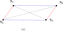
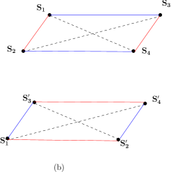
Figure 2: (a) (color online) The model of the four-spin system with the Yangian symmetry, the red line represents the exchange constant $a_{12}$, and the blue represent $a_{13}$. (b) (color online) The model of the extended {V6}-type molecule, the interaction between the two parallelograms is $H_{inter}=\Delta(\mathbf{S}_{A}\times\mathbf{S}_{A^{\prime}})_{y}$, which is totally similar to the {V6} molecule.

The eigenvalues and eigenstates of the Hamiltonian Eq. (3.1) are as follows:

$$H_{4}|\psi_{2,m}\rangle = E_{2,m}|\psi_{2,m}\rangle=(a_{12}+\frac{1}{2}a_{13})|\psi_{2,m}\rangle,$$

$$H_{4}|\psi^{1}_{1,m}\rangle = E_{1,m}^{1}|\psi^{1}_{1,m}\rangle=-\frac{1}{2}a_{13}|\psi^{1}_{1,m}\rangle,$$

$$H_{4}|\psi^{2}_{1,m}\rangle = E_{1,m}^{2}|\psi^{2}_{1,m}\rangle=(\frac{1}{3}a_{12}-\frac{5}{6}a_{13})|\psi^{2}_{1,m}\rangle,$$

$$H_{4}|\psi^{3}_{1,m}\rangle = E_{1,m}^{3}|\psi^{3}_{1,m}\rangle=(-\frac{4}{3}a_{12}+\frac{5}{6}a_{13})|\psi^{3}_{1,m}\rangle,$$

$$H_{4}|\psi^{+}_{0,0}\rangle = E_{0,0}^{+}|\psi^{+}_{0,0}\rangle=(-2a_{12}+\frac{1}{2}a_{13})|\psi^{+}_{0,0}\rangle,$$

$$H_{4}|\psi^{-}_{0,0}\rangle = E_{0,0}^{-}|\psi^{-}_{0,0}\rangle=-\frac{3}{2}a_{13}|\psi^{-}_{0,0}\rangle,$$ (18)

where $m$ is the quantum number of $S_{z}$ and the eigenstates are shown by Eq.(C) in the Appendix.C. If a magnetic field is applied, the states with different quantum numbers $m$ will split because of the Zeeman Effect. When the field is weak enough, we emphasize that the singlet state is not always the ground state. In fact, the ground state depends on the values of the exchange constants. By choosing some suitable constants, we can get the ground states with total spin $S=1$. For example, when $a_{12}>0,a_{13}<0$, and $a_{13}<-2a_{12}$, the energy levels are $E^{3}_{1,m}<E^{+}_{0,0}<E_{2,m}<E^{-}_{0,0}<E^{1}_{1,m}<E^{2}_{1,m}$, so the ground state is

$$|\psi^{3}_{1,-1}\rangle=\frac{1}{\sqrt{20}}\left(|\uparrow\downarrow\downarrow\downarrow\rangle-3|\downarrow\uparrow\downarrow\downarrow\rangle+3|\downarrow\downarrow\uparrow\downarrow\rangle-|\downarrow\downarrow\downarrow\uparrow\rangle\right).$$

Thus, we have got the Hamiltonian of the four-spin system determined by the Yangian symmetry. In a special case it is a model of parallelogram. It allows the ground state with $S=1$ instead of $S=0$. This is an interesting case not considered before, and we shall predict the “{V8}”-type molecule based on this result and make more theoretical predictions.

3.2 The magnetization of “{V8}”-type molecule

In the molecule {V6} we have shown that there is Yangian symmetry characterized by the operator $Q$ for each triangle. Meanwhile it has also been proved by the experiment[2] that there is a DM interaction between the two triangular pieces in {V6}. It causes the LZS transition.[6] The effect of the LZS transition can be reflected through the magnetization of the molecular {V6}.

It is natural to extend the LZS transition for {V6} to a molecular system comprised of two parallelograms. The molecular model is shown in Fig.2(b), which is called “{V8}”. We also assume that there is a similar DM interaction written as $H_{inter}=\Delta(\mathbf{S}_{A}\times\mathbf{S}_{A^{\prime}})_{y}$ between the two parallelograms. The operators $\mathbf{S}_{A}$ and $\mathbf{S}_{A^{\prime}}$ are the total spin operators of the two parallelograms, respectively. Obviously, it is complicated to calculate such a system with eight $\frac{1}{2}$-spins. To simplify the situation, we only consider the ground state of each parallelogram as in the molecule {V6}.[3] If the total spin of ground state is zero, it will make no sense to study the magnetization. However, if the total spin is one, we can make a prediction about its magnetization. Extending the approach working well for {V6} model the Hamiltonian of “{V8}” model will be written as:

$$\mathscr{H}=\hbar\gamma B(t)(S_{Az}+S_{A^{\prime}z})+\Delta(\mathbf{S}_{A}\times\mathbf{S}_{A^{\prime}})_{y},$$ (19)

where the spins $S_{A}=1$ and $S_{A^{\prime}}=1$, and $\gamma$ is the gyromagnetic ratio. The magnetic field $B(t)$ is along the $z$ axis and varies with the time. The first term in Eq.(19) is about the Zeeman Energy, and the second one is the special DM interaction leading to the LZS transition and is assumed to be tiny. By exactly diagonalizing the Hamiltonian $\mathscr{H}$, we can get the energy levels shown in Fig.3.

Figure 3: The scheme of the energy levels of the system comprised of two parallelograms with a DM interaction between them, where $\Delta$ is the energy gap of the Landau-Zener tunneling.

The DM interaction plays an important role only near the “crossing point” of the energy levels where the magnetic field is absent. Far away from the “crossing point”, the system behaves as two independent particles with each spin $S=1$, so we just need to consider one particle to investigate the magnetization of the system. In the experiment, the measurement of the magnetization is related to the relaxation time of the magnetization, and here we assume the relaxation time is long compared with the experimental time so that the hysteresis effect can be observed. The general method to investigate the magnetization has been well discussed in the Ref.[1], and we shall directly refer to the conclusion in the Ref.[1]. Using the standard formula (33) in Ref.[1]

$$\frac{d\rho_{NN}}{dt}=\sum_{N^{\prime}}W_{N^{\prime}N}\left(t\right)\rho_{N^{\prime}N^{\prime}}-\sum_{N^{\prime}}W_{NN^{\prime}}\left(t\right)\rho_{NN}$$

where the meaning of $\rho$ and $W$ will be seen clearly later, we obtain the equation of the magnetization dynamic for spin $S=1$

$$\frac{d}{dt}\left(\begin{array}[]{c}\frac{M}{-\hbar\gamma}\\ \rho_{00}\end{array}\right)=\left(\begin{array}[]{cc}C_{1}&C_{2}\\ C_{3}&C_{4}\end{array}\right)\left(\begin{array}[]{c}\frac{M}{-\hbar\gamma}\\ \rho_{00}\end{array}\right)+\left(\begin{array}[]{c}E\\ F\end{array}\right),$$ (28)

where $M$ is the magnetization of the system, and $\rho$ is the density operator. The magnetization is written as: $M=-\hbar\gamma\langle S_{z}\rangle=-\hbar\gamma(\rho_{++}-\rho_{--})$ and the coefficients in Eq.(28) are as follows:

$$C_{1} = -\frac{1}{2}(W_{-0}-W_{+0})-W_{-+}-W_{+-},$$

$$C_{2} = \frac{1}{2}(W_{+0}-W_{-0})+W_{0+}-W_{0-}+W_{+-}-W_{-+},$$

$$C_{3} = \frac{1}{2}(W_{+0}-W_{-0}),$$

$$C_{4} = -\frac{1}{2}(W_{+0}+W_{-0}+2W_{0+}+2W_{0-}),$$

$$E = \frac{1}{2}(W_{-0}-W_{+0})+W_{-+}-W_{+-},$$

$$F = \frac{1}{2}(W_{+0}+W_{-0}).$$

The quantity $W_{NN^{\prime}}$ represents the transition probability from the state $|N\rangle$ to $|N^{\prime}\rangle$, where $N$, $N^{\prime}$ is the magnetic quantum number characterized as $+,0,-$. If we take one-phonon process approximation the transition probability can be replaced by[9]

$$W_{NN^{\prime}}=\frac{A\delta^{3}}{1-e^{-\beta\hbar\delta}},$$

where $\delta=E_{N}-E_{N^{\prime}}=\hbar\gamma B(t)(N-N^{\prime})$ is the energy difference between two levels. When a pulsed magnetic field is applied, a hysteresis loop(see Fig.4) can be obtained from the Eq.(28), where the magnetization has been normalized with $M_{max}=\hbar\gamma$. All the parameters in the Eq.(28) have been taken the data provided in the Ref.[2] for {V6} molecule. We see that it is the usual hysteresis loop of a molecular magnet with the spin $S=1$.

However, the LZS transition must be considered when the magnetic field varies to the vicinity of the “crossing point” in the “{V8}” model. The total Hamiltonian is written as Eq.(19), and the off-diagonal elements can no longer be ignored. Diagonalizing Eq. (19) the exact energy levels read

$$E_{2,0} = E_{1,0}=E_{0,0}=0;$$

$$E_{2,\pm 1} = \pm\sqrt{B^{2}(t)+\Delta^{2}};$$

$$E_{2,\pm 2} = \pm\frac{1}{\sqrt{2}}\Bigg{[}5\mu^{2}B^{2}(t)+3\Delta^{2}+\sqrt{9\mu^{4}B^{4}(t)+30\mu^{2}B^{2}(t)+\Delta^{4}}\Bigg{]}^{\frac{1}{2}};$$

$$E_{1,\pm 1} = \pm\frac{1}{\sqrt{2}}\Bigg{[}5\mu^{2}B^{2}(t)+3\Delta^{2}-\sqrt{9\mu^{4}B^{4}(t)+30\mu^{2}B^{2}(t)+\Delta^{4}}\Bigg{]}^{\frac{1}{2}},$$

where the subscript $(l,m)$ corresponds to the state $|l,m\rangle$ which is the asymptotic eigenstates when the field is strong. Here $l$ is the quantum number of total spin, and $m$ is the magnetic quantum number. For simplicity, we just choose the nearest three levels $E_{2,-1},E_{2,0},E_{2,1}$ for a weak field to investigate the effect of the off-diagonal elements. These three levels can be viewed as the eigenvalues of the Hamiltonian with the matrix form

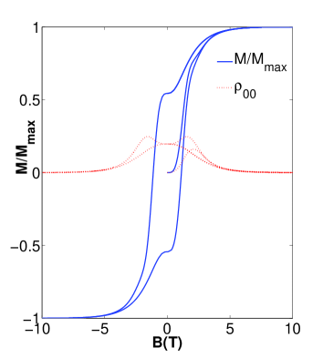
Figure 4: (color online) The magnetization of the four-spin system in a low temperature.The blue solid line is the magnetization, and the red dashed line is the density matrix $\rho_{00}$. The function of the magnetic field varies with the time as $B(t)=10\sin(t)$.

$$\mathscr{H}=\left(\begin{array}[]{ccc}B\left(t\right)&\frac{\Delta}{\sqrt{2}}&0\\ \frac{\Delta}{\sqrt{2}}&0&\frac{\Delta}{\sqrt{2}}\\ 0&\frac{\Delta}{\sqrt{2}}&-B\left(t\right)\end{array}\right),$$ (32)

whose eigenstates are

$$|E_{+},t\rangle = \left(\frac{1+\cos\beta}{2},\frac{\sin\beta}{\sqrt{2}},\frac{1-\cos\beta}{2}\right)^{T},$$

$$|E_{0},t\rangle = \left(\frac{-\sin\beta}{\sqrt{2}},\cos\beta,\frac{\sin\beta}{\sqrt{2}},\right)^{T},$$

$$|E_{-},t\rangle = \left(\frac{1-\cos\beta}{2},-\frac{\sin\beta}{\sqrt{2}},\frac{1+\cos\beta}{2},\right)^{T},$$ (33)

where the angle $\beta$ is determined by $\cos\beta=\frac{B\left(t\right)}{\sqrt{B^{2}\left(t\right)+\Delta^{2}}}$ and the corresponding eigenvalues are $E_{0}=0,\qquad E_{\pm}=\pm\sqrt{B^{2}\left(t\right)+\Delta^{2}}$. Following the method shown in Ref.[1] and assuming the Landau-Zener tunneling in adiabatic approximation, we derive the magnetization for spin $S=1$:

$$M=-\hbar\gamma\langle S_{z}\rangle=-\hbar\gamma\left(\tilde{\rho}_{++}S^{++}_{z}+\tilde{\rho}_{00}S^{00}_{z}+\tilde{\rho}_{--}S^{--}_{z}\right).$$ (34)

It is easy to calculate the matrix elements of $S_{z}$ ,and the Eq.(34) can be simplified as $M=\hbar\gamma\cos\beta\cdot n$. Here $n$ is defined as $n=\tilde{\rho}_{--}-\tilde{\rho}_{++}$, and obeys the same Bloch equation as Eq. (28):

$$\frac{d}{dt}\left(\begin{array}[]{c}n\left(t\right)\\ \tilde{\rho}_{00}\end{array}\right)=\left(\begin{array}[]{cc}C_{1}&C_{2}\\ C_{3}&C_{4}\end{array}\right)\left(\begin{array}[]{c}n\left(t\right)\\ \tilde{\rho}_{00}\end{array}\right)+\left(\begin{array}[]{c}E\\ F\end{array}\right).$$ (43)

Combining the Eq.(34) with Eq. (43), we can get the magnetization of the system as shown in Fig. 5, where the applied magnetic field is taken as $B(t)=10\sin(t)$ varying in a period $t\in[0,\pi]$. Similar to the {V6} molecule the magnetization can be probed because of the LZS effect.

In a summary, we extended the properties of the molecule {V6} to a “{V8}”-type molecule comprised of two parallelograms. By investigating its magnetization of the molecular model, we draw the conclusion that the “{V8}”-type molecule behaves similar to the molecule {V6}.

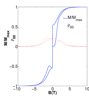
Figure 5: (color online) The magnetization of the system “{V8}” comprised of two parallelograms with DM interaction between them. The blue solid line is the magnetization, and the red dashed line is the density matrix $\rho_{00}$. It turns out that the density matrix $\rho_{00}$ is not affected by the off-diagonal matrix of the Hamiltonian, and its magnetization has a similar behavior to the molecular {V6}.[10]

4 The local spin moments configuration of the four-spin system

In this section, we will make up another molecule whose model can be treated as one parallelogram and give a prediction about its local spin moments configuration.

To make up the theoretical molecular model, we need recall the model of {V15} which can be considered as an isosceles triangle in a low temperature first. The molecule {V15} is comprised of 15 $V^{4+}$ ions with each spin $s=1/2$, and the ions are arranged in a quasispherical layered structure with a triangle sandwiched between two hexagons as is shown in the Fig.6(a). Each hexagon of {V15} consists of three pairs of strongly coupled spins with $J_{1}\sim 800K$.[11] Each spin of the $V^{4+}$ ions in the central triangle is coupled with the spins in both hexagons with $J_{2}=150K$ and $J_{3}=300K$, resulting in a very weak exchange interaction between the spins within the central triangle with $J_{0}=2.44K$.[11, 12] When the temperature is low enough, the molecule {V15} has a much simpler approximation: the two hexagons can be omitted because each total spin is zero, and the only survived part is just a simple Heisenberg spin triangle.[13] It has been revealed that such a Heisenberg spin triangle model is isosceles with the relationship $J_{13}>J_{12}=J_{23}$ by measuring the local spin moments configuration in an NMR experiment.[4] So the Yangian symmetry also exists in the {V15} molecule in a low temperature, and it can be detected by measuring the local spin moments configuration.

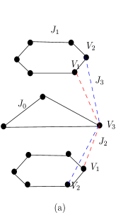
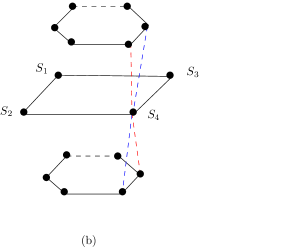
Figure 6: (a)(color online) The structure model of the molecular {V15}. The solid circles represent the $V^{4+}$($s=1/2$) ions. In a low temperature, only the triangle in the middle is considered. (b)(color online) The theoretical molecule whose model is a parallelogram satisfying the condition Eq.(3.1). The upper and lower polygons are comprised of 2N particles so that their total spins in the ground state is zero in the low temperature respectively. The different colors represent the different coupling constants.

Next we shall extend such a molecular model to the four-spin system and give the prediction regarding the local spin moments configuration. The assumed molecule is shown in the Fig.6(b) whose structure is totally similar to the {V15} molecule. The numbers of the ions in the upper and the lower polygons are both even. And they are coupled to the special parallelogram in the middle, which results in some special exchange constants in the middle parallelogram satisfying the Eq.(3.1). Similar to the {V15} molecule, such a molecule can be viewed as a single parallelogram described in Sec.3. We can calculate the local spin moments configuration of this model in the NMR experiment. The local spin moment is usually written as $\mu_{i}=-g\mu_{B}\langle\phi_{g}|S^{3}_{i}|\phi_{g}\rangle$, where the operator $S^{3}_{i}$ $(i=1,2,3,4)$ is the $z$-component of the spin operator of the $i$-th particle, $g=2$, and $\mu_{B}$ is the Bohr magneton. The state $|\phi_{g}\rangle$ is the ground state of the system. Through direct calculation, we can obtain the local moments of the four particles. It is highly nontrivial that the ground state of a four-spin system is with $S=1$, so we mainly focus on such a case and predict its measurement in the experiment. When the exchange constants satisfy the relationship $a_{12}>0,a_{13}<0,a_{13}<-2a_{12}$, the ground state is $\psi^{3}_{1,-1}$, and the corresponding local spin moments are $\frac{9}{10}\mu_{B},\frac{1}{10}\mu_{B},\frac{1}{10}\mu_{B},\frac{9}{10}\mu_{B}$,respectively. So the observations are $\frac{1}{10}\mu_{B},\frac{9}{10}\mu_{B}$ when the NMR experiment is performed. In this way, we can tell whether there is the Yangian symmetry by measuring its local spin moments.

5 Summary

By investigating the experimental results on the molecular {V6}, we introduce a special form of the DM interaction operator, i.e. Yangian operator to describe the symmetry of the molecule. Meanwhile we extend the symmetry operator to the four-spin system. We find that the ground state may be no longer the singlet state in a four-spin system determined by the Yangian symmetry. By choosing suitable interaction constants, the state with spin $S=1$ can be the ground state. When the ground state is with spin $S=1$, we extend the DM interaction in the {V6} molecule to our new model “{V8}”. By investigating its magnetization, we find that it behaves similar to the {V6} molecule. At last, we propose another theoretical molecular model and make a prediction regarding its local spin moments configuration which might be measured by the NMR experiment in principle.

Appendix A The mathematics of Yangian

Yangian algebras were established by Drinfel’d.[15, 16, 17] A Yangian is formed by a set $\{\mathbf{I},\mathbf{Y}\}$ obeying the commutation relations:

$$[I_{\lambda},I_{\mu}]=c_{\lambda\mu\nu}I_{\nu},\qquad[I_{\lambda},Y_{\mu}]=c_{\lambda\mu\nu}Y_{\nu},$$ (A1)

$$[[Y_{\lambda},[Y_{\mu},I_{\nu}]]-[I_{\lambda},[Y_{\mu},Y_{\nu}]]=\lambda a_{\lambda\mu\nu\alpha\beta\gamma}\{I_{\alpha},I_{\beta},I_{\gamma}\},$$ (A2)

$$[[Y_{\lambda},Y_{\mu}],[I_{\sigma},Y_{\tau\tauup}]]+[[Y_{\sigma},Y_{\tauup}],[I_{\lambda},Y_{\mu}]]$$

$$=\lambda(a_{\lambda\mu\nu\alpha\beta\gamma}c_{\sigma\tauup\nu}+a_{\sigma\tauup\nu\alpha\beta\gamma}c_{\lambda\mu\nu})\{I_{\alpha},I_{\beta},Y_{\gamma}\},$$ (A3)

where the set of $I_{\lambda}$ forms a simple Lie algebra characterized by $c_{\lambda\mu\nu}$ and the repeated indices mean summation. The definitions of $a_{\lambda\mu\nu\alpha\beta\gamma}$ and $\{x_{i},x_{j},x_{k}\}$ were given in the Ref.[15],

$$a_{\lambda\mu\nu\alpha\beta\gamma} = \frac{1}{4!}c_{\lambda\alpha\sigma}c_{\mu\beta\tauup}c_{\nu\gamma\rho}c_{\sigma\tauup\rho},$$ (A4)

$$\{x_{1},x_{2},x_{3}\} = \sum_{i\neq j\neq k}x_{i}x_{j}x_{k}.$$ (A5)

In the present model

$$c_{\lambda\mu\nu}=i\epsilon_{\lambda\mu\nu}\quad(\lambda,\mu,\nu=1,2,3)$$ (A6)

where $\epsilon_{\lambda\mu\nu}$ is the total anti-symmetric tensor. It turns out that Eq. (A2) is automatically satisfied. We then should simplify the Eq. (A3). Substituting Eq.(A6) into Eq.(A3) and considering all the possibilities of values of $\lambda,\mu,\nu,...$ the Eq.(A3) reduces to

$$[J_{+},[J_{3},J_{+}]] = \frac{\lambda}{4}I_{+}(J_{+}I_{3}-I_{+}J_{3}),$$ (A7)

$${}[J_{-},[J_{3},J_{-}]] = \frac{\lambda}{4}I_{-}(J_{-}I_{3}-I_{-}J_{3}).$$ (A8)

and

$$[J_{\pm},[J_{+},J_{-}]]+2[J_{3},[J_{3},J_{\pm}]]=\lambda\{2I_{3}(J_{\pm}I_{3}-I_{\pm}J_{3})+I_{\pm}(I_{\pm}J_{\mp}-J_{\pm}I_{\mp})\}$$ (A9)

where $J_{\pm}=J_{1}\pm iJ_{2},\quad I_{\pm}=I_{1}\pm iI_{2}$.
It should be noted that

$$J_{\mp}I\pm-I_{\mp}J_{\pm}=I_{\pm}J_{\mp}-J_{\pm}I_{\mp}.$$ (A10)

We can prove that based on the Jacobian identities Eq. (A9) is satisfied. Therefore only Eq. (A1) and either (A7) or (A8) are independent. The similar relations for SU(3) and SO(5) occur. Their forms are complicated , so we shall not explain them here. In the system comprised of $n$ particles, if the operator $\mathbf{I}$ is taken as the total spin operator $\mathbf{I}=\sum^{n}_{i=1}\mathbf{S}_{i}$, the Yangian operator $\mathbf{Y}$ can be realized in terms of

$$\mathbf{Y}=\sum^{n}_{i=1}u_{i}\mathbf{S}_{i}+i\sum^{n}_{i<j}(\mathbf{S}_{i}\times\mathbf{S}_{j}),$$ (A11)

where $u_{i}$ can be arbitrary parameters and $\mathbf{S}_{i}$ is the spin of the $i$-th particle. It can be verified that the operators $\mathbf{I}$ and $\mathbf{Y}$ satisfy the Eq.(A1), Eq.(A2) and Eq.(A3), i.e. they form a Yangian. A set $\{Q=Y^{2},I^{2},I_{3}\}$ forms commuting set, so we use $Q$, $I^{2}$ and $I_{3}$ characterize a system. If $[[Q,H]]=0$, the Hamiltonian and $Q$ share the same eigenvalues. The Hamiltonian of Heisenberg model for $n$-spin system is usually written as:

$$H=\sum^{n}_{i<j}a_{ij}\mathbf{S}_{i}\cdot\mathbf{S}_{j},$$ (A12)

where $a_{ij}$ is the exchange constant between the $i$-th particle and $j$-th particle. In contrast to the spin chain models we focus on few-body problem, say $n=3$ ({V6}) and $n=4$ (theoretical “{V8}” model). It is emphasized that the realization of Yangian shown by Eq. (A11) is not unique. There are other realization of Eq.(A1), Eq.(A2) and Eq.(A3), but Eq. (A11) is suitable to our discussion.

Appendix B Three-spin system with the Yangian symmetry

For a three-spin system the Yangian operator $\mathbf{Y}$ is taken as Eq.(A11), and in the Hamiltonian Eq.(A12) we have $n=3$. We need to calculate the eigenvalues and eigenstates of $Q$. The square of $\mathbf{Y}$ is given by

$$Q = \sum^{3}_{i=1}u^{2}_{i}S^{2}_{i}+2(u_{1}u_{2}\mathbf{S_{1}}\cdot\mathbf{S_{2}}+u_{2}u_{3}\mathbf{S_{2}}\cdot\mathbf{S_{3}}+u_{1}u_{3}\mathbf{S_{1}}\cdot\mathbf{S_{3}})$$

$$+2i(u_{1}-u_{2}+u_{3})\mathbf{S_{1}}\cdot(\mathbf{S_{2}}\times\mathbf{S_{3}})-\{S^{2}_{1}S^{2}_{2}+S^{2}_{2}S^{2}_{3}+S^{2}_{1}S^{2}_{3}$$

$$-(\mathbf{S_{1}}\cdot\mathbf{S_{2}}+\mathbf{S_{2}}\cdot\mathbf{S_{3}}+\mathbf{S_{1}}\cdot\mathbf{S_{3}})+2S^{2}_{1}(\mathbf{S_{2}}\cdot\mathbf{S_{3}})+2S^{2}_{3}(\mathbf{S_{1}}\cdot\mathbf{S_{2}})$$

$$-2S^{2}_{2}(\mathbf{S_{1}}\cdot\mathbf{S_{3}})-(\mathbf{S_{1}}\cdot\mathbf{S_{2}}+\mathbf{S_{2}}\cdot\mathbf{S_{3}}+\mathbf{S_{1}}\cdot\mathbf{S_{3}})^{2}$$

$$+2[(\mathbf{S_{1}}\cdot\mathbf{S_{2}})(\mathbf{S_{2}}\cdot\mathbf{S_{3}})+(\mathbf{S_{2}}\cdot\mathbf{S_{3}})(\mathbf{S_{1}}\cdot\mathbf{S_{2}})]\}$$

And the usual Lie algebraic bases for three $\frac{1}{2}$-spins are as follows:

$$|\phi_{\frac{3}{2},-\frac{3}{2}}\rangle = |\downarrow\downarrow\downarrow\rangle,$$

$$|\phi_{\frac{3}{2},-\frac{1}{2}}\rangle = \frac{1}{\sqrt{3}}(|\uparrow\downarrow\downarrow\rangle+|\downarrow\uparrow\downarrow\rangle+|\downarrow\downarrow\uparrow\rangle),$$

$$|\phi_{\frac{3}{2},\frac{1}{2}}\rangle = \frac{1}{\sqrt{3}}(|\uparrow\uparrow\downarrow\rangle+|\uparrow\downarrow\uparrow\rangle+|\downarrow\uparrow\uparrow\rangle),$$

$$|\phi_{\frac{3}{2},\frac{3}{2}}\rangle = |\uparrow\uparrow\uparrow\rangle,$$

$$|\phi^{\prime}_{\frac{1}{2},\frac{1}{2}}\rangle = \frac{1}{\sqrt{6}}(|\downarrow\uparrow\uparrow\rangle+|\uparrow\downarrow\uparrow\rangle-2|\uparrow\uparrow\downarrow\rangle),$$

$$|\phi^{\prime}_{\frac{1}{2},-\frac{1}{2}}\rangle = \frac{1}{\sqrt{6}}(|\uparrow\downarrow\downarrow\rangle+|\downarrow\uparrow\downarrow\rangle-2|\downarrow\downarrow\uparrow\rangle),$$

$$|\phi_{\frac{1}{2},\frac{1}{2}}\rangle = \frac{1}{\sqrt{2}}(|\downarrow\uparrow\uparrow\rangle+|\uparrow\downarrow\uparrow\rangle),$$

$$|\phi_{\frac{1}{2},-\frac{1}{2}}\rangle = \frac{1}{\sqrt{2}}(|\uparrow\downarrow\downarrow\rangle+|\downarrow\uparrow\downarrow\rangle).$$

It can be easily verified that:

$$Q|\phi_{\frac{3}{2},m}\rangle = [\frac{3}{4}(u^{2}_{1}+u^{2}_{2}+u^{2}_{3})+\frac{1}{2}(u_{1}u_{2}+u_{2}u_{3}+u_{1}u_{3})-1]|\phi_{\frac{3}{2},m}\rangle,$$

$$Q|\phi^{\prime}_{\frac{1}{2},m}\rangle = [\frac{3}{4}(u^{2}_{1}+u^{2}_{2}+u^{2}_{3})+\frac{1}{2}u_{1}u_{2}-u_{2}u_{3}-u_{1}u_{3}-\frac{7}{4}]|\phi^{\prime}_{\frac{1}{2},m}\rangle$$

$$-\frac{\sqrt{3}}{2}(u_{1}-u_{2}+1)(u_{3}+1)|\phi_{\frac{1}{2},m}\rangle,$$

$$Q|\phi_{\frac{1}{2},m}\rangle = -\frac{\sqrt{3}}{2}(u_{1}-u_{2}-1)(u_{3}-1)|\phi^{\prime}_{\frac{1}{2},m}\rangle+[\frac{3}{4}(u_{1}-u_{2})^{2}+\frac{3}{4}u^{2}_{3}-\frac{3}{4}]|\phi^{\prime}_{\frac{1}{2},m}\rangle.$$

We would like to note the difference between Lie algebra and Yangian in diagonalizing process. Suppose a Hamiltonian, in general, the eigenfunction of $H$ is written as $|\psi\rangle=\sum_{I}c_{I}|\psi_{I}\rangle$ where $|\psi_{I}\rangle$ is the eigenfunction of $I^{2}$. However, if $[H,\mathbf{Y}]=0$, both $H$ and $\mathbf{Y}$ share the same wave function, because $\mathbf{Y}$ is an operator acting on tensor space which is much larger than Lie algebra space. For this reason, for symmetric $a_{ij}$ in Eq. (A12) we choose symmetric $Q$ which leads to $u_{2}=u_{1}+u_{3}$. If $u_{1}=u_{2}=u_{3}=0$, the Yangian operator reduces to the special form fo the DM interaction operator Eq. (2). In this special case, we can easily obtain the eigenvalues and the eigenvectors of $Q$ as:

$$Q|\phi_{\frac{3}{2},m}\rangle=-1|\phi_{\frac{3}{2},m}\rangle,$$

$$Q|\psi^{\alpha}_{\frac{1}{2},m}\rangle=-\frac{1}{4}|\psi^{\alpha}_{\frac{1}{2},m}\rangle,$$

$$Q|\psi^{beta}_{\frac{1}{2},m}\rangle=-\frac{9}{4}|\psi^{\beta}_{\frac{1}{2},m}\rangle,$$

where $m$ is the magnetic quantum number, and the eigenvectors are

$$|\psi^{\alpha}_{\frac{1}{2},m}\rangle = -\frac{1}{2}|\phi^{\prime}_{\frac{1}{2},m}\rangle+\frac{\sqrt{3}}{2}|\phi_{\frac{1}{2},m}\rangle,$$

$$|\psi^{\beta}_{\frac{1}{2},m}\rangle = -\frac{\sqrt{3}}{2}|\phi^{\prime}_{\frac{1}{2},m}\rangle+\frac{1}{2}|\phi_{\frac{1}{2},m}\rangle.$$

When $m=-1/2$ the two states with total spin $S=1/2$ are reduced to the Eq.(5) and Eq.(6). We can see that the operator $Q$ just mixes the states with the same numbers of $S^{2},S_{z}$. To let $Q$ and the Hamiltonian share the same eigenstates i.e.

$$H|\phi_{\frac{3}{2},m}\rangle = E_{\frac{3}{2},m}|\phi_{\frac{3}{2},m}\rangle,$$

$$H|\psi^{\alpha}_{\frac{1}{2},m}\rangle = E^{\alpha}_{\frac{1}{2},m}|\psi^{\alpha}_{\frac{1}{2},m}\rangle,$$

$$H|\psi^{\beta}_{\frac{1}{2},m}\rangle = E^{\beta}_{\frac{1}{2},m}|\psi^{\beta}_{\frac{1}{2},m}\rangle$$

by direct calculation, we get the relationship $a_{12}=a_{23}$ in the Hamiltonian(A12) and the corresponding energy levels $E_{\frac{1}{2},-\frac{1}{2}}^{\alpha}=\frac{1}{4}J_{13}-J_{12}$, $E_{\frac{1}{2},-\frac{1}{2}}^{\beta}=-\frac{3}{4}J_{13}$, $E_{\frac{3}{2},-\frac{3}{2}}=\frac{J_{12}}{2}+\frac{J_{13}}{4}$.

Appendix C The four-spin system with the Yangian symmetry

For a system comprised of four $\frac{1}{2}$-spins, the similar process for $n=4$ will be performed. In the Yangian operator Eq.(A11) and the Hamiltonian Eq.(A12) we take $n=4$. The operator $Q$ in them is

$$Q = \sum^{4}_{i=1}u^{2}_{i}S^{2}_{i}+2\sum_{i,j(i<j)}^{4}u_{i}u_{j}\mathbf{S_{i}}\cdot\mathbf{S_{j}}$$

$$+2i[(u_{1}-u_{2}+u_{3})\mathbf{S_{1}}\cdot(\mathbf{S_{2}}\times\mathbf{S_{3}})+(u_{1}-u_{2}+u_{4})\mathbf{S_{1}}\cdot(\mathbf{S_{2}}\times\mathbf{S_{4}})$$

$$+(u_{1}-u_{3}+u_{4})\mathbf{S_{1}}\cdot(\mathbf{S_{3}}\times\mathbf{S_{4}})+(u_{2}-u_{3}+u_{4})\mathbf{S_{2}}\cdot(\mathbf{S_{3}}\times\mathbf{S_{4}})]$$

$$-\{\sum_{i,j(i<j)}^{4}S^{2}_{i}S^{2}_{j}-[\sum_{i,j(i<j)}^{4}(\mathbf{S_{i}}\cdot\mathbf{S_{j}})]^{2}-\sum_{i,j(i<j)}^{4}(\mathbf{S_{i}}\cdot\mathbf{S_{j}})$$

$$+2[S_{1}^{2}(\mathbf{S_{2}}\cdot\mathbf{S_{3}}+\mathbf{S_{2}}\cdot\mathbf{S_{4}}+\mathbf{S_{3}}\cdot\mathbf{S_{4}})+S^{2}_{2}(\mathbf{S_{3}}\cdot\mathbf{S_{4}}-\mathbf{S_{1}}\cdot\mathbf{S_{3}}$$

$$-\mathbf{S_{1}}\cdot\mathbf{S_{4}})+S^{2}_{3}(\mathbf{S_{1}}\cdot\mathbf{S_{2}}-\mathbf{S_{1}}\cdot\mathbf{S_{4}}-\mathbf{S_{2}}\cdot\mathbf{S_{4}})$$

$$+S^{2}_{4}(\mathbf{S_{1}}\cdot\mathbf{S_{2}}+\mathbf{S_{1}}\cdot\mathbf{S_{3}}+\mathbf{S_{2}}\cdot\mathbf{S_{3}})]$$

$$+2[(\mathbf{S_{2}}\cdot\mathbf{S_{3}})(\mathbf{S_{1}}\cdot\mathbf{S_{2}})+(\mathbf{S_{1}}\cdot\mathbf{S_{2}})(\mathbf{S_{2}}\cdot\mathbf{S_{3}})]$$

$$+2[(\mathbf{S_{2}}\cdot\mathbf{S_{4}})(\mathbf{S_{1}}\cdot\mathbf{S_{2}})+(\mathbf{S_{1}}\cdot\mathbf{S_{2}})(\mathbf{S_{2}}\cdot\mathbf{S_{4}})]$$

$$+2[(\mathbf{S_{3}}\cdot\mathbf{S_{4}})(\mathbf{S_{1}}\cdot\mathbf{S_{3}})+(\mathbf{S_{1}}\cdot\mathbf{S_{3}})(\mathbf{S_{3}}\cdot\mathbf{S_{4}})]$$

$$+2[(\mathbf{S_{3}}\cdot\mathbf{S_{4}})(\mathbf{S_{2}}\cdot\mathbf{S_{3}})+(\mathbf{S_{2}}\cdot\mathbf{S_{3}})(\mathbf{S_{3}}\cdot\mathbf{S_{4}})]$$

$$+2[(\mathbf{S_{1}}\cdot\mathbf{S_{3}})(\mathbf{S_{2}}\cdot\mathbf{S_{4}})-(\mathbf{S_{1}}\cdot\mathbf{S_{4}})(\mathbf{S_{2}}\cdot\mathbf{S_{3}})+3(\mathbf{S_{1}}\cdot\mathbf{S_{2}})(\mathbf{S_{3}}\cdot\mathbf{S_{4}})]\}$$

The usual Lie algebraic bases are standard:

$$|\phi_{2,-2}\rangle = |\downarrow\downarrow\downarrow\rangle,$$

$$|\phi_{2,-1}\rangle = \frac{1}{2}(|\uparrow\downarrow\downarrow\downarrow\rangle+|\downarrow\uparrow\downarrow\downarrow\rangle+|\downarrow\downarrow\uparrow\downarrow\rangle+\downarrow\downarrow\downarrow\uparrow\rangle),$$

$$|\phi_{2,0}\rangle = \frac{1}{\sqrt{6}}(|\uparrow\uparrow\downarrow\downarrow\rangle+\uparrow\downarrow\uparrow\downarrow\rangle+\uparrow\downarrow\downarrow\uparrow\rangle+\downarrow\uparrow\downarrow\uparrow\rangle+\downarrow\downarrow\uparrow\uparrow\rangle+\downarrow\uparrow\uparrow\downarrow\rangle),$$

$$|\phi_{2,1}\rangle = \frac{1}{2}(|\uparrow\uparrow\downarrow\uparrow\rangle+|\uparrow\downarrow\uparrow\uparrow\rangle+|\downarrow\uparrow\uparrow\uparrow\rangle+\uparrow\uparrow\uparrow\downarrow\rangle),$$

$$|\phi_{2,2}\rangle = |\uparrow\uparrow\uparrow\uparrow\rangle,$$

$$|\phi^{1}_{1,1}\rangle = \frac{1}{2}(-|\uparrow\uparrow\uparrow\downarrow\rangle+|\uparrow\uparrow\downarrow\uparrow\rangle-|\uparrow\downarrow\uparrow\uparrow\rangle-|\downarrow\uparrow\uparrow\uparrow\rangle),$$

$$|\phi^{1}_{1,0}\rangle = \frac{1}{\sqrt{2}}(|\uparrow\uparrow\downarrow\downarrow\rangle-|\downarrow\downarrow\uparrow\uparrow\rangle),$$

$$|\phi^{1}_{1,-1}\rangle = \frac{1}{2}(|\uparrow\downarrow\downarrow\downarrow\rangle+|\downarrow\uparrow\downarrow\downarrow\rangle-|\downarrow\downarrow\uparrow\downarrow\rangle-|\downarrow\downarrow\downarrow\uparrow\rangle-),$$

$$|\phi^{2}_{1,1}\rangle = \frac{1}{\sqrt{2}}(|\uparrow\downarrow\uparrow\uparrow\rangle-|\downarrow\uparrow\uparrow\uparrow\rangle),$$

$$|\phi^{2}_{1,0}\rangle = \frac{1}{2}(|\uparrow\downarrow\uparrow\downarrow\rangle+|\uparrow\downarrow\downarrow\uparrow\rangle-|\downarrow\uparrow\downarrow\uparrow\rangle-|\downarrow\uparrow\uparrow\downarrow\rangle),$$

$$|\phi^{2}_{1,-1}\rangle = \frac{1}{\sqrt{2}}(|\uparrow\downarrow\downarrow\downarrow\rangle-|\downarrow\uparrow\downarrow\downarrow\rangle),$$

$$|\phi^{3}_{1,1}\rangle = \frac{1}{\sqrt{2}}(|\uparrow\uparrow\uparrow\downarrow\rangle-|\uparrow\uparrow\downarrow\uparrow\rangle),$$

$$|\phi^{3}_{1,0}\rangle = \frac{1}{2}(|\uparrow\downarrow\uparrow\downarrow\rangle+|\downarrow\uparrow\uparrow\downarrow\rangle-|\downarrow\uparrow\downarrow\uparrow\rangle-|\uparrow\downarrow\downarrow\uparrow\rangle),$$

$$|\phi^{3}_{1,-1}\rangle = \frac{1}{\sqrt{2}}(|\downarrow\downarrow\uparrow\downarrow\rangle-|\downarrow\downarrow\downarrow\uparrow\rangle),$$

$$|\phi^{1}_{0,0}\rangle = \frac{1}{2\sqrt{3}}[2(|\uparrow\uparrow\downarrow\downarrow\rangle+|\downarrow\downarrow\uparrow\uparrow\rangle)-(|\uparrow\downarrow\uparrow\downarrow\rangle$$

$$+|\downarrow\uparrow\downarrow\uparrow\rangle+|\uparrow\downarrow\downarrow\uparrow\rangle+|\downarrow\uparrow\uparrow\downarrow\rangle)],$$

$$|\phi^{2}_{0,0}\rangle = \frac{1}{2}(|\uparrow\downarrow\uparrow\downarrow\rangle+|\downarrow\uparrow\downarrow\uparrow\rangle-|\uparrow\downarrow\downarrow\uparrow\rangle-|\downarrow\uparrow\uparrow\downarrow\rangle).$$

Then the action of $Q$ turns out that

$$Q|\phi_{2,m}\rangle = [\frac{3}{8}(u_{1}+u_{2}+u_{3}+u_{4})^{2}+\frac{1}{4}(u_{1}-u_{2})^{2}-\frac{5}{2}$$

$$+\frac{1}{8}(u_{1}+u_{2}-u_{3}-u_{4})^{2}+\frac{1}{4}(u_{3}-u_{4})^{2}]|\phi_{2,m}\rangle;$$

$$Q|\phi^{1}_{1,m}\rangle = [\frac{1}{2}(u^{2}_{1}+u^{2}_{2}+u^{2}_{3}+u^{2}_{4})-\frac{9}{2}+\frac{1}{4}(u_{1}+u_{2}-u_{3}-u_{4})^{2}]|\phi^{1}_{1,m}\rangle$$

$$-\frac{1}{\sqrt{2}}(u{1}-u_{2}+1)(u_{3}+u_{4}+2)|\phi^{2}_{1,m}\rangle+\frac{1}{\sqrt{2}}(u_{3}-u_{4}+1)(u_{1}-u_{2}-2)|\phi^{3}_{1,m}\rangle;$$

$$Q|\phi^{2}_{1,m}\rangle = -\frac{1}{\sqrt{2}}(u{1}-u_{2}+1)(u_{3}+u_{4}+2)|\phi^{1}_{1,m}\rangle+[\frac{1}{2}(u_{3}+u_{4})^{2}+\frac{1}{4}(u_{3}-u_{4})^{2}$$

$${}+\frac{3}{4}(u_{1}-u_{2})^{2}-1]|\phi^{2}_{1,m}\rangle+\frac{1}{2}(u_{1}-u_{2}-1)(u_{3}-u_{4}+1)|\phi^{3}_{1,m}\rangle;$$

$$Q|\phi^{3}_{1,m}\rangle = \frac{1}{\sqrt{2}}(u_{3}-u_{4}+1)(u_{1}-u_{2}-2)|\phi^{1}_{1,m}\rangle+\frac{1}{2}(u_{1}-u_{2}-1)(u_{3}-u_{4}+1)|\phi^{2}_{1,m}\rangle$$

$$+[\frac{1}{2}(u_{1}+u_{2})^{2}+\frac{1}{4}(u_{1}-u_{2})^{2}+\frac{3}{4}(u_{3}-u_{4})^{2}-1]|\phi^{3}_{1,m}\rangle;$$

$$Q|\phi^{1}_{0,0}\rangle = \{\frac{1}{2}(u_{1}+u_{2}-u_{3}-u_{4}-2)(u_{1}+u_{2}-u_{3}-u_{4}+2)+\frac{1}{4}[(u_{1}-u_{2})^{2}+(u_{3}-u_{4})^{2}-2]\}|\phi^{1}_{0,0}\rangle$$

$$-\frac{\sqrt{3}}{2}(u_{1}-u_{2}+1)(u_{3}-u_{4}+1)|\phi^{2}_{0,0}\rangle;$$

$$Q|\phi^{2}_{0,0}\rangle = -\frac{\sqrt{3}}{2}(u_{1}-u_{2}+1)(u_{3}-u_{4}+1)|\phi^{1}_{0,0}\rangle+\frac{3}{4}[(u_{1}-u_{2})^{2}+(u_{3}-u_{4})^{2}-2]|\phi^{2}_{0,0}\rangle;$$

where $m$ is the magnetic quantum number. However, a symmetric $Q$ requires $u_{1}=u_{2}=u_{3}=u_{4}=0$. So the first term of the Eq.(A11) must vanish, and the the Yangian operator is identified with special form of the DM interaction operator. In terms of Eq. (C.3) the eigenvalues and the eigenstates of the $Q$ are:

$$Q\left(\begin{array}[]{c}\phi_{2,m}\\ \psi^{1}_{1,m}\\ \psi^{2}_{1,m}\\ \psi^{3}_{1,m}\\ \psi^{+}_{00}\\ \psi^{-}_{00}\end{array}\right)=\left(\begin{array}[]{cccccc}-\frac{5}{2}&0&0&0&0&0\\ 0&-\frac{1}{2}&0&0&0&0\\ 0&0&-\frac{11}{2}&0&0&0\\ 0&0&0&-\frac{1}{2}&0&0\\ 0&0&0&0&-1&0\\ 0&0&0&0&0&-3\end{array}\right)\left(\begin{array}[]{c}\phi_{2,m}\\ \psi^{1}_{1,m}\\ \psi^{2}_{1,m}\\ \psi^{3}_{1,m}\\ \psi^{+}_{00}\\ \psi^{-}_{00}\end{array}\right),$$ (C22)

where the eigenstates are

$$|\psi_{2,m}\rangle = |\phi_{2,m}\rangle,$$

$$|\psi^{1}_{1,m}\rangle = \frac{2\sqrt{2}}{10}|\phi^{1}_{1,m}\rangle+\frac{1}{\sqrt{10}}|\phi^{2}_{1,m}\rangle+\frac{1}{\sqrt{10}}|\phi^{3}_{1,m}\rangle$$

$$|\psi^{2}_{1,m}\rangle = \frac{1}{\sqrt{2}}|\phi^{2}_{1,m}\rangle-\frac{1}{\sqrt{2}}|\phi^{3}_{1,m}\rangle$$

$$|\psi^{3}_{1,m}\rangle = -\frac{1}{\sqrt{5}}|\phi^{1}_{1,m}\rangle+\frac{2}{\sqrt{10}}|\phi^{2}_{1,m}\rangle+\frac{2}{\sqrt{10}}|\phi^{3}_{1,m}\rangle$$

$$|\psi^{+}_{0,0}\rangle = \frac{\sqrt{3}}{2}|\phi^{1}_{0,0}\rangle+\frac{1}{2}|\phi^{2}_{0,0}\rangle,$$

$$|\psi^{-}_{0,0}\rangle = -\frac{1}{2}|\phi^{1}_{0,0}\rangle+\frac{\sqrt{3}}{2}|\phi^{2}_{0,0}\rangle,$$

In detail, the eigenstates with some definite magnetic quantum number $m$ is expanded as follows:

$$|\phi_{2,-2}\rangle = |\downarrow\downarrow\downarrow\downarrow\rangle,$$

$$|\psi^{1}_{1,-1}\rangle = \frac{1}{2}\left(-|\uparrow\downarrow\downarrow\downarrow\rangle+|\downarrow\uparrow\downarrow\downarrow\rangle+|\downarrow\downarrow\uparrow\downarrow\rangle-|\downarrow\downarrow\downarrow\uparrow\rangle\right),$$

$$|\psi^{2}_{1,-1}\rangle = \frac{1}{\sqrt{20}}\left(3|\uparrow\downarrow\downarrow\downarrow\rangle+|\downarrow\uparrow\downarrow\downarrow\rangle-|\downarrow\downarrow\uparrow\downarrow\rangle-3|\downarrow\downarrow\downarrow\uparrow\rangle\right),$$

$$|\psi^{3}_{1,-1}\rangle = \frac{1}{\sqrt{20}}\left(|\uparrow\downarrow\downarrow\downarrow\rangle-3|\downarrow\uparrow\downarrow\downarrow\rangle+3|\downarrow\downarrow\uparrow\downarrow\rangle-|\downarrow\downarrow\downarrow\uparrow\rangle\right),$$

$$|\psi^{+}_{0,0}\rangle = \frac{1}{2\sqrt{3}}[\left(|\uparrow\uparrow\downarrow\downarrow\rangle+|\downarrow\downarrow\uparrow\uparrow\rangle\right)-2(|\uparrow\downarrow\uparrow\downarrow\rangle,$$

$$+|\downarrow\uparrow\downarrow\uparrow\rangle)+\left(|\uparrow\downarrow\downarrow\uparrow\rangle+|\downarrow\uparrow\uparrow\downarrow\rangle\right)],$$

$$|\psi^{-}_{0,0}\rangle = \frac{1}{2}[-\left(|\uparrow\uparrow\downarrow\downarrow\rangle+|\downarrow\downarrow\uparrow\uparrow\rangle\right)+\left(|\uparrow\downarrow\downarrow\uparrow\rangle+|\downarrow\uparrow\uparrow\downarrow\rangle\right)].$$

From Eq. (C22) it follows that for $S=1$ the two states for $Q=-\frac{1}{2}$ are degenerate. Hence, we need another variable $\theta$ to distinguish from each other:

$$|\psi^{1^{\prime}}_{1,-1}\rangle =\cos\frac{\theta}{2}|\alpha^{1}_{1,-1}\rangle-\sin\frac{\theta}{2}|\alpha^{3}_{1,-1}\rangle$$

$$|\psi^{3^{\prime}}_{1,-1}\rangle =\sin\frac{\theta}{2}|\alpha^{1}_{1,-1}\rangle+\cos\frac{\theta}{2}|\alpha^{3}_{1,-1}\rangle$$

As we have emphasized in Sec.3, we must take the six states $|\phi_{2,-2}\rangle,$ $|\psi^{1^{\prime}}_{1,-1}\rangle,$ $|\psi^{2}_{1,-1}\rangle,$ $|\psi^{3^{\prime}}_{1,-1}\rangle,$ $|\psi^{+}_{0,0}\rangle,$ $|\psi^{-}_{0,0}\rangle$ as the eigenstates of the Hamiltonian, from which we can get the relationship for the interaction constants:

$$a_{24} = \frac{1}{2}\left(a_{12}+2a_{13}-a_{34}\right),$$

$$a_{14} = \frac{1}{3}\left(a_{12}+2a_{13}\right),$$

$$a_{23} = \frac{1}{3}\left(2a_{12}-2a_{13}+3a_{34}\right),$$

and the constants $a_{12}$, $a_{34}$ and $a_{13}$ satisfy the equation:

$$\cos^{2}\frac{\theta}{2}\left(\frac{a_{12}}{2}-\frac{a_{34}}{2}\right)+\sin^{2}\frac{\theta}{2}\left(\frac{5}{2}a_{12}-\frac{5}{2}a_{34}\right)+\frac{1}{2}\sin\theta\left(-\frac{2}{3}a_{12}-2a_{34}+\frac{8}{3}a_{13}\right)=0.$$

Hence, the general four-spin Hamiltonian with the Yangian symmetry can be written as:

$$H = a_{12}\mathbf{S}_{1}\cdot\mathbf{S}_{2}+a_{34}\mathbf{S}_{3}\cdot\mathbf{S}_{4}+a_{13}\mathbf{S}_{1}\cdot\mathbf{S}_{3}+\frac{1}{2}(a_{12}+2a_{13}-a_{34})\mathbf{S}_{2}\cdot\mathbf{S}_{4}$$

$$+\frac{1}{3}(a_{12}+2a_{13})\mathbf{S}_{1}\cdot\mathbf{S}_{4}+\frac{1}{3}(2a_{12}-2a_{13}+3a_{34})\mathbf{S}_{2}\cdot\mathbf{S}_{3},$$

where $a_{12}$, $a_{13}$ and $a_{34}$ satisfy the Eq.(C). If we take the viable $\theta$ to be zero, then the Eq.(C)and(C) reduced to the Eq.(3.1) which leads to the special parallelogram model, and the Hamiltonian Eq.(C) reduces to Eq.(3.1).

References

- [1] I. Rousochatzakis and M. Luban, Phys. Rev. B 72 (2005) 134424.
- [2] I. Rousochatzakis, Y. Ajiro, H. Mitamura, P. Kögerler and M. Luban, Phys. Rev. Lett 94 (2005) 147204.
- [3] M. Luban et al., Phys. Rev. B 66 (2002) 054407.
- [4] Y. Furukawa, Y. Nishisaka, K. I. Kumagai, P. Kögerler and F. Borsa, Phys. Rev. B 75 (2007) 220402(R).
- [5] T. Moriya, Phys. Rev. 120 (1960) 91.
- [6] L. Landau, Phys. Z. Sowjetunion 2 (1932) 46; C. Zener, Proc. R. Soc. London A 137 (1932) 696; E. C. G. Stückelberg, Helv. Phys. Acta 5 (1932) 369.
- [7] C. M. Bai, M. L. Ge, K. Xue, J. Stat. Phys. 102 (2001) 545.
- [8] In the usual materials of {V6}, the isosceles triagle is characterized as . In this paper, we make a different note as for the convenience to introduce the new operator.
- [9] P. L. Scott and C. D. Jeffries, Phys. Rev. 127 (1962) 32.
- [10] Here we have assumed that the Landau-Zener tuneling is adiabatic, so the state will directly transit to the state through the “crossing point” and the state is not affected. Under this assumption, it seems that there is no difference between {V8} and {V6} in the magnetization.
- [11] S. P. Hershfield, S. O. Hill, P. J. Hirschfeld and A. M. Goldman, AIP Conf. Proc. No. 850(AIP, Melville, 2006) p. 1145.
- [12] G. Chaboussant, R. Basler, A. Sieber, S. T. Ochsenbein, A. Desmedt, R. E. Lechner, M. T. F. Telling, P. Kögerler, A. Müller, and H. -U. Güdel, Europhys. Lett. 59 (2002) 291.
- [13] D. Gatteschi, L. Pardi, A. L. Barra, A. Müller and J. Döring, Nature (London) 354 (1991) 463.
- [14] V. Subrahmanyam, Phys. Rev. B 52 (1995) 1133.
- [15] V. Drinfel’d, Sov. Math. Dokl. 32 (1985) 254.
- [16] V. Drinfel’d, Quantum Group (PICM, Berkeley, 1986) p.269.
- [17] V. Drinfel’d, Sov. Math. Dokl. 36 (1985) 212.