A nonlinear drift which leads to $\kappa$-generalized distributions

Abstract

We consider a system described by a Fokker-Planck equation with a new type of momentum-dependent drift coefficient which asymptotically decreases as $-1/p$ for a large momentum $p$. It is shown that the steady-state of this system is a $\kappa$-generalized Gaussian distribution, which is a non-Gaussian distribution with a power-law tail.

1 Introduction

Non-Gaussian probability distributions are frequently observed in a variety of systems such as physical, chemical, economical and social systems. Known examples of non-Gaussian probability distributions are Lévy $\alpha$-stable distributions, which can be defined by its Fourier transformation as

$$\mathcal{L}_{\alpha}^{C}(x)=\frac{1}{2\pi}\int dk\exp[ikx-C|k|^{\alpha}],\quad(0<\alpha\leq 2)$$ (1)

and Tsallis’ $q$-generalized distributions Tsallis ,

$$W_{q}(x)\propto\left[1-(1-q)\beta x^{2}\right]^{\frac{1}{1-q}},\quad(1<q\leq 3)$$ (2)

in the non-extensive statistical mechanics based on Tsallis’ entropy Tsallis . A common key feature of the both probability distributions is the presence of an asymptotic power-law tail, $\mathcal{L}_{\alpha}^{C}(x)\sim|x|^{-\alpha-1}$, and $W_{q}(x)\sim x^{\frac{2}{1-q}}$, respectively.

There is another type of non-Gaussian distributions with asymptotic power-law tails, which is called a $\kappa$-generalized Gaussian,

$$W_{\kappa}(x)\propto\left(-\kappa\beta x^{2}+\sqrt{1+\kappa^{2}\beta^{2}x^{4}}\right)^{\frac{1}{\kappa}},\quad(|\kappa|<2)$$ (3)

It has been originally studied in the context of statistical physics by Kaniadakis k-entropy . This $\kappa$-generalized Gaussian can be derived by maximizing Kaniadakis’ $\kappa$-entropy under appropriate constraints. This $\kappa$-Gaussian reduces to the standard Gaussian, $\exp(-\beta x^{2})$, in the limit of $\kappa=0$. For a large value of $x$, the $\kappa$-Gaussian obeys a power-law as $W_{\kappa}(x)\sim x^{-\frac{2}{\kappa}}$.
The $\kappa$-generalized distributions have been shown to well explain, for example, the energy distributions of cosmic rays k-entropy , and the size distribution of personal incomes Clementi . In a previous work WS07 ; WS09 , we have studied the asymptotic behavior of the $\kappa$-generalized nonlinear Fokker-Planck(FP) equation, which steady-state is a $\kappa$-generalized Gaussian distribution. Furthermore a $\kappa$-generalized Gaussian is also derived WS06 by generalizing the log-likelihood function in Gauss’ law of error, which is an original method developed by Gauss himself to derive a standard Gaussian.

On the other hand, Lutz Lutz has recently shown an analytic prediction that the stationary momentum distributions of trapped atoms in an optical lattice are, in fact, Tsallis’ $q$-generalized Gaussian (2). Later, Gaeta Gaeta showed its invariance under the asymptotic Lie symmetries. The prediction was experimentally verified by a London team Douglas . This anomalous transport is described by a linear FP equation with a nonlinear drift coefficient,

$$K^{\rm ol}(p)=-\frac{\alpha p}{1+\left(\frac{p}{p_{c}}\right)^{2}},$$ (4)

which represents a capture force with damping coefficient $\alpha$, and this force acts only on slow particles whose momentum is smaller than the capture momentum $p_{c}$.

A characteristic feature of this nonlinear drift is that: for a small momentum $|p|<p_{c}$, the drift is approximately linear $K^{\rm ol}(p)\sim-p$, i.e., it reduces to a familiar Ornstein-Uhlenbeck process; whereas for a large momentum $|p|>p_{c}$, it asymptotically decreases as $K^{\rm ol}(p)\sim-1/p$.
In contrast to most systems with power-law distributions which are often described by nonlinear kinetic equations Frank , the above process is described by an ordinary linear FP equation. Consequently standard methods can be applied to the analysis of the problem.

It is worth stressing that the Lutz analysis is not restricted to anomalous transport in an optical lattice, but can be applied to a wide class of systems described by a FP equation with a drift coefficient decaying asymptotically as $-1/p$.

In this contribution, we propose another momentum-dependent drift coefficient $K(p)$ given by equation (16), which also asymptotically decreases as $-1/p$ for a large momentum $|p|>p_{c}$. We consider the process described by the linear FP equation with this drift coefficient $K(p)$. Next section provides a brief review of $\kappa$-generalized thermostatistics and some properties of $\kappa$-generalized Gaussian. In section three we consider an ordinary linear FP equation with the proposed momentum-dependent drift coefficient $K(p)$ and a constant diffusion coefficient $D$. It is shown that the steady-state of the FP equation with this nonlinear drift coefficient $K(p)$ is a $\kappa$-generalized Gaussian. The deformed parameter $\kappa$ can be expressed in terms of the microscopic parameters. In section four the asymptotic behavior of the FP equation is studied. It is shown that the non-increase of the Lyapunov functional associated with the FP equation. Then we numerically analyze the time evolutions of numerical solutions against different initial probability distributions, and show the asymptotic convergence of the numerical solutions to $\kappa$-Gaussian. In section five we discuss the relation between $\beta$ and the average energy in the parameter region that the mean-kinetic energy diverges. The final section is summary.

2 $\kappa$-generalized thermostatistics

We first give the brief review of the generalized thermostatistics based on $\kappa$-entropy defined as

$$S_{\kappa} \equiv-k_{\rm B}\int_{-\infty}^{\infty}dp\;w(p)\ln_{\kappa}w(p),$$ (5)

for a probability distribution $w(p)$ of the momentum $p$. Here $k_{\rm B}$ denotes the Boltzmann constant, and $\ln_{\kappa}(x)$ is the $\kappa$-logarithmic function defined by

$$\ln_{\kappa}(x)\equiv\frac{x^{\kappa}-x^{-\kappa}}{2\kappa}.$$ (6)

The $\kappa$-entropy $S_{\kappa}$ is a real-parameter ($\kappa$) extension of the standard Boltzmann-Gibbs-Shannon (BGS) entropy. The inverse function of $\ln_{\kappa}(x)$ is expressed as

$$\exp_{\kappa}(x) \equiv\exp\left[\frac{1}{\kappa}\mathop{\mathrm{missing}}{arcsinh}\nolimits(\kappa x)\right]$$

$$=\left(\kappa x+\sqrt{1+\kappa^{2}x^{2}}\right)^{\frac{1}{\kappa}},$$ (7)

and called $\kappa$-exponential function. For a small value of $x$, the $\kappa$-exponential function is well approximated with $\exp(x)$, whereas a large positive value of $x$, it asymptotically obeys a power-law $\exp_{\kappa}(x)\sim x^{1/\kappa}$. In the limit of $\kappa=0$ both $\ln_{\kappa}(x)$ and $\exp_{\kappa}(x)$ reduce to the standard logarithmic and exponential functions, respectively. Accordingly the $S_{\kappa}$ reduces to the BGS entropy.

Maximizing the $\kappa$-entropy $S_{\kappa}$ under the constraints of the mean kinetic energy and the normalization of probability distribution $w(p)$,

$$\frac{\delta}{\delta w}\Big{(}S_{\kappa}[w]-\beta\int_{-\infty}^{\infty}dp\,\frac{p^{2}}{2}w(p)-\gamma\int_{-\infty}^{\infty}dpw(p)\Big{)}=0,$$ (8)

leads to a so-called $\kappa$-generalized Gaussian,

$$w^{\rm ME}(p)=\alpha\,\exp_{\kappa}\left[-\frac{1}{\lambda}\big{(}\gamma+\beta\,\frac{p^{2}}{2}\big{)}\right].$$ (9)

Here $\gamma$ is a constant for the normalization, and depends on $\beta$, which controls the variance of $w^{\rm ME}(p)$. The parameter $\alpha$ and $\lambda$ are $\kappa$-dependent constants, which are given by

$$\alpha =\left(\frac{1-\kappa}{1+\kappa}\right)^{\frac{1}{2\kappa}},\quad\lambda=\sqrt{1-\kappa^{2}},$$ (10)

respectively.

The $\kappa$-generalization of free-energy was studied in SW06 and given by

$$F_{\kappa} \equiv-\left(\frac{I_{\kappa}+\gamma}{\beta}\right),$$ (11)

where

$$I_{\kappa} \equiv\int_{-\infty}^{\infty}dp\,\frac{1}{2}\Big{[}\left(w^{\rm ME}(p)\right)^{1+\kappa}+\left(w^{\rm ME}(p)\right)^{1-\kappa}\Big{]}.$$ (12)

The $\kappa$-generalized free-energy $F_{\kappa}$ satisfies the Legendre transformation structures,

$$F_{\kappa}=U-\frac{1}{\beta}\,S_{\kappa},\quad\frac{d}{d\beta}\,\Big{(}\beta F_{\kappa}\Big{)}=U,$$ (13)

where

$$U=\int_{-\infty}^{\infty}dp\,\frac{p^{2}}{2}w^{\rm ME}(p).$$ (14)

3 Proposed nonlinear drift coefficient

Let us consider the linear FP equation

$$\frac{\partial}{\partial t}w(p,t)=-\frac{\partial}{\partial p}\Big{(}K(p)\,w(p,t)\Big{)}+D\frac{\partial^{2}}{\partial p^{2}}w(p,t),$$ (15)

with a constant diffusion coefficient $D$ and the momentum-dependent drift coefficient,

$$K(p)=-\frac{\alpha p}{\sqrt{1+\left(\frac{p}{p_{c}}\right)^{4}}},$$ (16)

where $\alpha$ is a damping coefficient and $p_{c}$ denotes a capture momentum. Note that this proposed drift coefficient $K(p)$ also behaves as $-p$ for a small momentum $|p|<p_{c}$, and asymptotically decreases as $-1/p$ for a large momentum $|p|>p_{c}$ as same as $K^{\rm ol}(p)$ in anomalous diffusions in optical lattice Lutz . We introduce the associated potential,

$$V(p)=\frac{p_{c}^{2}}{2}\mathop{\mathrm{missing}}{arcsinh}\nolimits\left(\frac{p^{2}}{p_{c}^{2}}\right),$$ (17)

which is related with $K(p)$ by

$$K(p)=-\alpha\frac{d}{dp}\,V(p).$$ (18)

3.1 Steady-state

Next we show the steady-state $w_{s}(p)$ of the FP equation with the nonlinear drift (16) is a $\kappa$-Gaussian. To this, the steady-state condition $\frac{\partial}{\partial t}w_{s}(p)=0$ in Eq. (15) leads to

$$\frac{d}{dp}\ln w_{s}(p) =\frac{K(p)}{D}=-\frac{d}{dp}\frac{\alpha V(p)}{D}.$$ (19)

In the last step, we used the relation (18). Substituting equation (17) and after integration we have

$$\ln w_{s}(p)=-\frac{\alpha p_{c}^{2}}{2D}\,\mathop{\mathrm{missing}}{arcsinh}\nolimits\left(\frac{p^{2}}{p_{c}^{2}}\right)+\textrm{const. },$$ (20)

then the steady-state becomes

$$w_{s}(p) \propto\exp\left[-\frac{\alpha p_{c}^{2}}{2D}\mathop{\mathrm{missing}}{arcsinh}\nolimits\left(\frac{p^{2}}{p_{c}^{2}}\ \right)\right].$$ (21)

By using the definition (7) of $\kappa$-exponential function, and introducing the two parameters as

$$\kappa=\frac{2D}{\alpha p_{c}^{2}},\quad\beta=\frac{\alpha}{D},$$ (22)

we can express the steady-state as

$$w_{s}(p)=\frac{1}{Z_{\kappa}}\exp_{\kappa}\left[-\beta\frac{p^{2}}{2}\right],$$ (23)

where $Z_{\kappa}$ is the normalization factor. We thus found that the steady-state of the FP equation with the nonlinear drift coefficient $K(p)$ is nothing but a $\kappa$-generalized Gaussian.

Remarkably, the parameter $\kappa$ can be expressed in terms of the microscopic parameters, i.e., $\alpha,D,p_{c}$ in the FP equation. This fact allows us to give a physical interpretation of the $\kappa$-generalized distribution, as similar as $q$-generalized distribution in Lutz’ analysis Lutz . For example, in the limit of $p_{c}\to\infty$, the drift coefficient $K(p)$ reduces to $-p$ of the standard Ornstein-Uhlenbeck process, and the deformed parameter $\kappa$ of equation (22) reduces to $0$. This corresponds to the standard case in which the steady-state $w_{s}(p)$ is a standard Gaussian.
Note also that the parameter $\beta$ is expressed as the ratio of the friction coefficient $\alpha$ to the diffusion coefficient $D$, in analogy with the fluctuation-dissipation relation. We emphasize that the parameter $\beta$ is not equal to an inverse temperature, because $w_{s}(p)$ is not an equilibrium state but a steady-state, for which temperature is not well defined.

4 Asymptotic behavior

We here study the asymptotic solutions of the FP equation with the nonlinear drift coefficient $K(p)$.
In a previous work WS07 ; WS09 we have studied the nonlinear FP equation associated the $\kappa$-generalized entropy, and shown the existence of the associated Lyapunov functional, which characterizes a long time behavior of the process described by the FP equation. Similarly, the Lyapunov functional,

$${\mathcal{L}}(t)\equiv U[w]-\frac{D}{\alpha}\,S[w],$$ (24)

is monotonically non-increasing, i.e., $\frac{d}{dt}{\mathcal{L}}_{\kappa}(t)\leq 0$, for any time evolution of $w(x,t)$ according to the linear FP equation (15). In equation (24),

$$S[w]=-k_{\rm B}\int dp\;w(p,t)\ln w(p,t),$$ (25)

is BGS entropy, and

$$U[w]\equiv\int dp\;V(p)\,w(p,t).$$ (26)

is the ensemble average of the potential $V(p)$.
The proof of the non-increase of ${\mathcal{L}}(t)$ is as follows:

$$\frac{d{\mathcal{L}}(t)}{dt}= \int_{-\infty}^{\infty}dp\;\frac{\partial}{\partial w}\left[V(p)\,w+\frac{D}{\alpha}w\ln w\right]\;\frac{\partial w(p,t)}{\partial t}$$

$$= \int_{-\infty}^{\infty}dp\;\left[V(p)+\frac{D}{\alpha}(\ln w+1)\right]$$

$$\qquad\times\frac{\partial}{\partial p}\,\left[-K(p)w+D\frac{\partial}{\partial p}\,w\right]$$

$$= -\int_{-\infty}^{\infty}dp\,\frac{w}{\alpha}\left\{-K(p)+D\,\frac{\partial}{\partial p}\ln w\right\}^{2}\leq 0.$$ (27)

From the fist line to the second line we used the FP equation (15), and in the last step we used the integration by part.
Thus ${\mathcal{L}}(t)$ is non-increasing and consequently ${\mathcal{L}}(t)$ is minimized for the steady-state $w_{s}(p)$ as

$$\min{\mathcal{L}}(t)=\lim_{t\to\infty}{\mathcal{L}}(t)=U[w_{s}(p)]-\frac{D}{\alpha}\,S[w_{s}(p)].$$ (28)

Note that the last expression is the free-energy associated with the steady-state $w_{s}(p)$ of the linear FP equation. In contrast to the $\kappa$-generalized free-energy (13) associated with the nonlinear FP equation WS07 ; WS09 , $S$ is the standard BGS entropy and $U$ is the ensemble average of the nonlinear potential $V(p)$ in the relation (28).

4.1 Asymptotic convergence to $\kappa$-Gaussian

In order to study a long time behavior of the FP equation with the nonlinear drift coefficient $K(p)$, we performed numerical simulations against different initial probability distributions. We used a variant of the numerical method originally developed by Gosse and Toscani GT06 for the Cauchy problem an the evolution equation. For the details of the numerical scheme, please refer to GT06 .

A time-evolution of the numerical solution $w(p,t)$ of the FP equation with $K(p)$ is shown in figure 1.

Figure 1: A typical time-evolution of $w(p,t)$ from an initial probability density with triangle shape. The microscopic parameters are set to $p_{c}=1,D=1,\alpha=4$, so that $\kappa=0.5,\beta=4$.

Note that the numerical solution $w(p,t)$ seems to be asymptotically approaching to the $\kappa$-Gaussian. In order to confirm this property, we fitted the numerical solution $w(p,t)$ at each time $t$ with the $\kappa$-Gaussian

$$a(t)\exp_{\kappa}\left[-b(t)p^{2}\right],$$ (29)

where $a(t)$ and $b(t)$ are fitting parameters. Then the time evolution of the function defined by

$$\eta(p,t)\equiv\ln\left(\frac{w(p,t)}{a(t)\exp_{\kappa}\left[-b(t)p^{2}\right]}\right),$$ (30)

are studied. If a numerical solution $w(p,t)$ is perfectly fitted with equation (29), the function $\eta(p,t)$ becomes identically zero. In figure 2 the time evolutions of $\eta(p,t)$ and $w(p,t)$ against an initial probability distribution $w(p,0)$ with a triangle shape are plotted. It is obvious from this figure that the function $\eta(p,t)$ is decreasing to zero as time evolves. This fact shows that the numerical solutions are approaching to the $\kappa$-Gaussian.

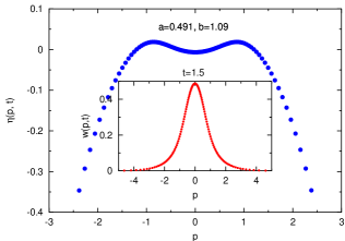
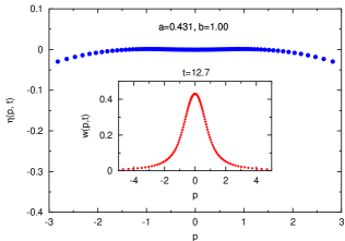
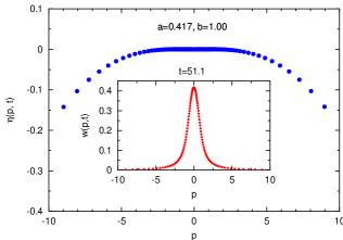
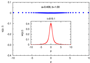
Figure 2: Long time behavior of the quantity $\eta(p,t)$ given in equation (30) and the numerical solutions $w(p,t)$ against an initial probability distribution with triangle shape. The microscopic parameters are set to $p_{c}=1,D=1,\alpha=2$, hence $\kappa=1,\beta=2$. The number of calculated points are $101$. The best fitted parameters $a(t)$ and $b(t)$ in (29) are indicated in each plot. Inset figure shows $w(p,t)$ at each time $t$.

5 The relation between $\beta$ and the average energy

The $\kappa$-Gaussian of the steady-state $w_{s}(p)$ is not normalizable for the parameter region of $2\leq|\kappa|$, or equivalently, $\alpha p_{c}^{2}\leq D$. As similarly as in the momentum distributions in an optical lattice, the physical meaning of this is that compared with the random momentum fluctuations $D$, the capture force $\alpha p_{c}^{2}$ is too weak to keep the particle around the bottom ($p=0$) of the potential $V(p)$. In other words, the potential is too shallow to capture a particle with the large random momentum fluctuations.

Next let us turn our focus on the parameter region of $2/3<|\kappa|<2(D<\alpha p_{c}^{2}<3D)$, in which the second moment

$$\left\langle p^{2}\right\rangle\equiv\int_{-\infty}^{\infty}dp\,p^{2}\,w_{s}(p),$$ (31)

of the $\kappa$-Gaussian becomes infinite. Consequently the mean kinetic energy, $\left\langle p^{2}\right\rangle/2m$, diverges, and it is the hallmark of an anomalous diffusion. Lutz Lutz showed that an explicit correspondence between ergodicity breaking in a system described by power-law tail distributions and the divergences of the moments of these distributions, i.e., Ensemble average and time average of the dynamical variable $p^{n}$ are not equal to each other in the infinite-time limit, when the $2n$-th moment of the stationary momentum distribution for a system described by power-law tail distributions diverges. His analysis is also valid for the present study because both momentum dependent drift coefficient $K^{\rm ol}(p)$ and $K(p)$ have the same asymptotic behavior $\sim-1/p$, and consequently both steady-states are non-Gaussian distributions with power-law tails.

Whereas the mean kinetic energy diverges in this way, in the same region, let us consider the following average energy

$$\left\langle p\frac{d}{dp}V(p)\right\rangle \equiv\int_{-\infty}^{\infty}\frac{p^{2}}{\sqrt{1+\left(\frac{p}{p_{c}}\right)^{4}}}\,w_{s}(p).$$ (32)

Since

$$-\frac{1}{\beta}\frac{d}{dp}\,\exp_{\kappa}\left(-\beta\frac{p^{2}}{2}\right)=\frac{p\exp_{\kappa}\left(-\beta\frac{p^{2}}{2}\right)}{\sqrt{1+\left(\frac{p}{p_{c}}\right)^{4}}},$$ (33)

integrating by part, the r.h.s. of equation (32) becomes

$$-\frac{p}{\beta}\exp_{\kappa}\left(-\beta\frac{p^{2}}{2}\right)\Big{|}_{-\infty}^{\infty}+\frac{1}{\beta}\int_{-\infty}^{\infty}dp\,w_{s}(p)$$ (34)

In the region $2/3<|\kappa|<2$, the first term become zero and the $w_{s}(p)$ is normalizable, thus we finally obtain

$$\left\langle p\frac{d}{dp}V(p)\right\rangle=\frac{1}{\beta}.$$ (35)

This relation remind us a general equipartition principle Tolman ,

$$\left\langle p\frac{\partial}{\partial p}E\right\rangle=k_{\rm B}T,$$ (36)

where $E$ is the energy of a system in thermal equilibrium with the temperature $T$. However, as pointed out before, $\beta$ is not an inverse temperature since the steady-state $w_{s}(p)$ is, in general, a non-equilibrium state, in which the temperature is not well defined.

6 Summary

We have proposed a momentum-dependent drift coefficient which asymptotically decreases as $-1/p$ for a large momentum $|p|>p_{c}$. We have studied a system described by the FP equation with this drift coefficient, and found that the steady-state is a $\kappa$-generalized probability distribution. We performed the several numerical simulations in order to study asymptotic behaviors of the numerical solutions against the different initial probability distributions, and found that these numerical solutions asymptotically approach to the $\kappa$-Gaussian functions.

References

-
(1)
C. Tsallis, J. Stat. Phys. 52, 479-487, (1998)
See, for example, URL http://tsallis.cat.cbpf.br/bibrio.htm - (2) G. Kaniadakis, Physica A 296, (2001) 405-425; G. Kaniadakis and A.M. Scarfone, Physica A 305, 69 (2002); G. Kaniadakis, Phys. Rev. E 66, 056125-1-17, (2002); Phys. Rev. E 72, 036108-1-14, (2005).
- (3) F. Clementi, et. al., Physica A 387, 3201-3208, (2008).
- (4) T. Wada, A.M. Scarfone, AIP Conf. Proc. 965, 177-180, (2007).
- (5) T. Wada, A.M. Scarfone, “Asymptotic solutions of a nonlinear diffusive equation in the framework of -generalized statistical mechanics”, EPJB (2009) to be published.
- (6) T. Wada and H. Suyari, Phys. Lett. A 348, 89, (2006).
- (7) E. Lutz, Phys. Rev. A 67, 051402-1-4, (2003); Phys. Rev. Lett. 93, 190602-1-4, (2004).
- (8) G. Gaeta, Phys. Rev. A 72, 033419 (2005)
- (9) P. Douglas, S. Bergamini, and F. Renzoni, Phys. Rev. Lett. 96, 110601, (2006).
- (10) T.D. Frank, Nonlinear Fokker-Planck Equations, (Springer-Verlag Berlin Heidelberg 2005)
- (11) A.M. Scarfone and T. Wada, Prog. Theor. Phys. Suppl. 162, 45-52 (2006)
- (12) L. Gosse, G. Toscani, SIAM Journal on Numerical Analysis, 43 (2006) 2590 - 2606.
- (13) R.C. Tolman, The Principles of Statistical Mechanics, (Dover Publications, New York, 1938) pp. 93-98