Observations of The Magnetic Reconnection Signature of An M2 Flare on 2000 March 23

Abstract

Multi-wavelength observations of an M 2.0 flare event on 2000 March 23 in NOAA active region 8910 provide us a good chance to study the detailed structure and dynamics of the magnetic reconnection region. In the process of the flare, extreme ultraviolet (EUV) loops displayed two times of sideward motions upon a loop-top hard X-ray source with average velocities of 75 and 25.6 km $s^{-1}$, respectively. Meanwhile part of the loops disappeared and new post-flare loops formed. We consider these two motions to be the observational evidence of reconnection inflow, and find an X-shaped structure upon the post-flare loops during the period of the second motion. Two separations of the flare ribbons are associated with these two sideward motions, with average velocities of 3.3 and 1.3 km $s^{-1}$, separately. The sideward motions of the EUV loops and the separations of the flare ribbons are temporally consistent with two peaks of the X-ray flux. This indicates that there are two times of magnetic reconnection in the process of the flare. Using the observation of photospheric magnetic field, the velocities of the sideward motions and the separations, we deduce the corresponding coronal magnetic field strength to be about 13.2-15.2 G, and estimate the reconnection rates to be 0.05 and 0.02 for these two magnetic reconnection process, respectively. Besides the sideward motions of EUV loops and the separations of flare ribbons, we also observe motions of bright points upward and downward along the EUV loops with velocities ranging from 45.4 to 556.7 km $s^{-1}$, which are thought to be the plasmoids accelerated in the current sheet and ejected upward and downward when magnetic reconnection occurs and energy releases. A cloud of bright material flowing outward from the loop-top hard X-ray source with an average velocity of 51 km $s^{-1}$ in the process of the flare may be accelerated by the tension force of the newly reconnected magnetic field lines. All the observations can be explained by schematic diagrams of magnetic reconnection.

1 Introduction

Solar flares are one of the most spectacular phenomena in solar physics. They are sudden brightening in the solar atmosphere, and consist of a number of components including post-flare loops (Forbes & Priest, 1983; Li & Zhang, 2009), ribbons (Isobe et al., 2002; Ding et al., 2003; Isobe et al., 2005; Temmer et al., 2007), arches (Martin & Svestka, 1988; Tripathi et al., 2006), remote patches (Tang & Moore, 1982; Wang, 2005), surges (Roy, 1973; Jiang et al., 2007), erupting filaments (Gopalswamy & Kundu, 1989; Zhang et al., 2001; Jiang et al., 2006), and other expanding coronal features (Martin, 1989; Wang & Shi, 1992; Zhang & Wang, 2001; Zhang et al., 2007). They have been studied morphologically from direct images (e.g. Krucker & Benz, 2000; Fletcher et al., 2001; Ji et al., 2006) and spectroscopically from spectrograms (e.g. Moore, 1976; Cowan & Widing, 1973; Grigis & Benz, 2005) at different wavelength regions. The theories for solar flares have also been reviewed by many people, such as Parker (1963), Sweet (1969), van Hoven (1976), Priest (1976), Forbes (2003), and Grigis & Benz (2006).

Solar flares are now thought to be caused by magnetic reconnection-the reorganization caused by local diffusion of anti-parallel magnetic field lines in a certain local point in the corona. The tension force of the reconnected magnetic field lines then accelerates the plasma out of the dissipation point. Because of this outflow, the ambient plasma is drawn in. The inflowing plasma carries the surrounding magnetic field lines into the dissipating point. These magnetic field lines continue the reconnection cycle. Therefore, the magnetic energy stored near the dissipation point is released to become the thermal and bulk-flow energy of plasma (Yokoyama et al., 2001). The evidence of magnetic reconnection found by space observations includes the cusp-shaped post-flare loops (Tsuneta et al., 1992), the loop-top hard X-ray source (Masuda et al., 1994), the reconnection inflow (Yokoyama et al., 2001; Lin et al., 2005; Narukage & Shibata, 2006), downflows above post-flare loops (McKenzie & Hudson, 1999; Innes et al., 2003; Asai et al., 2004), plasmoid ejections (Shibata et al., 1995; Ohyama & Shibata, 1997; Ohyama & Shitaba, 1998), etc. The magnetic reconnection model proposed by Carmichael (1964), Sturrock (1966), Hirayama (1974), and Kopp & Pneuman (1976) (the CSHKP model) suggests that magnetic field lines successively reconnect in the corona. This model explains several well-known features of solar flares, such as the growth of flare loops with a cusp-shaped structure and the formation of the H$\alpha$ two-ribbon structures at their footpoints. In recent decades, this model has been further extended (e.g. Moore et al., 2001; Yokoyama & Shibata, 2001; Priest & Forbes, 2002; Lin, 2004)

In this paper, we analysis a flare event to investigate the detailed structure and dynamics of the reconnection region. We show the observational data in section 2, and the corresponding results in section 3. Conclusions and brief discussion are presented in section 4.

2 Observations

On 2000 March 23, an M 2.0 flare occurred near the solar limb (N15 W69) in NOAA active region (AR) 8910. This flare started at 11:32 UT and ended at 12:30 UT, with a peak at 12:14 UT. It was observed by several satellites including: Transition Region and Coronal Explorer (TRACE; Handy et al., 1999), Solar and Heliospheric Observatory (SOHO), YOHKOH and GOES. In this paper, we use TRACE 195 Å images, with 10 s temporal resolution and 1″ spatial resolution, to study the dynamics of the extreme ultraviolet (EUV) loops during the flare, and 1600 Å data, with 1″ spatial resolution and 1 minute temporal resolution, to research the kinetics of the flare ribbons. The evolution of the magnetic fields and the sunspots in the source region of the flare is studied using SOHO/Michelson Doppler Imager (MDI; Scherrer et al., 1995) magnetograms and TRACE WL images. We also employ observations of YOHKOH/Hard X-ray Telescope (HXT; Kosugi et al., 1991) and GOES to explore the X-ray variation of the event.

3 Results

The general information of this event is exhibited in Fig. 1. Figure 1a shows the longitudinal magnetogram of the source AR of the flare observed by SOHO/MDI, and indicates that this AR has a mixture of polarities and further complicated magnetic neutral lines. In order to make sure the polarities of the magnetic fields without the limb effect, we investigate all the observations of SOHO/MDI from 2000 March 20, when the AR was in the center of the solar disk, to 2000 March 23, when the flare occurred, and find that all the polarities of the magnetic fields associated with the flare are true, denoted by P1, P2, P3 and P4 for positive ones, while N1, for negative. The continuum intensity observed by TRACE WL is displayed in Fig. 1b. Figure 1c exhibits TRACE 1600 Å image. This flare is a complicated one with several flare ribbons shown as FR1, FR2 and FR3. We overlay the magnetic fields shown in Fig. 1a as white and black contours on Fig. 1c, and find that the southern flare ribbon FR1, a simple one, foots around N1, while the northern flare ribbons FR2 and FR3, more complicated, around P2, P3 and P4. Figures 1d-1f show the time sequence of TRACE 195 Å images. Before the occurrence of the flare, there were a set of EUV loops in the AR marked as L1 in Fig. 1d. Comparing Fig. 1d with Figs. 1a-1c, we notice that L1 connects P1 and N1.

3.1 Loop dynamics

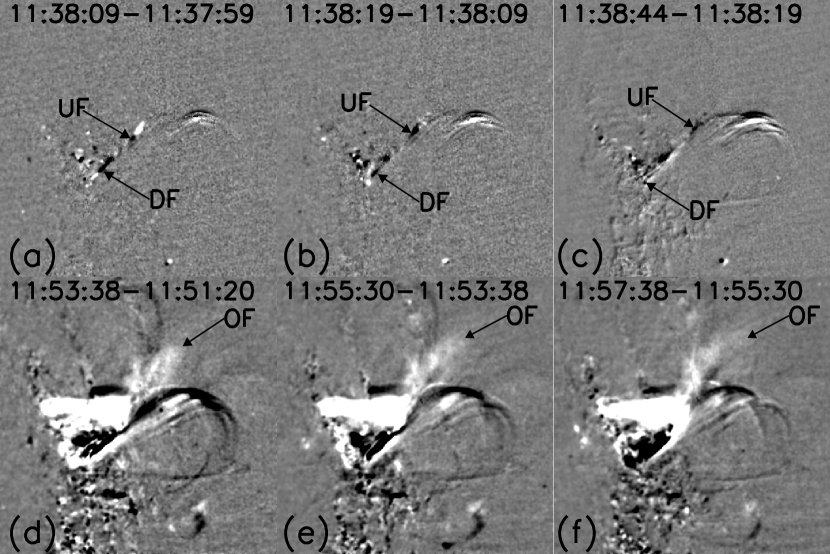
Figure 4: Time sequence of running difference images observed by TRACE 195 Å showing the motions of plasmoids upward flow (UF) and downward flow (DF) along loops (a-c), and outflow (OF) of plasmoids (d-f). The FOV is 175″$\times$ 175″.

From about 11:35 UT, a sideward motion of L1 appeared from southwest to northeast, i.e. along the solid line BA shown in Fig. 1d, meanwhile L1 partly disappeared. After several minutes of this motion, new post-flare loops denoted by PFLs1 in Fig. 1e appeared. Comparing Fig. 1e with Fig. 1c, we find that the southern leg of PFLs1 foots at FR1, while the northern one, at FR2. The contours on Fig. 1d represent the hard X-ray emissions in the L energy band (14-23 keV) observed by Yohkoh/HXT at 11:35 UT (see the left vertical arrow in Fig. 4d). The majority of the hard X-ray sources, which can be considered as footpoint sources, are co-spatial with the flare ribbons, and a source marked as LTS1, which also appears in the M1 energy band (23-33 keV) image, a loop-top one. The height of LTS1 to footpoint sources (see the two-head arrows in Fig. 1d) is about 20 Mm. As this flare is a limb event, the projection effect must be considered. We assume that the line along the two-head arrows is vertical to the local photosphere, and its heliographic position is the same to the AR (N15 W69). Then the height $H_{corrected}$ after correction

$$H_{corrected}=\frac{H_{measured}}{\sqrt{(\sin 15)^{2}+(\cos 15)^{2}(\sin 69)^{2}}}$$ (1)

is 22.7 Mm, where $H_{measured}$ is the measured value. The physical parameters mentioned below, e.g. the length of the current sheet, which are similar to the height of LTS1, are corrected using the same method. The loops marked as L11 in Fig. 1e, which was part of L1, moved toward the northeast from 11:43 UT, and disappeared at 11:44 UT.

From about 11:49 UT, another sideward motion of L1 was detected at a higher position from southeast to northwest, i.e. along the solid line DC (shown in Fig. 1f), and another set of post-flare loops marked as PFLs2 in Fig. 1f appeared. Comparing Fig. 1f with Fig. 1c, we note that the southern leg of PFLs2 also foots at FR1, but the northern one, at FR3. By overlaying the contour of a hard X-ray image observed by Yohkoh/HXT at 12:06 UT (see the right vertical arrow in Fig. 4d) on Fig. 1f, we find that there is also a loop-top source marked as LTS2, with a height of 30 Mm (34 Mm after correction). From Figs. 1d-1f, we uncover that L1 firstly undergoes sideward motion and partly disappears, then post-flare loops form. Furthermore, the hard X-ray sources (LTS1 and LTS2) locate upon the top of post-flare loops, and under the region where the loops show maximum sideward motion velocities.

The second sideward motion of L1 lasts for a longer time (22 minutes) than the first one (6 minutes), and the flare is more powerful in this period, so we study it in detail. Figure 2 displays the time sequence of TRACE 195 Å images showing the second sideward motion. The dotted lines in Figs. 2a-2b represent the EUV loops at 11:54:24 UT. From these two figures, we can see clearly the sideward motion (denoted by a white arrow in Fig. 2b). When two approaching loops met, the motion of these loops stopped, but there were still some neighboring loops moved toward the meeting region continuously. The distance between these two EUV loops is almost constant with a value of 0.3-0.7 Mm (shown by two black arrows in Fig. 2c). We assume that the direction of the sideward motions is perpendicular to the line of sight, so the projection effect to the distance can be neglected. The physical parameters mentioned below, e.g. the velocities of sideward motions, which are similar to the distance, are not necessary to be corrected for the projection effect. The dashed lines in Fig. 2c, the outer edges of the EUV loops, show an X-shaped structure. From 11:58:11 UT, the second set of post-flare loops (denoted as PFLs2 in Fig. 2d) appeared with a cusp-shaped structure (see CUSP in Fig. 2d) riding on it. Before 11:59 UT, the shape of L1 was smooth, then an abrupt break occurred accompanying with the appearance of a brightening point “B” (see Fig. 2d). After the break, several other bright points, such as “BP” marked in Fig. 2e, appeared above the “B” point, and propagated upward along L1 (see the white solid arrow in Fig. 2e). The EUV loops L (arrowed in Fig. 2d) under the “B” point disappeared after several minutes of the break, only the post-flare loops PFLs2 and the cusp-shaped structure CUSP left (see Fig. 2f). We estimate the length of the loops between “B” point and CUSP to be 12-15 Mm (shown by the two-head solid arrows in Fig. 2d), that is 13.6-17 Mm after correction.

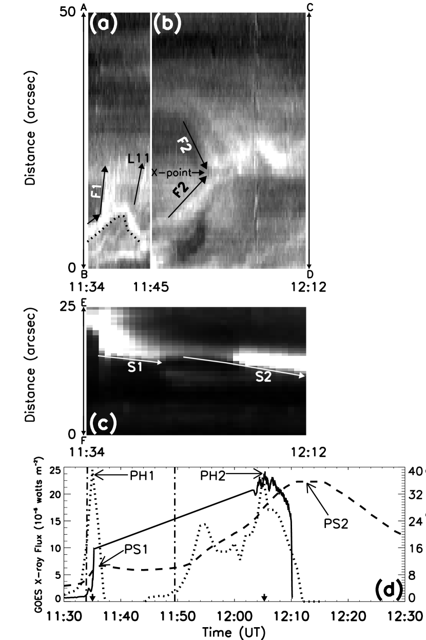
Figure 3: (a)-(c): Time evolution of the one-dimension distribution of TRACE 195 Å and 1600 Å intensity along the solid lines AB, CD, EF specified in Fig. 1, respectively. F1 and F2 represent the sideward motions of the EUV loops, as well as S1 and S2, the separations of FR1. The dotted line in (a) outlines the out edges of loops. (d): The time integrated hard X-ray flux (solid curves) from YOHKOH/HXT, the GOES-10 1-8 Å soft X-ray flux (dashed curves) and their time derivative (dotted curves). PS1-PS2 and PH1-PH2 represent the peaks of these flux. The vertical dash-dotted lines represent the beginning times of the sideward motions, and the two vertical solid arrows, the times when we obtained hard X-ray images (see the contours in Figs. 1d and 1f).

In order to quantificationally study the sideward motions of the EUV loops, we make a time slice along the moving directions of L1, and show them in Figs. 3a and 3b. Figure 3a presents the time evolution of the one-dimension distribution of EUV intensity of the loops along BA from 11:34 to 11:45 UT. In this figure, the left arrows marked as F1 show the first sideward motion with an average velocity of 75 km $s^{-1}$. The dotted line indicates that part of L1 first moved along BA, then returned after several minutes. Furthermore, a small portion of the returning loops also displayed a sideward motion along BA, as denoted by L11 (see also Fig. 1e), with an average velocity of 70 km $s^{-1}$. Figure 3b is the time slice of the second main sideward motion of L1 along DC from 11:45 to 12:12 UT. A clear merging pattern (see also in Fig. 2) arrowed as F2 can be seen with an average velocity of 25.6 km $s^{-1}$.

3.2 Flare ribbon kinetics and X-ray flux properties

In the CSHKP model, the reconnection points move upward, therefore, newly reconnected field lines have their footpoints further out than that of the field lines which have already reconnected, which leads us to recognize the “apparent” separation motion of the flare ribbons (Asai et al., 2004). We exhibit the time evolution of the one-dimensional distribution of 1600 Å intensity of FR1 along the solid line FE (see Fig. 1c) from 11:34 to 12:12 UT in Fig. 3c. There are two clear separations shown as S1 and S2 with the average velocities of 3.3 and 1.3 km $s^{-1}$, respectively. Between these two separations, FR1 became too weak to be observed.

Figure 3d shows GOES-10 1-8 Å soft X-ray flux (dashed curve) of this flare, and indicates that there are two peaks (PS1 and PS2) of the flux at 11:37 and 12:14 UT, separately. The solid curve shows the time integrated hard X-ray flux observed by YOHKOH/HXT. Unfortunately, there are no observations between 11:36 and 12:03 UT. As there is a good correlation between the time derivative of soft X-ray flux and the hard X-ray one (Dennis & Zarro, 1993), we use the time derivative (the dotted curves) of GOES soft X-ray flux to extrapolate the change of the hard X-ray one during the observational gap. Comparing the hard X-ray flux (solid curves) with the time derivative (dotted curves), we find that the peaks of these two flux curves are similar. There are two peaks (PH1 and PH2) which correspond with PS1 and PS2. The vertical dash-dotted lines represent the beginning time of two sideward motions. From Fig. 3, we notice that the two sideward motions (F1 and F2) of L1, the two separations (S1 and S2) of FR1, and the two peaks (PS1 and PS2, PH1 and PH2) of X-ray flux are temporally consistent.

3.3 Plasma ejections

Besides the sideward motions of the EUV loops and the separations of the flare ribbons, we also find plasma ejections in the process of the flare. Immediately after the beginning of the sideward motion, lots of bright points appeared and propagated upward and downward along the loops. We show an example of a pair of bright points in Figs. 4a-4c. These figures display the running difference images of TRACE 195 Å from 11:37:59 to 11:38:44 UT. From these images, we find a black point (arrowed by UF) moving upward along L1, with an average velocity of 221.2 km $s^{-1}$ (251.3 km $s^{-1}$ after correction), as well as another black point (denoted by DF), downward, with an average velocity of 167.3 km $s^{-1}$, which is 190.1 km $s^{-1}$ after correction. The upward and downward motions of bright points existed all the time during the flare. During the process of the first sideward motion, the upward bright points appeared always higher than the region where the loops displayed maximum motion velocities, and the downward ones, under that region. Both of them propagated along L1. In the process of the second sideward motion, the upward bright points appeared upon the bright point “B” and moved along the right leg of the X-shaped structure, while the downward ones, appeared under the cusp-shaped structure and moved along the right leg of PFLs2. The area of the moving bright points ranges from 1.5 to 23 $Mm^{2}$, with an average value of 9.1 $Mm^{2}$. The moving speeds of the bright points range from 40 to 490 km $s^{-1}$ (45.4-556.7 km $s^{-1}$ after correction), with an average value of 172 km $s^{-1}$ (195.4 km $s^{-1}$ after correction).

Moreover, we find an outflow of a bright cloud. Figures 4d-4f show a series of TRACE 195 Å running difference images. The cloud of the bright material (arrowed by OF) went away upon the loop-top hard X-ray source LTS2 with velocities of 25.4-79.4 km $s^{-1}$ (28.9-90.2 km $s^{-1}$ after correction) and an average value of 44.9 km $s^{-1}$ (51 km $s^{-1}$ after correction). In the propagating process of the outflow, these bright material became diffused, and disappeared after 20 minutes.

4 CONCLUSIONS AND DISCUSSION

In this paper, we analyze an M 2.0 flare on 2000 March 23 at N15 W69 for detail, and get the following results: 1. Long EUV loops undergo two times of sideward motions and partly disappear, subsequently two sets of post-flare loops form. 2. There are two peaks in the X-ray flux of the flare. Each peak is temporally consistent with a phase of the sideward motion of the EUV loops and the separation of the flare ribbons. 3. Bright points eject along the EUV loops upward and downward all the time during the flare. 4. An outflow of a bright cloud moves away from the loop-top hard X-ray source region.

It is well accepted that magnetic reconnection in solar corona results in solar flares. Masuda et al. (1994) suggested that magnetic reconnection takes place around or above the loop-top hard X-ray source. In our study, the sideward motions and disappearances of EUV loops also take place above the loop-top hard X-ray sources (see Figs. 1d and 1f), which may be consistent with that of Masuda et al.. Tsuneta et al. (1992) observed cusp-shaped post-flare loops, and suggested that an X-type or Y-type reconnection point wound be formed at the top of the cusp. In the process of the second sideward motion, we find an X-shaped structure above the cusp-shaped post-flare loops (see Fig. 2) which is identical with the X-type current sheet mentioned by Tsuneta et al., and the sideward motions can be considered as reconnection inflows. As the two peaks of the X-ray flux are relevant to the two times of sideward motions of loops and separations of flare ribbons, we consider that there are two magnetic reconnection process in this flare.

Although much evidence has been found to support the magnetic reconnection mechanism, the slow and fast shocks predicted by reconnection theories (Petschek, 1964; Forbes & Priest, 1983; Ugai, 1987) have not yet been identified. For the detailed observations of the flare, we have the chance to search for the signature of shocks associated with magnetic reconnection. Shiota et al. (2003) once performed MHD simulations of a giant arcade formation with a model of magnetic reconnection coupled with heat conduction, and showed that the Y-shaped structure was identified to correspond to the slow and fast shocks associated with the magnetic reconnection. In this work, we study the physical parameters at the similar positions and similar times of the simulation of Shiota et al.. Figure 5a shows the distributions of several physical quantities, e.g. temperature, emission measure and brightness, along the white line GH (see Fig. 2c) at 11:58:11 UT. The temperature and emission measure are calculated from a wavelength pair (171 and 195 Å) of two TRACE images. From Fig. 5a, we can see a discontinuous region “I” between two dash-dotted lines which is similar to the simulated slow shock. It may be the observational evidence of the slow shock associated with magnetic reconnection. Masuda et al. (1994) once suggested that the hard X-ray source above the loop top in an impulsive flare may be a fast shock created by the collision of a reconnection jet with the flare loop. The hard X-ray source LTS2 above the top of post-flare loops and the slightly brighter cross points of the X-shaped structure may be the observational evidence of fast shocks. In order to confirm this, we show the distributions of some physical quantities along the white line IJ (see Fig. 2c) in Fig. 5b. There are two discontinuous regions (“II” and “III”) between the dash-dotted lines. The difference between these two regions may be caused by the different local magnetic field configurations. By comparing our observations with the simulations of Shiota et al., we find that these two discontinuous regions may be identical with the fast shocks. Therefore, the X-shaped structure may correspond to the slow and fast MHD shocks associated with magnetic reconnection.

A similar process of reconnection inflow was reported by Yokoyama et al. (2001) for the event on 1999 March 18 with an inflow velocity of 1.0-4.7 km $s^{-1}$. Lin et al. (2005) showed another example of reconnection inflow by analyzing a flare event on 2003 November 18, and gave out the average velocities of 10.5-106 km $s^{-1}$. Narukage & Shibata (2006) statistically analyzed six reconnection inflows in solar flares observed with SOHO/EIT, and found the inflow velocities were about 2.6-38 km $s^{-1}$. We use TRACE data with higher spatial and temporal resolutions to get the inflow velocities to be 75 and 25.6 km $s^{-1}$, more likely consistent with Lin et al.. In the process of the flare, we also observe two times of separations of flare ribbon. Using the conservation of magnetic flux

$$v_{inflow}B_{corona}=v_{foot}B_{photo},$$ (2)

we can estimate the coronal magnetic field strength $B_{corona}$, where $B_{photo}$ and $v_{foot}$ are the photospheric magnetic field strength and separation velocity of the flare ribbons (Isobe et al., 2002). From this equation, we get $B_{corona}$ as

$$B_{corona}=B_{photo}\frac{v_{foot}}{v_{inflow}}.$$ (3)

For the two times of magnetic reconnection, the ratios of the separation velocities of flare ribbons to inflow velocities of EUV loops are 0.044 and 0.051 respectively, one order of magnitude smaller than that of Narukage & Shibata (2006). The average magnetic field strength in the photosphere of this AR is about 300 G. Then $B_{corona}$ is about 13.2 and 15.2 G during the process of the two times of magnetic reconnection, respectively. The local Alfvén velocity $v_{A}$ is expected as

$$v_{A}=\frac{B_{corona}}{\sqrt{4\pi\rho}}=\frac{B_{corona}}{\sqrt{4\pi m_{p}n_{p}}},$$ (4)

where $m_{p}$=1.67$\times$10^-24 g is the proton mass and $n_{p}$ is the proton number density outside the current sheet which is 4$\times$10⁸ $cm^{-3}$ (Yamamoto et al., 2002; Isobe et al., 2002). We use 14 G as $B_{corona}$ to calculate $v_{A}$ and obtain it to be 1530 km $s^{-1}$, then estimate the reconnection rate $M_{A}$

$$M_{A}=\frac{v_{inflow}}{v_{A}}$$ (5)

to be 0.05 and 0.02 in two process of magnetic reconnection, separately. They are bigger than Yokoyama et al. (0.001-0.03) and Narukage & Shibata (0.001-0.07), and smaller than Lin et al. (0.01-0.23). During the second sideward motion, we obtain the distance between the X-shaped EUV loops to be 0.3-0.7 Mm. If the distance is the width of the current sheet in this flare, it should be the upper limit, and is two orders of magnitude smaller than that of Lin et al. (2007). We estimate the length of the current sheet to be the distance between the top of the cusp-shaped structure and the “B” point (see the two-head solid arrows in Fig. 2c), and get a value of 13.6-17 Mm. According to Sweet-Parker model, if the plasma compressibility is neglected, the reconnection rate is given by the ratio of width to length of the current sheet (Priest & Forbes, 2002). So we calculate the reconnection rate to be 0.02-0.05 which is similar with those values (0.05 and 0.02) we estimated above. The height of the loop-top hard X-ray source of two magnetic reconnections are 22.7 and 34 Mm which may represent the height of the lower parts of the current sheet. Both of these heights are much lower than that of Yokoyama et al. (2001), Lin et al. (2005) and Narukage & Shibata (2006).

In the process of magnetic reconnection, many bright points ejected along the EUV loops upward and downward. These ejections may be plasmoids accelerated in current sheet. McKenzie & Hudson (1999) examined the super-arcade downflow motions sunward from the high corona with speeds of 45-500 km $s^{-1}$. Innes et al. (2003) found that highly blueshift features, which correspond to a Doppler velocity of up to 1000 km $s^{-1}$, were associated with the downflows using SUMER and TRACE observations. Asai et al. (2004) found downflows with velocities from 30 to 500 km $s^{-1}$. They also illustrated that the times when the downflow motions started to be seen corresponded to the times when bursts of non-thermal emissions in hard X-rays and microwaves were emitted. Lin et al. (2005) pointed out an average outflow velocity ranged from 640 to 1075 km $s^{-1}$. The velocities of the upflows and downflows in our paper are 45.4-556.7 km $s^{-1}$, consistent with the results mentioned above. In section 3.3, we described an outflow of a bright cloud from the reconnection site. The bright cloud is plasmoids which may be accelerated by the tension force of newly reconnected magnetic field lines.

All the observations of the magnetic reconnection signature of the flare can be explained by schematic diagrams shown in Fig. 6. In order to better compare these diagrams with the observations, we use the same expressions of physical parameters mentioned in section 3. The dashed lines L2 and L3 are deduced from the information of magnetic field structures, flare ribbon evolutions and post-flare loop dynamics. Before the flare, there are three main loops in this AR marked as L1, L2 and L3 in Fig. 6a. Because of some disturbance, two anti-parallel field lines L1 and L2 meet resulting in the formation of a current sheet. Then part of L1 and L2 are broken and reconnect, the flare begins. As a result of this reconnection, the inflow F1 (shown by the thick solid arrow in Fig. 6a), the newly formed post-flare loops PFLs1 (arrowed in Fig. 6b), and the upward and downward propagating plasmoids DF and UF (displayed by the hollow thick arrows in Fig. 6b) appear. Several minutes later, another reconnection occurs between L1 and L3. As a result of this reconnection, the inflow F2 (displayed by the thick solid arrows in Fig. 6b), the newly formed post-flare loops PFLs2 (arrowed in Fig. 6c), and downflows and upflows of accelerated plasmoids DF and UF (shown by the hollow thick arrows in Fig. 6c) take place. The outer edges of L1 and L3 form a cusp-shaped structure CUSP (arrowed in Fig. 6c) and an X-shaped structure. The tension force of the reconnected magnetic field lines accelerates the plasmoids out of the current sheet, then the outflow OF (marked by the thick solid in Fig. 6c) appears.

Figure 1: (a): A longitudinal magnetogram observed by SOHO/MDI. P1-P4 represent the positive magnetic fields; and N1, the negative magnetic field. (b-c): TRACE WL and 1600 Å  images. FR1-FR3 are the flare ribbons. (d-f): TRACE 195 Å images showing the evolution of EUV loops. PFLs1 and PFLs2 denote the post-flare loops, L1 and L11, the EUV loops, LTS1 and LTS2, the loop-top hard X-ray sources. The white window in (f) represents the field of view (FOV) in Fig. 2. The solid lines AB, CD, EF in (c), (d) and (f) show the position for time slice evolution shown in Fig. 3. The contours in (c) show the magnetic fields of the active region, while in (d) and (f), the hard X-ray emission observed by YOHKOH/HXT. The dotted lines in (d) and (f) connect two footpoint hard X-ray sources, and the two-head arrows represent the distance from the dotted lines to the loop-top sources. The FOV is 200″$\times$ 200″.

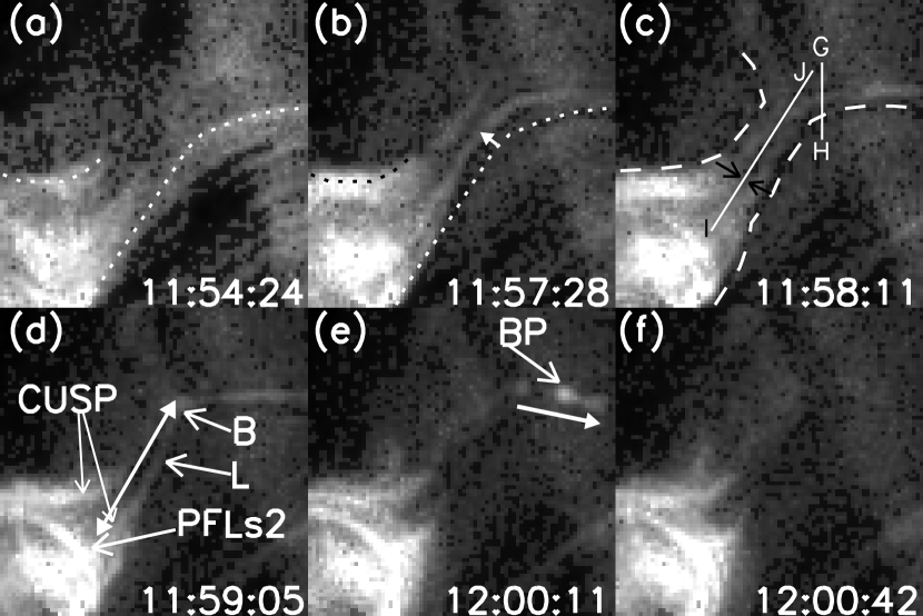
Figure 2: Time sequence of TRACE 195 Å images showing the evolution of the loops. The dotted lines in (a) and (b) represent the loops at 11:54:24 UT, as well as the dashed lines in (c), the out edges of loops at 11:58:11 UT. The solid arrow in (b) represents the moving direction of the loops, as well as the solid arrow in (e), the moving direction of the bright point. The two black arrows in (c) display the distances between two EUV loops, and the solid two-head arrows in (d), the length of EUV loops. CUSP means the cusp-shaped structure, PFLs2, the post-flare loops, L, EUV loop, B, break point, BP, bright point. The white solid lines GH and IJ in (c) show the position for the distributions of several physical quantities displayed in Fig. 5. The FOV is 40″$\times$ 40″.

Figure 5: The distributions of brightness (solid curves), temperature (dotted curves) and emission measure (dashed curves) along the white solid lines GH (a) and IJ (b) shown in Fig. 2c. The dash-dotted lines in (a) and (b) outline the discontinuous regions “I”, “II” and “III”.

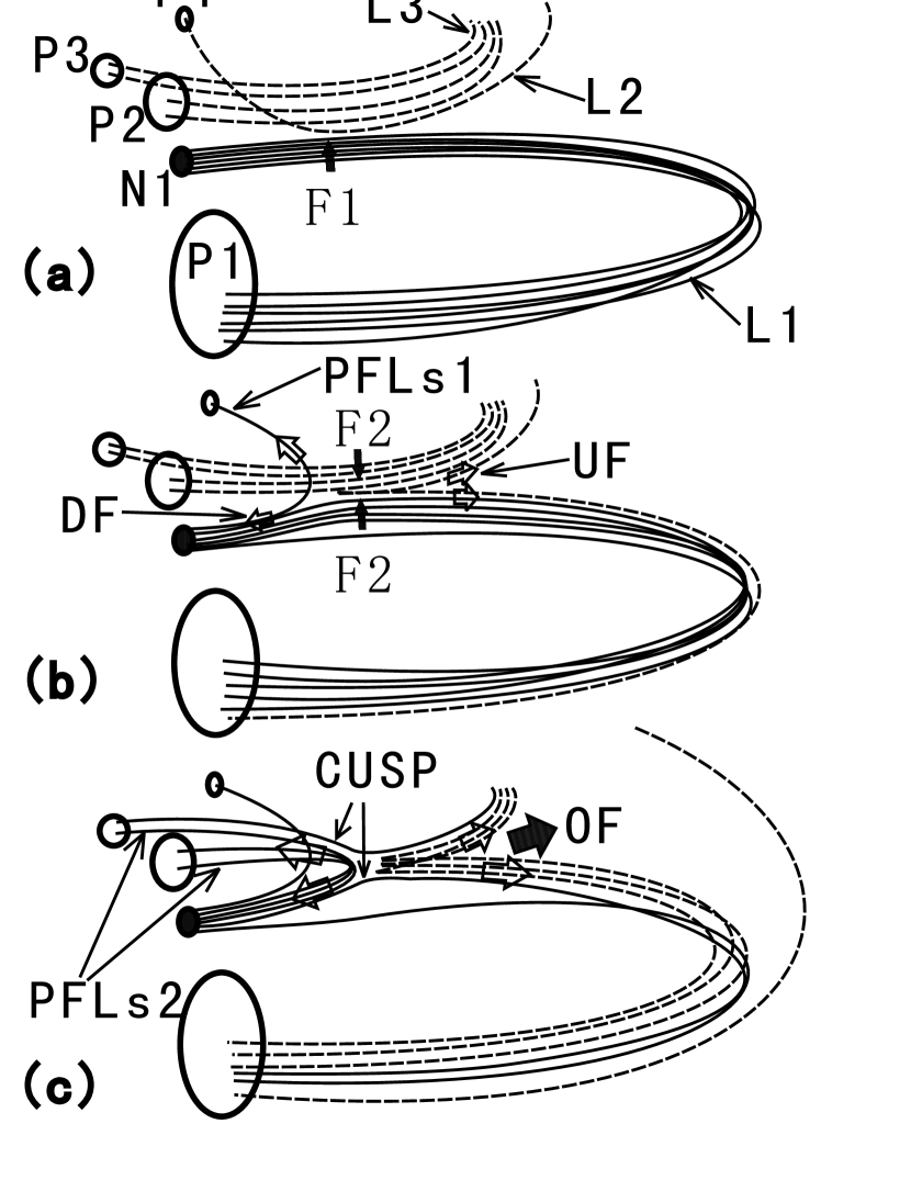
Figure 6: The schematic diagrams illustrating the evolution of the flare event on 2000, March 23. The ellipses represent the sunspots in the active region. The lines (L1-L3) show the loops, and PFLs1 and PFLs2, the post-flare loops. CUSP shows the cusp-shaped structure. The solid thick arrows in (a) and (b) display the directions of the sideward motions, as well as the hollow thick arrows in (b) and (c), upflow (UF) and downflow (DF) of plasmoids. The solid arrow in (c) shows the outflow (OF) of plasmoids.

References

- Asai et al. (2004) Asai, A., Yokoyama, T., Shimojo, M., & Shibata, K. 2004, ApJ, 605, L77
- Carmichael (1964) Carmichael, H. 1964, in The Physics of Solar Physics, ed. W. N. Hess (NASA SP-50; Washington, DC: NASA), 451
- Cowan & Widing (1973) Cowan, R. D., & Widing, K. G. 1973, ApJ, 180, 285
- Dennis & Zarro (1993) Dennis, B. R., & Zarro, D. M. 1993, Sol. Phys., 146, 177
- Ding et al. (2003) Ding, M. D., Chen, Q. R., Li, J. P., & Chen, P. F. 2003, ApJ, 398, 683
- Fletcher et al. (2001) Fletcher, L., Metcalf, T. R., Alexander, D., Brown, D. S., & Ryder, L. A., 2001, ApJ, 554, 451
- Forbes & Priest (1983) Forbes, T. G., & Priest, E. R. 1983, Sol. Phys., 88, 211
- Forbes (2003) Forbes, T. G. 2003, Adv. Space Res., 32, 1043
- Gopalswamy & Kundu (1989) Gopalswamy, N., & Kundu, M. R. 1989, Sol. Phys., 122, 91
- Grigis & Benz (2005) Grigis, P. C., & Benz, A. O. 2005, A&A, 434, 1173
- Grigis & Benz (2006) Grigis, P. C., & Benz, A. O. 2006, A&A, 458, 641
- Handy et al. (1999) Handy, B. N., et al. 1999, Sol. Phys., 187, 229
- Hirayama (1974) Hirayama, T. 1974, Sol. Phys., 34, 323
- Innes et al. (2003) Innes, D. E., McKenzie, D. E., & Wang, T. 2003, Sol. Phys., 217, 267
- Isobe et al. (2002) Isobe, H., et al. 2002, ApJ, 566, 528
- Isobe et al. (2005) Isobe, H., Takasaki, H., & Shibata, K. 2005, ApJ, 632, 1184
- Ji et al. (2006) Ji, H. S., et al. 2006, ApJ, 636, 173
- Jiang et al. (2006) Jiang, Y. C., Li, L. P., Yang, L. H. 2006, Chin. J. Astron. Astrophys., 6, 345
- Jiang et al. (2007) Jiang, Y. C., Chen, H. D., Li, K. J., Shen, Y. D., & Yang, L. H. 2007, A&A, 469, 331
- Kopp & Pneuman (1976) Kopp, R. A., & Pneuman, G. W. 1976, Sol. Phys., 50, 85
- Kosugi et al. (1991) Kosugi, T., et al. 1991, Sol. Phys., 136, 17
- Krucker & Benz (2000) Krucker, S., & Benz, A. O. 2000, Sol. Phys., 191, 341
- Li & Zhang (2009) Li, L. P., & Zhang, J. 2009, ApJ, 690, 347
- Lin (2004) Lin, J. 2004, Sol. Phys., 222, 115
- Lin et al. (2005) Lin, J., et al. 2005, ApJ, 622, 1251
- Lin et al. (2007) Lin, J., et al. 2007, ApJ, 658, L123
- Martin & Svestka (1988) Martin, S. F., & Svestka, Z. F. 1988, Sol. Phys., 116, 91
- Martin (1989) Martin, S. F. 1989, Sol. Phys., 121, 215
- Masuda et al. (1994) Masuda, S., Kosugi, T., Hara, H., Tsuneta, S., & Ogawara, Y. 1994, Nature, 371, 495
- McKenzie & Hudson (1999) McKenzie, D. E., & Hudson, H. S. 1999, ApJ, 519, L93
- Moore (1976) Moore, R. L. 1976, BAAS, 8, 549
- Moore et al. (2001) Moore, R. L., Sterling, A. C., Hudson, H. S., & Lemen, J. M. 2001, ApJ, 552, 833
- Narukage & Shibata (2006) Narukage, N., & Shibata, K. 2006, ApJ, 637, 1122
- Ohyama & Shibata (1997) Ohyama, M., & Shibata, K., 1997, PASJ, 49, 249
- Ohyama & Shitaba (1998) Ohyama, M., & Shibata, K., 1998, ApJ, 499, 934
- Parker (1963) Parker, E. N. 1963, ApJS, 8, 177
- Petschek (1964) Petschek, H. E. 1964, in Proc. AAS-NASA Symp. on the Physics of Solar Flares, ed. W. N. Hess (NASA SP-50), 425
- Priest (1976) Priest, E. R. 1976, Sol. Phys., 47, 41
- Priest & Forbes (2002) Priest, E. R., & Forbes, T. G. 2002, A&AR, 10, 313
- Roy (1973) Roy, J. R. 1973, Sol. Phys., 28, 95
- Scherrer et al. (1995) Scherrer, P. H., et al. 1995, Sol. Phys., 162, 129
- Shibata et al. (1995) Shibata, K., Masuda, S., Shimojo, M., Hara, H., Yokoyama, T., Tsuneta, S., Kosugi, T., & Ogawara, Y. 1995, ApJ, 451,L83
- Shiota et al. (2003) Shiota, D., Yamamoto, T. T., Sakajiri, T., Isobe, H., Chen, P. F., & Shibata, K. 2003, PASJ, 55, L35
- Sturrock (1966) Sturrock, P. A. 1966, Nature, 211, 695
- Sweet (1969) Sweet, P. A. 1969, ARA&A, 7, 149
- Tang & Moore (1982) Tang, F., & Moore, R. L. 1982, Sol. Phys., 77, 263
- Temmer et al. (2007) Temmer, M., Veronig, A. M., Vrs̆nak, B., & Miklenic, C. 2007, ApJ, 654, 665
- Tsuneta et al. (1992) Tsuneta, S., et al., 1992, PASJ, 44, L63
- Tripathi et al. (2006) Tripathi, D., Isobe, H., & Mason, H. E. 2006, A&A, 453, 1111
- Ugai (1987) Ugai, M. 1987, Geophys. Res. Lett., 14, 103
- van Hoven (1976) van Hoven, G. 1976, Sol. Phys., 45, 95
- Wang (2005) Wang, H. M. 2005, ApJ, 618, 1012
- Wang & Shi (1992) Wang, J. X., & Shi, Z. X. 1992, Sol. Phys., 140, 67
- Yamamoto et al. (2002) Yamamoto, T. T., Shiota, D., Sakajiri, T., Akiyama, S., Isobe, H., & Shibata, K. 2002, ApJ, 579, L45
- Yokoyama et al. (2001) Yokoyama, T., Akita, K., & Newmark, J. 2001, ApJ, 546, L69
- Yokoyama & Shibata (2001) Yokoyama, T., & Shibata, K. 2001, ApJ, 549, 1160
- Zhang & Wang (2001) Zhang, J., & Wang, J. X. 2001, ApJ, 554, 474
- Zhang et al. (2001) Zhang, J., Wang, J. X., Deng, Y. Y., & Wu, D. J. 2001, ApJ, 548, L99
- Zhang et al. (2007) Zhang, J., Li, L. P., & Song, Q. 2007, ApJ, 662, L35