Magnetoconductance of the quantum spin Hall state

Abstract

We study numerically the edge magnetoconductance of a quantum spin Hall insulator in the presence of quenched nonmagnetic disorder. For a finite magnetic field $B$ and disorder strength $W$ on the order of the bulk gap $E_{g}$, the conductance deviates from its quantized value in a manner which appears to be linear in $|B|$ at small $B$. The observed behavior is in qualitative agreement with the cusp-like features observed in recent magnetotransport measurements on HgTe quantum wells. We propose a dimensional crossover scenario as a function of $W$, in which for weak disorder $W<E_{g}$ the edge liquid is analogous to a disordered spinless 1D quantum wire, while for strong disorder $W>E_{g}$, the disorder causes frequent virtual transitions to the 2D bulk, where the originally 1D edge electrons can undergo 2D diffusive motion and 2D antilocalization.

I Introduction

A great deal of interest has been generated recently by the theoretical predictionBernevig et al. (2006) and experimental observationKönig et al. (2007); Roth et al. (2009); Büttiker (2009) of the quantum spin Hall (QSH) insulator state Kane and Mele (2005); Bernevig and Zhang (2006); König et al. (2008). The QSH state is a novel topological state of quantum matter which does not break time-reversal symmetry (TRS), but has a bulk insulating gap and gapless edge states with a distinct helical liquid property Wu et al. (2006). The gaplessness of the edge states is protected against weak TRS preserving perturbations by Kramers degeneracy Wu et al. (2006); Xu and Moore (2006). As a result, the QSH state exhibits robust dissipationless edge transport König et al. (2007); Roth et al. (2009); Büttiker (2009) in the presence of nonmagnetic disorder.

However, in the presence of an external magnetic field which explicitly breaks TRS, the gaplessness of the edge states is not protected. This can be simply understood by considering the generic form of the effective one-dimensional (1D) Hamiltonian $H$ for the QSH edge Qi et al. (2008) to first order in the magnetic field $\mathbf{B}$, $H=H_{0}+H_{1}(\mathbf{B})$, where $H_{0}=\hbar vk\sigma_{3}$ is the Hamiltonian of the unperturbed edge, and $H_{1}(\mathbf{B})=\sum_{a=1,2,3}(\mathbf{t}_{a}\cdot\mathbf{B})\sigma_{a}$ is the perturbation due to the field. $k$ is a 1D wave vector along the edge, $v$ is the edge state velocity, $\sigma_{1,2,3}$ are the three Pauli spin matrices, and $\mathbf{t}_{1,2,3}$ are model-dependent coefficient vectorsQi et al. (2008). If $\mathbf{B}$ points along a special direction in space $\mathbf{t}^{*}\equiv\mathbf{t}_{1}\times\mathbf{t}_{2}$, then $H_{1}(\mathbf{B})\propto\sigma_{3}$ commutes with $H_{0}$, the wave vector $k$ is simply shifted, and the edge remains gapless, unless mesoscopic quantum confinement effects become important Tkachov and Hankiewicz (2010). If $\mathbf{B}\nparallel\mathbf{t}^{*}$, then $[H_{0},H_{1}(\mathbf{B})]\neq 0$ and a gap $E_{\mathrm{gap}}\propto|B|$ opens in the edge state dispersion.

ExperimentallyKönig et al. (2007); M. König (2007), one observes that the conductance $G(B)$ of a QSH device exhibits a sharp cusp-like peak at $B=0$, and $G$ decreases for increasing $|B|$. Although the explanation of a thermally activated behavior $G(B)\propto e^{-E_{\mathrm{gap}}(|B|)/k_{B}T}$ with $T$ the temperature can account qualitatively for the observed cusp, it does so only if the chemical potential $\mu$ lies inside the edge gap which, according to theoretical estimatesKönig et al. (2008), is rather small ($E_{\mathrm{gap}}\sim 1$ meV). Experimentally, a sharp peak is observedM. König (2007) throughout the bulk gap ($E_{g}\sim 40$ meV). Furthermore, this explanation ignores the effects of disorder. In the absence of TRS, the QSH edge liquid is topologically equivalent to a spinless 1D quantum wire, and is thus expected to be strongly affected by disorder due to Anderson localization. Although the effect of disorder on transport in the QSH state has been the subject of several recent studies Wu et al. (2006); Xu and Moore (2006); Sheng et al. (2006); Onoda et al. (2007); Obuse et al. (2007); Li et al. (2009); Li and Shi (2009), except for studies addressing the effect of magnetic impurities Wu et al. (2006); Maciejko et al. (2009) there have been no theoretical investigations of the combined effect of disorder and TRS breaking on edge transport in the QSH state.

In this work, we study numerically the edge magnetoconductance $G$ of a QSH insulator in the presence of quenched nonmagnetic disorder. Our main findings are: (1) For a finite magnetic field $B$ and disorder strength $W$ on the order of the bulk energy gap $E_{g}$, $G$ deviates from its quantized value $G(0)=2e^{2}/h$ at zero field König et al. (2007) by an amount $\Delta G(B)\equiv G(B)-G(0)$ which seems roughly linear in $|B|$ at small $B$, at least in the range of fields we study. We observe this behavior for $\mu$ across the bulk gap (Fig. 1c), which agrees qualitatively with the cusp-like features reported in Ref. König et al., 2007. (2) The slope $\partial G/\partial B$ of $G(B)$ at small $B$ steepens rapidly when $W>E_{g}$ (Fig. 2b), which suggests that bulk states play an important role in the backscattering of the edge states. (3) $G$ is unaffected by an orbital magnetic field in the absence of inversion symmetry breaking terms (Fig. 3a). In the absence of such terms, $\mathbf{t}_{1}$ and $\mathbf{t}_{2}$ are entirely in the $xy$ plane of the deviceKönig et al. (2008), hence $\mathbf{t}^{*}\propto\hat{\mathbf{z}}$ is out-of-plane and a perpendicular field $\mathbf{B}\parallel\mathbf{t}^{*}$ cannot lead to backscattering, as discussed earlier. In the presence of inversion symmetry breaking terms, the effective edge Hamiltonian becomes $H^{\prime}=\hbar vk\sigma_{3}^{\prime}+\sum_{a=1,2,3}(\mathbf{t}^{\prime}_{a}\cdot\mathbf{B})\sigma_{a}^{\prime}$, where $\sigma_{3}^{\prime}$ has nonzero components along the $1$ and $2$ directions. Then $\mathbf{t}^{\prime*}=\mathbf{t}^{\prime}_{1}\times\mathbf{t}^{\prime}_{2}$ is not along $\hat{\mathbf{z}}$ anymore, and a perpendicular field $\mathbf{B}=B\hat{\mathbf{z}}$ can lead to backscattering.

II Theoretical Model

We start from a simple 4-band continuum model HamiltonianBernevig et al. (2006); König et al. (2008) used to describe the physics of the QSH state in HgTe quantum wells (QW),

$$\mathcal{H}(\mathbf{k})=\left(\begin{array}[]{cc}H(\mathbf{k})&\Delta(\mathbf{k})\\ \Delta^{\dagger}(\mathbf{k})&H^{*}(-\mathbf{k})\end{array}\right),$$ (1)

written in the $(E1^{+},H1^{+},E1^{-},H1^{-})$ basis where $E1,H1$ are the relevant QW subbands close to the Fermi energy and $\pm$ denotes time-reversed partners. The diagonal blocks $H(\mathbf{k}),H^{*}(-\mathbf{k})$ with $H(\mathbf{k})=\epsilon(\mathbf{k})+v\mathbf{k}\cdot\boldsymbol{\sigma}+M(\mathbf{k})\sigma_{z}$ are related by TRS and correspond to decoupled 2D Dirac-like Hamiltonians, where $\mathbf{k}=(k_{x},k_{y})$, $\boldsymbol{\sigma}=(\sigma_{x},\sigma_{y})$ is a vector of Pauli matrices, and the velocity $v$ is obtained from $\mathbf{k}\cdot\mathbf{p}$ theory. We also define a quadratic kinetic energy term $\epsilon(\mathbf{k})=C-D\mathbf{k}^{2}$ and the Dirac mass term $M(\mathbf{k})=M-B\mathbf{k}^{2}$, where $C,D,M,B$ are $\mathbf{k}\cdot\mathbf{p}$ parameters. The off-diagonal block $\Delta(\mathbf{k})$ is given byRothe et al. (2010)

$$\Delta(\mathbf{k})=\left(\begin{array}[]{cc}\Delta_{e}k_{+}&-\Delta_{z}\\ \Delta_{z}&\Delta_{h}k_{-}\end{array}\right),$$ (2)

where $\Delta_{e},\Delta_{h},\Delta_{z}$ are $\mathbf{k}\cdot\mathbf{p}$ parameters and $k_{\pm}=k_{x}\pm ik_{y}$. It originates from the bulk inversion asymmetry (BIA) of the underlying microscopic zincblende structure of HgTe and CdTeWinkler (2003). A nearest-neighbor tight-binding (TB) model on the square lattice can be derived from Eq. (1),

$$\mathcal{H}=\sum_{i}c^{\dagger}_{i}Vc_{i}+\sum_{i}\left(c_{i}^{\dagger}T_{\hat{x}}c_{i+\hat{x}}+c_{i}^{\dagger}T_{\hat{y}}c_{i+\hat{y}}+\mathrm{h.c.}\right),$$ (3)

where the $4\times 4$ matrices $V,T_{\hat{x}},T_{\hat{y}}$ depend solely on the $\mathbf{k}\cdot\mathbf{p}$ parameters introduced above.

Equations (1) and (3) correspond to a translationally invariant system in the absence of magnetic field or disorder. In the presence of disorder and an external magnetic field $\mathbf{B}=(B_{x},B_{y},B_{z})$, we perform the substitutions

$$V \longrightarrow V+H_{Z\parallel}+H_{Z\perp}+W_{i},$$

$$T_{\hat{x}} \longrightarrow T_{\hat{x}}\exp\left(\frac{2\pi i}{\phi_{0}}\int_{i}^{i+\hat{x}}d\boldsymbol{\ell}\cdot\mathbf{A}\right)=T_{\hat{x}}e^{-2\pi in_{z}y/a},$$

where $W_{i}$ is a Gaussian random on-site potential with standard deviation $W$ mimicking quenched disorder, $\mathbf{A}=(-B_{z}y,0)$ is the in-plane electromagnetic vector potential in the Landau gauge, $\phi_{0}=h/e$ is the flux quantum, and $n_{z}=B_{z}a^{2}/\phi_{0}$ is the number of flux quanta per plaquette with $a$ the lattice constant. We use $a=30$ Å which is a good approximation to the continuum limit. The in-plane Zeeman term $H_{Z\parallel}$ is given by König et al. (2008)

$$H_{Z\parallel}=g_{\parallel}\mu_{B}\left(\begin{array}[]{cccc}0&0&B_{-}&0\\ 0&0&0&0\\ B_{+}&0&0&0\\ 0&0&0&0\end{array}\right),$$ (4)

where $B_{\pm}=B_{x}\pm iB_{y}$, $\mu_{B}$ is the Bohr magneton, and the in-plane $g$-factor $g_{\parallel}$ is obtained from $\mathbf{k}\cdot\mathbf{p}$ calculationsRothe et al. (2010). The out-of-plane Zeeman term $H_{Z\perp}$ is given byKönig et al. (2008)

$$H_{Z\perp}=\mu_{B}B_{z}\mathop{\mathrm{diag}}\bigl{(}g_{E\perp},g_{H\perp},-g_{E\perp},-g_{H\perp}\bigr{)},$$ (5)

and the out-of-plane $g$-factors $g_{E\perp},g_{H\perp}$ are also obtained from $\mathbf{k}\cdot\mathbf{p}$ calculationsRothe et al. (2010). The $\mathbf{k}\cdot\mathbf{p}$ parameters used in the present work correspond to a HgTe QW thickness of $d=80$ Å.

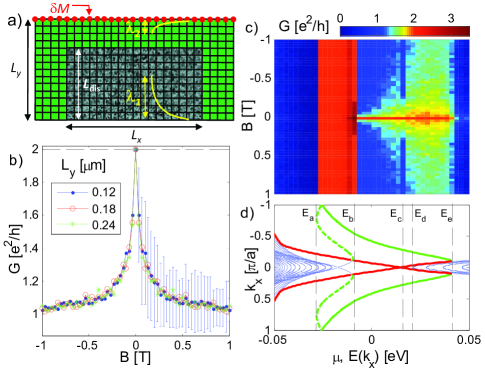
Figure 1: Magnetoconductance $G$ of a QSH edge: a) TB model with asymmetric edge states $\lambda_{2}\ll\lambda_{1}$ to study a single disordered edge; b) dependence of $G$ on sample width $L_{y}$ for disorder strength $W=55$ meV larger than the bulk gap, length $L_{x}=2.4\,\mu$m, fixed clean width $L_{y}-L_{\mathrm{dis}}=0.03\,\mu$m, and local mass term $\delta M=-70$ meV, with error bars (plotted for $L_{y}=0.12\,\mu$m and $B>0$ only) corresponding to conductance fluctuations $\delta G$; c) dependence of $G$ on chemical potential $\mu$; d) quasi-1D spectrum of the device illustrated in a) for zero $W,B$, showing bulk states (blue), top edge states (green) and bottom edge states (red).

We calculate numerically the $T=0$ disordered-averaged two-terminal conductance $G$ and conductance fluctuations $\delta G$ of a finite QSH strip (Fig. 1a) using the standard TB Green function approachFerry and Goodnick (1997). We find that $N_{\mathrm{dis}}\sim 100$ disorder configurations are enough to achieve good convergence for $G$ and $\delta G$. For a strip of width $L_{y}$ comparable to the edge state penetration depth $\lambda$, interedge tunnelingZhou et al. (2008) backscatters the edge states even at $B=0$ and the system is analogous to a topologically trivial quasi-1D quantum wire. To ensure that we are studying effects intrinsic to the topologically nontrivial QSH helical edge liquid, we first need to suppress interedge tunneling. The naive way to achieve this is to use a very large $L_{y}$; however, this can be computationally rather costly. We use a geometry (Fig. 1a) which allows us to effectively circumvent this problem while keeping $L_{y}$ reasonable. By adding a local Dirac mass termKönig et al. (2008) $\delta M<0$ on the first horizontal chain of our TB model (Fig. 1a, red dots), the penetration depth $\lambda_{2}$ at the top edge becomes much smaller than that at the bottom edge $\lambda_{1}\gg\lambda_{2}$. We then add disorder only to the last $L_{\mathrm{dis}}/a$ chains of the central region with $L_{\mathrm{dis}}\gg\lambda_{1}$ and $L_{y}-L_{\mathrm{dis}}\gg\lambda_{2}$. The resulting top edge states are very narrow, contribute an uninteresting background quantized conductance independent of $B$ and $W$, and are essentially decoupled from the bottom edge states (whose magnetoconductance we wish to study) that are effectively propagating in a semi-infinite disordered medium.

III Numerical Results

For $\mu$ inside the bulk gap, we expect edge transport to dominate the physics. The typical behavior of the magnetoconductance $G(B)$ for $\mathbf{B}=B\hat{\mathbf{z}}$ and disorder strength $W$ larger than the bulk gap $E_{g}\simeq 40$ meV is shown in Fig. 1b. The cusp-like feature at $B=0$ agrees qualitatively with the results of Ref. König et al., 2007. $G(B)$ is independent of $L_{y}$, which suggests that transport is indeed carried by the edge states. $G(B=0)$ is quantized to $G_{0}\equiv 2e^{2}/h$ independent of $W$ up to $W=71$ meV with extremely small conductance fluctuations $\delta G(B=0)/G_{0}\sim 10^{-5}$, which confirms that interedge tunneling is negligible even for strong disorder. Furthermore, $G$ tends to $G_{0}/2$ for large $|B|\sim 1$ T, which indicates that the disordered bottom edge is completely localized for large $W$ and $|B|$, and only the unperturbed top edge conducts. For $W<E_{g}$, $G$ is approximately quadratic in $B$ (not shown), and $|G(B)-G_{0}|/G_{0}\ll 1$ even for large $|B|\sim 1$ T. For $B\neq 0$, we observe that the amplitude of the fluctuations $\delta G$ does not decrease upon increasing $N_{\mathrm{dis}}$, and is roughly independent of $W$ with $\delta G/G_{0}\sim\mathcal{O}(10^{-1})$ for large enough disorder $W\gtrsim E_{g}$. Since in the absence of TRS the QSH system is a trivial insulator and the edge becomes analogous to an ordinary spinless 1D quantum wire with no topological protection, we conclude that $\delta G$ corresponds to the well-known universal conductance fluctuations Ferry and Goodnick (1997).

The dependence of $G(B)$ on $\mu$ is plotted in Fig. 1c. We consider $W=55$ meV slightly larger than $E_{g}$ (Fig. 1d). This is not unreasonable as the bulk mobility $\mu^{*}$ of the HgTe QW in Ref. König et al., 2007 is estimated as $\mu^{*}\simeq 10^{5}$ cm²/(V$\cdot$s), which corresponds to a momentum relaxation time $\tau=\mu^{*}m^{*}/e\simeq 0.57$ ps. The bulk carriers at the bottom of the conduction subband have an effective mass $m^{*}\simeq 0.01m_{e}$ where $m_{e}$ is the bare electron mass. $\tau$ is given by $\hbar/\tau\simeq 2\pi\nu(Wa)^{2}$, with $\nu$ the bulk continuum density of states at the Fermi energy given by $\nu\simeq m^{*}/\pi\hbar^{2}$. This yields $W\simeq 22$ meV. However, this estimate considers only bulk disorder and we expect edge roughness to yield a higher effective $W$ on the edge. Furthermore, this estimate is perturbative in $W$ and neglects interband effects which are expected to occur for $W\sim E_{g}$. For the chosen value of $W$ we observe that the bulk states (Fig. 1d, blue lines) are strongly localized with $G\ll G_{0}$ for $\mu<E_{a}$ and $\mu>E_{e}$ in the bulk bands, while the cusp-like feature at $B=0$ with $G(B=0)=G_{0}$ remains prominent for $E_{b}<\mu<E_{d}$ in the bulk gap and even at the bottom of the conduction band $E_{d}<\mu<E_{e}$ where the top edge states (Fig. 1d, red lines) coexist with the bulk states. The sudden dip in $G(B\neq 0)$ for $\mu\sim E_{c}\simeq 15$ meV corresponds to the opening of the small edge gap discussed earlier. Finally, $G\simeq G_{0}$ is almost independent of $B$ for $E_{a}<\mu<E_{b}$, where the disordered bottom edge and bulk states are mostly localized while the clean top edge supports another channel (Fig. 1d, dashed green line), with a total top edge conductance of $G=G_{0}$.

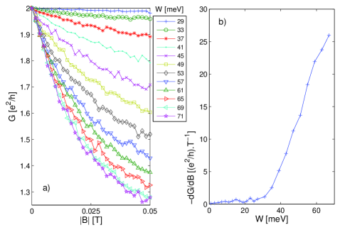
Figure 2: a) Magnetoconductance for various disorder strengths $W$; b) small-$B$ slope of the magnetoconductance (obtained by linear regression for $0<B<15$ mT). Device size is $(L_{x}\times L_{y})=(2.4\times 0.12)\,\mu$m².

The magnetoconductance for $B=B_{z}$ and various values of $W$ is plotted in Fig. 2. Although not evident from the figure, $G(B)$ is approximately quadratic in $B$ for $W<E_{g}$, and approximately linear in $|B|$ at small $B$ for $W>E_{g}$ (Fig. 2a). The slope of $G(B)$ at small fields (obtained by linear regression for $0<B<15$ mT where the dependence is approximately linear) is plotted in Fig. 2b, and is seen to increase rapidly for $W\gtrsim E_{g}\simeq 40$ meV. For $B=0$, we have essentially $G=G_{0}$ independent of $W$ (Fig. 2a). This contrasts with the results of Ref. Sheng et al., 2006; Li et al., 2009 where deviations from $G=G_{0}$ at $B=0$ occur for $W$ larger than some critical value $W_{c}>E_{g}$. The reason for this difference is that in Ref. Sheng et al., 2006; Li et al., 2009, disorder-induced collapse of the bulk gap is accompanied by the edge states penetrating deeper into the bulk and eventually reaching the opposite edge, such that interedge tunneling takes place and causes backscattering. Here, due to our special geometry (Fig. 1a) the top edge state is unperturbed and always remains localized near the edge, out of reach of the bottom edge state, even as the latter penetrates deeper into the disordered bulk for increasing $W$.

The BIA term $\Delta_{\mathbf{k}}$ has an important effect on $G$ for $B=B_{z}$ (Fig. 3a). For simplicity, we set $\Delta_{e}=\Delta_{h}=0$ and consider only the effect of $\Delta_{z}$. For $\Delta_{z}=0$, the perturbation $\mathcal{H}^{\prime}=e\mathbf{j}\cdot\mathbf{A}$ due to an orbital field, with $e$ the electron charge and $\mathbf{j}$ the current operator, has no matrix element between the spin states of a counterpropagating Kramers pair on a given edge König et al. (2008), and $G$ is unaffected. For an in-plane field, $H_{Z\parallel}$ does have a nonzero matrix element between these states, and there is a nontrivial magnetoconductance even in the absence of BIA.

The dependence of $G(B)$ on the orientation of $\mathbf{B}$ is plotted in Fig. 3b. The $g$-factorsRothe et al. (2010) used in the Zeeman terms are such that the Zeeman energies for in-plane and out-of-plane fields are of the same orderKönig et al. (2008). The in-plane vs out-of-plane anisotropy (Fig. 3b, $x,y$ vs $z$) arises from the orbital effect of the out-of-plane field $B=B_{z}$, which is absent for an in-plane field. In our model, the in-plane anisotropy is very weak (somewhat visible on Fig. 3b for $|B|\sim 1$ T), and is due to the inequivalence between the transport $x$ and confinement $y$ directions. Finally, the $B=0$ peak in $G$ is more pronounced for a smaller mass term $M$König et al. (2008) in the Dirac Hamiltonians $H_{\mathbf{k}},H^{*}_{-\mathbf{k}}$ (Fig. 3c). Since $E_{g}\propto|M|$ approximately, a smaller $|M|$ results in a larger dimensionless disorder strength $W/E_{g}$, which is equivalent to an increase in $W$ (see Fig. 2b).

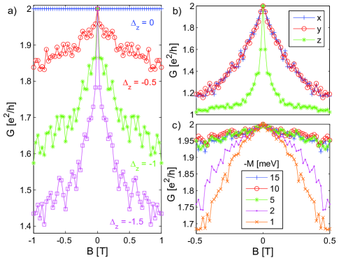
Figure 3: Dependence of the magnetoconductance $G$ on a) strength of the $\mathbf{k}$-independent BIA term $\Delta_{z}$ with $\Delta_{e}=\Delta_{h}=0$; b) magnetic field orientation; c) Dirac mass term $M<0$. Sample size is $(L_{x}\times L_{y})=(2.4\times 0.12)\,\mu$m², disorder strength is $W=55$ meV for a),b) and $W=30$ meV for c).

Although the mechanism behind the observed negative magnetoconductance $\Delta G\propto-|B|$ (Fig. 1,2) for an orbital field $B=B_{z}$ cannot be unambiguously inferred from our numerical results, a dependence linear in $|B|$ for small $B$ and the requirement of ‘strong’ disorder $W\gtrsim E_{g}$ for its observation seem to indicate that the effect has a nonperturbative character. A treatment which is perturbative in $W$ and $B$ yields at most, to leading order, the result $-\Delta G\propto\ell^{-1}\propto W_{\mathrm{eff}}^{2}(B)\propto B^{2}$, where $\ell$ is the mean free pathLee and Ramakrishnan (1985) and $W_{\mathrm{eff}}(B)\equiv W|B|/B_{0}$ is some effective disorder strength, with $B_{0}^{-1}\propto\Delta_{z}$ if only the effect of $\Delta_{z}$ is considered for simplicity. For ‘weak’ disorder $W<E_{g}$, the 1D edge states which enclose a negligible amount of flux are the only low-energy degrees of freedom, and the magnetic field only has a perturbative effect on them. Indeed, if we choose the gauge $\mathbf{A}=\bigl{(}B_{z}(L_{y}-y),0\bigr{)}$, for sufficiently small $B_{z}$ we have that $\mathbf{A}$ is small for $L_{y}-\lambda_{1}\lesssim y<L_{y}$ with $\lambda_{1}\ll L_{y}$ where the bottom edge state wavefunction has finite support (Fig. 1a), and the effect of an orbital field $B_{z}$ on a single edge can be treated perturbatively. In this case, the amplitude $\propto W_{\mathrm{eff}}(B)$ in perturbation theory for a leading order backscattering process on a single edge involves one power of $\Delta_{z}$ and one power of $B_{z}$ to couple the spin states of the counterpropagating Kramers partnersKönig et al. (2008) (with no momentum transfer as our choice of gauge preserves translational symmetry in the $x$ direction), and one power of $W$ to provide the necessary momentum transfer for backscattering. Our observation that $\Delta G\propto-B^{2}$ for $W<E_{g}$ corroborates this physical picture. On the other hand, the cusp-like feature at $B=0$ (Fig. 1b) occurs for ‘strong’ disorder $W\gtrsim E_{g}$, which seems to indicate that the bulk states play an important role. This leads us to a different physical picture. For $W\gtrsim E_{g}$, the edge electrons easily undergo virtual transitions to the bulk. In other words, the emergent low-energy excitations for $W\gtrsim E_{g}$ extend deeper into the bulk than the ‘bare’ edge electrons. The electrons spend a significant amount of time diffusing randomly in the bulk away from the edge, with their trajectories enclosing finite amounts of flux before returning to the edge, which endows the orbital field with a nonperturbative effect. In this way the conventional picture of 2D antilocalization (AL)Bergmann (1984) can apply, at least qualitatively, to a single disordered QSH edge. We are thus led to the interesting picture, peculiar to the QSH state, of a dimensional crossover between 1D AL Zirnbauer (1992); Tak in the weak disorder regime $W<E_{g}$ with the orbital field having a perturbative effect, to an effect analogous to 2D AL in the strong disorder regime $W>E_{g}$ with the orbital field having a nonperturbative effect.

IV Conclusion

We have shown that ‘strong’ disorder effects $W/E_{g}\sim 1$ in a QSH insulator in the presence of a magnetic field $B$ and inversion symmetry breaking terms can give rise to a cusp-like feature in the two-terminal edge magnetoconductance with an approximate linear dependence $\Delta G(B)\propto-|B|$ for small $B$. These results are in good qualitative agreement with experiments. A possible physical intepretation of our results consists of a dimensional crossover scenario where a weakly disordered, effectively spinless 1D edge liquid crosses over, for strong enough disorder, to a state where disorder enables frequent excursions of the edge electrons into the disordered flux-threaded 2D bulk, resulting in a behavior reminiscent of 2D AL.

We wish to thank M. König, H. Buhmann, L. W. Molenkamp, E. M. Hankiewicz, C. X. Liu, T. L. Hughes, R. D. Li, H. Yao, and M. Bourbonniere for insightful discussions. This work was supported by the Department of Energy, Office of Basic Energy Sciences, Division of Materials Sciences and Engineering, under contract DE-AC02-76SF00515. JM acknowledges support from the National Science and Engineering Research Council of Canada, the Fonds Québécois de la Recherche sur la Nature et les Technologies, and the Stanford Graduate Fellowship program. Computational work was made possible by the computational resources of the Stanford Institute for Materials and Energy Science, and those of the Shared Hierarchical Academic Research Computing Network (www.sharcnet.ca).

References

- Bernevig et al. (2006) B. A. Bernevig, T. L. Hughes, and S. C. Zhang, Science 314, 1757 (2006).
- König et al. (2007) M. König, S. Wiedmann, C. Brüne, A. Roth, H. Buhmann, L. W. Molenkamp, X. L. Qi, and S. C. Zhang, Science 318, 766 (2007).
- Roth et al. (2009) A. Roth, C. Brüne, H. Buhmann, L. W. Molenkamp, J. Maciejko, X. L. Qi, and S. C. Zhang, Science 325, 294 (2009).
- Büttiker (2009) M. Büttiker, Science 325, 278 (2009).
- Kane and Mele (2005) C. L. Kane and E. J. Mele, Phys. Rev. Lett. 95, 146802 (2005).
- Bernevig and Zhang (2006) B. A. Bernevig and S. C. Zhang, Phys. Rev. Lett. 96, 106802 (2006).
- König et al. (2008) M. König, H. Buhmann, L. W. Molenkamp, T. Hughes, C. X. Liu, X. L. Qi, and S. C. Zhang, J. Phys. Soc. Jpn 77, 031007 (2008).
- Wu et al. (2006) C. Wu, B. A. Bernevig, and S. C. Zhang, Phys. Rev. Lett. 96, 106401 (2006).
- Xu and Moore (2006) C. Xu and J. E. Moore, Phys. Rev. B 73, 045322 (2006).
- Qi et al. (2008) X. L. Qi, T. L. Hughes, and S. C. Zhang, Nature Phys. 4, 273 (2008).
- Tkachov and Hankiewicz (2010) G. Tkachov and E. M. Hankiewicz, Phys. Rev. Lett. 104, 166803 (2010).
- M. König (2007) M. König, Ph.D. thesis, University of Würzburg (2007).
- Sheng et al. (2006) D. N. Sheng, Z. Y. Weng, L. Sheng, and F. D. M. Haldane, Phys. Rev. Lett. 97, 036808 (2006).
- Onoda et al. (2007) M. Onoda, Y. Avishai, and N. Nagaosa, Phys. Rev. Lett. 98, 076802 (2007).
- Obuse et al. (2007) H. Obuse, A. Furusaki, S. Ryu, and C. Mudry, Phys. Rev. B 76, 075301 (2007).
- Li et al. (2009) J. Li, R.-L. Chu, J. K. Jain, and S.-Q. Shen, Phys. Rev. Lett. 102, 136806 (2009).
- Li and Shi (2009) D. Li and J. Shi, Phys. Rev. B 79, 241303(R) (2009).
- Maciejko et al. (2009) J. Maciejko, C. X. Liu, Y. Oreg, X. L. Qi, C. Wu, and S. C. Zhang, Phys. Rev. Lett. 102, 256803 (2009).
- Rothe et al. (2010) D. G. Rothe, R. W. Reinthaler, C. X. Liu, L. W. Molenkamp, S. C. Zhang, and E. M. Hankiewicz, New J. Phys. 12, 065012 (2010).
- Winkler (2003) R. Winkler, Spin-Orbit Coupling Effects in Two-Dimensional Electron and Hole Systems (Springer-Verlag, Berlin, 2003).
- Ferry and Goodnick (1997) D. K. Ferry and S. M. Goodnick, Transport in Nanostructures (Cambridge University Press, Cambridge, 1997).
- Zhou et al. (2008) B. Zhou, H.-Z. Lu, R.-L. Chu, S.-Q. Shen, and Q. Niu, Phys. Rev. Lett. 101, 246807 (2008).
- Lee and Ramakrishnan (1985) P. A. Lee and T. V. Ramakrishnan, Rev. Mod. Phys. 57, 287 (1985).
- Bergmann (1984) G. Bergmann, Phys. Rep. 107, 1 (1984).
- Zirnbauer (1992) M. R. Zirnbauer, Phys. Rev. Lett. 69, 1584 (1992).
- (26) Y. Takane, J. Phys. Soc. Jpn. 73, 1430 (2004); 73, 2366 (2004).