Non-Gaussianity in WMAP 5-year CMB map seen through Needlets

Abstract

The cosmic microwave background radiation is supposed to be Gaussian and this hypothesis is in good agreement with the recent very accurate measurements. Nonetheless a tiny amount of non-Gaussianity is predicted by the standard inflation scenario, while more exotic models suggest a higher degree of non-Gaussianity. Tightly constraining the level of Gaussianity in the CMB data represents then a fundamental handle to understand the physics and the origin of our universe. By means of needlets, a novel rendition of wavelets, characterised by excellent properties of localisations both in harmonic and pixel domain, we are able to detect anomalous spots in the southern hemisphere responsible for roughly the 50% of power asymmetry we measure in the CMB power spectrum, and to perform a detailed analysis of the needlets bispectrum. We then constrain the primordial non-Gaussianity parameter, $f_{\rm NL}=21\pm 40$ at 68% c.f., and spot a high asymmetry in the bispectrum, in particular in the isosceles configurations.

1 Introduction

During the last decade the quality of the cosmological observations has increased impressively, providing theorists with very accurate datasets. Cosmic Microwave Background radiation (CMB) measurements (Hinshaw et al., 2009), SuperNovae IA (Riess et al., 2009) and Baryonic Acoustic Oscillations (Percival et al., 2009) fit pretty well within the scenario of the so-called Cosmological Concordance Model ($\Lambda$CDM), which describes fairly well the evolution of the Universe by means of an handful of parameters (Komatsu et al., 2009). We live in a flat universe, whose critical density is provided by baryons $\Omega_{\rm b}\simeq 4\%$, dark matter $\Omega_{\rm c}\simeq 25\%$, responsible for the structures formation, and the troublesome vacuum energy, $\Omega_{\Lambda}\simeq 70\%$. The other parameters set the normalisation, $A_{\rm s}$, and the power, $n_{\rm s}$, of the primordial cosmological fluctuations and the contribution of the stars formation at more recent epoch, $\tau$. Despite its simplicity, the $\Lambda$CDM model lacks of a solid theoretical basis. The value and the origin of the vacuum energy is far from being understood (Copeland et al., 2006), and the mechanism which seeds the cosmological perturbations, namely inflation (Guth, 1981), remains more a scenario than a full tested theory. Our Universe is supposed to be homogeneous and isotropic with nearly Gaussian fluctuations. Indeed this is in good agreement with the most recent data, even though the mechanism generating the perturbations itself should introduce a small non-Gaussian contribution (Bartolo et al., 2004). Moreover, exotic early universe scenarios, such as brane-inspired models (Steinhardt & Turok, 2002), multi-fields (Lyth & Wands, 2002) or ekpyrotic models (Mizuno et al., 2008) predict a higher level of non-Gaussianity. Accurately determining the statistics of the cosmological perturbations represents a fundamental handle on the early universe physics necessary for understanding the nature and the evolution of our Universe.

In the following we tackle the issue of non-Gaussianity in the CMB data, analysing the WMAP 5-year temperature data by means of needlets. Needlets are a novel rendition of wavelets introduced first in functional analysis (Narcowich et al., 2006) and then extended to statistical (Baldi et al., 2006) and CMB data analysis (Pietrobon et al., 2006). Needlets are a basis (more properly a tight frame) defined directly on the sphere, which shows an exponential localisation property both in pixel and harmonic space. Moreover they are very weakly correlated: this makes them particularly suitable for CMB data analysis where partial sky coverage, noise and beam effects have to be minimised in order to extract tiny signals, especially when non-Gaussian. Needlets are a quadratic combination of spherical harmonics, weighted by a window function, $b(\ell/B^{j})$

$$\psi_{jk}(\hat{\gamma})=\sqrt{\lambda_{jk}}\sum_{\ell}b\Big{(}\frac{\ell}{B^{j}}\Big{)}\sum_{m=-\ell}^{\ell}\overline{Y}_{\ell m}(\hat{\gamma})Y_{\ell m}(\xi_{jk}),$$ (1)

where $\hat{\gamma}$ represents a direction in the sky, $\{\xi_{jk}\}$ is a set of cubature points (for practical purpose identified with a pixelization of the sphere (Górski et al., 2005)), and $B$ a user chosen parameter which determines the filter width in harmonic space. For a detailed discussion see Marinucci et al. (2008) and refs.  therein. An example of this filter is given in Fig. 1, together with the needlet profile in real space. The localisation property is clearly visible.

Figure 1: Profile of the $b(\ell/B^{j})$ filter (top) and needlet (bottom) for the choice $B=1.8$ $j=4$.

2 Spot detection and Power spectrum asymmetry

Since the first release, the WMAP data have been tested against Gaussianity and asymmetry (see e.g. Eriksen et al. (2004); Cruz et al. (2005); Land & Magueijo (2007); de Oliveira-Costa et al. (2004)). We applied needlets to the 5-year data to study the anomaly/asymmetry problem in a coherent framework. We extracted the needlets coefficients from the temperature map given by

$$\beta_{jk}=\sum_{\ell}b\left(\frac{\ell}{B^{j}}\right)\sum_{m}a_{\ell m}Y_{\ell m}(\xi_{jk}).$$

$\beta_{jk}$ can be easily represented in a mollweide projection: the case of the Internal Linear Combination map is given in Fig. 2.

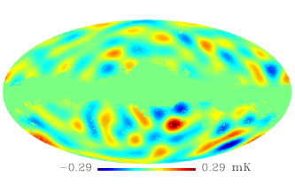
Figure 2: Needlet coefficients of the WMAP 5-year CMB temperature map. $B=1.8$ and $j=4$.

Notice that needlets coefficients are analytically linked to those of the spherical harmonics: this guarantees an expression for the 2- and 3-point correlation functions, respectively the power spectrum and bispectrum. By applying needlets, we found three very significant spots in the southern hemisphere (the brightest features in Fig. 2) which seem to be barely compatible with the Gaussian hypothesis (Pietrobon et al., 2008). Thanks to needlets localisation, we were able to determine which angular scales they span. In particular computing the needlets power spectrum

$$\beta_{j}\equiv\frac{1}{N_{\rm pix}}\sum_{k}\beta_{jk}^{2}=\sum_{\ell}b^{2}\Big{(}\frac{\ell}{B^{j}}\Big{)}\frac{2\ell+1}{4\pi}C_{\ell},$$ (2)

where $C_{\ell}=\langle|a_{\ell m}|^{2}\rangle$, we found that the significant power asymmetry between the north and the south hemisphere is localised at large scales, where the spots peak. Moreover, masking the spots, we measured a decrease of the difference in power of a factor 2, underlining the substantial contribution given by these anomalous features. Fig. 3 summarises our results. We checked whether this effect influences the parameter estimation, finding that, with the current precision, the difference remains within one sigma.

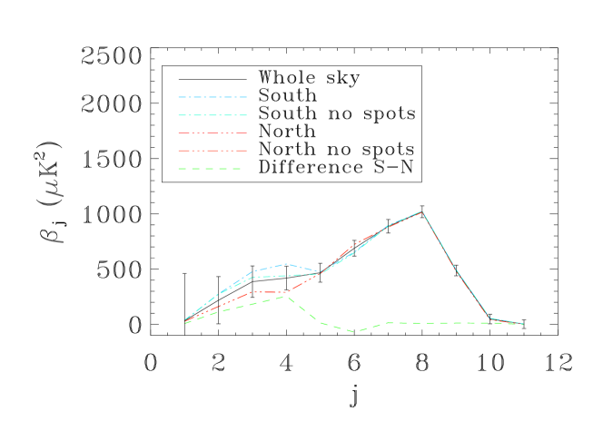
Figure 3: $\beta_{j}$ extracted from WMAP data for different sky cuts. The black solid line shows the signal for the whole CMB sky (kq85 is applied). The blue and red dashed lines show how the power is split between the two hemispheres. When the cold and hot spots detected are masked the excess of power in the southern region is decreased (light blue and orange dot-dashed lines).

3 Bispectrum analysis

The signature of non-Gaussianity appears in the higher moments of a distribution, which are no longer completely specified by the first moment (i.e. the mean value of the distribution) and the second moment (i.e. the standard deviation). For a Gaussian distribution, all odd moments are vanishing, while the even ones can be expressed in term of just the first two. We then look for a non-vanishing bispectrum of the distribution of the needlets coefficients. The amplitude of the bispectrum is usually parameterised by the non-linear parameter $f_{\rm NL}$ which governs the amplitude of the non-Gaussian contribution to the primordial gravitational potential expansion with respect to the linear leading bit:

$$\Phi(x)=\Phi_{\rm L}(x)+f_{\rm NL}\left[\Phi^{2}_{\rm L}(x)-\langle\Phi_{\rm L}^{2}(x)\rangle\right].$$ (3)

The primordial fluctuations are converted into CMB ones, whose bispectrum is given by $\langle a_{\ell_{1}m_{1}}a_{\ell_{2}m_{2}}a_{\ell_{3}m_{3}}\rangle$. In needlets space the former expression reads:

$$S_{j_{1}j_{2}j_{3}}=\frac{1}{N_{\rm pix}}\sum_{k}\frac{\beta_{j_{1}k}\beta_{j_{2}k}\beta_{j_{3}k}}{\sigma_{j_{1}}\sigma_{j_{2}}\sigma_{j_{3}}},$$ (4)

where $N_{\rm pix}$ is the number of pixels outside the applied mask and $\sigma_{j}$ the variance of the needlets coefficient at the $j$ resolution. See Pietrobon et al. (2009) and Refs.  therein for a detailed discussion. We extracted needlets coefficients from the noise weighted combination of the WMAP5 channels and measured $f_{\rm NL}$ by applying the following estimator (Pietrobon et al., 2009):

$$f_{\rm NL}=\frac{\sum_{jj^{\prime}}S^{\rm obs}_{j}\mathbf{Cov}^{-1}_{jj^{\prime}}S^{\rm th}_{j^{\prime}}}{\sum_{jj^{\prime}}S^{\rm th}_{j}\mathbf{Cov}^{-1}_{jj^{\prime}}S^{\rm th}_{j^{\prime}}}.$$ (5)

We obtained $f_{\rm NL}=21\pm 40$ at 68% c.l. We calibrated our result by means of both Gaussian and non-Gaussian (Liguori et al., 2007) simulations of the underlying $\Lambda$CDM best fit model. Our constraints are consistent with those obtained with different techniques: having several tools, affected by different systematics, is crucial for analysing the upcoming cosmological experiments datasets.

The $f_{\rm NL}$ parameter encodes all the information contained in the bispectrum irrespective of the specific triangle configuration. The bispectrum signal can be actually split according to the geometry in equilateral, isosceles, scalene and open configurations. Different kinds of non-Gaussianity may result in different shapes, so it is worth looking at them separately. This is what we addressed in Pietrobon et al. (2009). The main result of the paper is summarised in Tab. 1, where the percentage of random Gaussian simulations with a $\chi^{2}$ higher than the data is quoted.

conf.	FULL SKY	NORTH	SOUTH
all (115)	$29\%$	$\mathbf{96\%}$	$\mathbf{2\%}$
equi (9)	$20\%$	$11\%$	$45\%$
iso (56)	$5\%$	$\mathbf{96\%}$	$\mathbf{0.5\%}$
scal (50)	$60\%$	$\mathbf{90\%}$	$\mathbf{7\%}$
open (50)	$3\%$	$\mathbf{85\%}$	$\mathbf{2\%}$

Table 1: Percentage of the simulations with a $\chi^{2}$ larger than WMAP 5-year data for the different triangular configurations of the needlets bispectrum.

Again, the southern hemisphere results very anomalous, especially in the isosceles configurations, those characterised by a local type of non-Gaussianity.

4 Conclusions

We have discussed the importance of characterising the statistical distribution of the cosmological perturbations to understand the early universe physics. We study in detail several properties of the CMB sky where a non-Gaussian signal may arise by means of needlets. We found anomalous spots in the southern hemisphere which account for the 50% of the power spectrum asymmetries. Moreover we measured the needlets bispectrum constraining the primordial non-Gaussianity parameter and studying its properties according to the geometry of the triangle configurations. The isosceles ones turn out to be the most anomalous: whether this is a signature of a peculiar early universe model is an interesting issue in light of the new upcoming experiments.

References

- Baldi et al. (2006) Baldi, P. et al. 2006, Annals of Statistics 2009, Vol. 37, No. 3, 1150-1171
- Bartolo et al. (2004) Bartolo, N. et al. 2004, Phys. Rep., 402, 103
- Copeland et al. (2006) Copeland, E. J. et al. 2006, Int. J. Mod. Phys., D15, 1753
- Cruz et al. (2005) Cruz, M. et al. 2005, MNRAS, 356, 29
- de Oliveira-Costa et al. (2004) de Oliveira-Costa, A. et al. 2004, Phys. Rev. D, 69, 063516
- Eriksen et al. (2004) Eriksen, H. K. et al. 2004, ApJ, 609, 1198
- Górski et al. (2005) Górski, K. M. et al. 2005, ApJ, 622, 759
- Guth (1981) Guth, A. H. 1981, Phys. Rev. D, 23, 347
- Hinshaw et al. (2009) Hinshaw, G. et al. 2009, ApJS, 180, 225
- Komatsu et al. (2009) Komatsu, E. et al. 2009, ApJS, 180, 330
- Land & Magueijo (2007) Land, K. & Magueijo, J. 2007, MNRAS, 378, 153
- Liguori et al. (2007) Liguori, M. et al. 2007, Phys. Rev. D, 76, 105016
- Lyth & Wands (2002) Lyth, D. H. & Wands, D. 2002, Phys. Lett. B, 524, 5
- Marinucci et al. (2008) Marinucci, D., Pietrobon, D., et al. 2008, MNRAS, 383, 539
- Mizuno et al. (2008) Mizuno, S. et al. 2008, in American Institute of Physics Conference Series, Vol. 1040, 121–125
- Narcowich et al. (2006) Narcowich, F. J., Petrushev, P., & Ward, J. D. 2006, SIAM J. Math. Anal., 38, 574
- Percival et al. (2009) Percival, W. J. et al. 2009, arXiv: 0907.1660
- Pietrobon et al. (2006) Pietrobon, D. et al. 2006, Phys. Rev. D, 74, 043524
- Pietrobon et al. (2008) Pietrobon, D. et al. 2008, Phys. Rev. D, 78, 103504
- Pietrobon et al. (2009) Pietrobon, D. et al. 2009, MNRAS, 396, 1682
- Pietrobon et al. (2009) Pietrobon, D. et al. 2009, arXiv: 0905.3702
- Riess et al. (2009) Riess, A. G. et al. 2009, ApJ, 699, 539
- Steinhardt & Turok (2002) Steinhardt, P. J. & Turok, N. 2002, Science, 296, 1436