The Chandra Deep Protocluster Survey: Point-Source Catalogs for a 400 ks Observation of the z = 3.09 Protocluster in SSA22.

Abstract

We present X-ray point-source catalogs for a deep $\approx$400 ks Chandra ACIS-I exposure of the SSA22 field. The observations are centred on a $z=3.09$ protocluster, which is populated by Lyman break galaxies (LBGs), Ly$\alpha$ emitters (LAEs), and extended Ly$\alpha$-emitting blobs (LABs). The survey reaches ultimate (3 count) sensitivity limits of $\approx$5.7 $\times 10^{-17}$ ergs cm^-2 s^-1 and $\approx$3.0 $\times 10^{-16}$ ergs cm^-2 s^-1 for the 0.5–2 keV and 2–8 keV bands, respectively (corresponding to $L_{\rm 2-10~{}keV}\approx 5.7\times 10^{42}$ and $L_{\rm 10-30~{}keV}\approx 2.0\times 10^{43}$ ergs s^-1 at $z=3.09$, respectively, for an assumed photon index of $\Gamma=1.4$). These limits make SSA22 the fourth deepest extragalactic Chandra survey yet conducted, and the only one focused on a known high redshift structure. In total, we detect 297 X-ray point sources and identify one obvious bright extended X-ray source over a $\approx$330 arcmin² region. In addition to our X-ray catalogs, we provide all available optical spectroscopic redshifts and near-infrared and mid-infrared photometry available for our sources. The basic X-ray and infrared properties of our Chandra sources indicate a variety of source types, although absorbed active galactic nuclei (AGNs) appear to dominate. In total, we have identified 12 X-ray sources (either via optical spectroscopic redshifts or LAE selection) at $z=$ 3.06–3.12 that are likely to be associated with the SSA22 protocluster. These sources have X-ray and multiwavelength properties that suggest they are powered by AGN with 0.5–8 keV luminosities in the range of $\approx$$10^{43}$–$10^{45}$ ergs s^-1. We have analysed the AGN fraction of sources in the protocluster as a function of local LAE source density and find suggestive evidence for a correlation between AGN fraction and local LAE source density (at the $\approx$96 per cent confidence level), implying that supermassive black hole growth at $z\approx 3$ is strongest in the highest density regions.

1 Introduction

Deep X-ray surveys with Chandra and XMM-Newton have provided a unique perspective on the cosmic evolution of accreting supermassive black holes (SMBHs) and high-energy activity from normal galaxies (e.g., star-formation processes, evolving stellar binaries, and hot gas cooling) over significant fractions of cosmic history (see Fig. 1 and Brandt & Hasinger 2005 for a review). Due to limitations originating from point-source confusion for XMM-Newton at 0.5–2 keV flux levels below $\approx$$10^{-16}$ ergs cm^-2 s^-1, the deepest views of the extragalactic X-ray Universe have come exclusively from deep Chandra surveys with exposures $\;\buildrel>\over{\sim}\;$200 ks.

The deepest Chandra surveys to date are the $\approx$2 Ms Chandra Deep Field-North (CDF-N; Alexander et al. 2003) and $\approx$2 Ms Chandra Deep Field-South (CDF-S; Luo et al. 2008) surveys (hereafter, the Chandra Deep Fields; CDFs). These have been supplemented by additional deep Chandra surveys (e.g., the $\approx$250 ks Extended CDF-S [E-CDF-S; Lehmer et al. 2005] and the 0.2–0.8 Ms Extended Groth Strip [AEGIS-X; Laird et al. 2009]), which cover larger solid angles than the CDFs and provide important X-ray information on rarer source populations. These deep Chandra surveys have been chosen to lie at high Galactic latitudes in regions of the sky that have relatively low Galactic columns ($\;\buildrel<\over{\sim}\;$10²⁰ cm^-2) and few local sources in the field, as to gain a relatively unobscured and unbiased perspective of the distant ($z\lower 2.15277pt\hbox{$\;\buildrel>\over{\sim}\;$}0.1$) Universe. Despite these growing resources, there has not yet been an equivalent survey targeting very high-density regions of the $z\lower 2.15277pt\hbox{$\;\buildrel>\over{\sim}\;$}2$ Universe where the most massive SMBHs and galaxies are thought to be undergoing very rapid growth (e.g., Kauffmann 1996; De Lucia et al. 2006). In order to address this limitation and study the growth of SMBHs and galaxies as a function of environment, we have carried out a deep $\approx$400 ks Chandra survey (PI: D. M. Alexander) of the highest density region in the $z=3.09$ SSA22 protocluster.

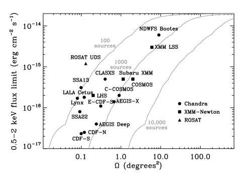
Figure 1: Locations of some well-known extragalactic X-ray surveys conducted with Chandra (circles), XMM-Newton (squares), and ROSAT (triangles) in the 0.5–2 keV flux limit versus solid-angle $\Omega$ plane. Each survey has a range of flux limits across its solid angle; we have generally shown the most sensitive flux limit. This plot has been adapted from Fig. 1 of Brandt & Hasinger (2005) to show the part of parameter space most relevant for SSA22; see Table 1 of Brandt & Hasinger (2005) for references and descriptions of many of the surveys plotted here. The gray curves show contours regions of the flux limit versus solid angle plane where $\approx$100, 1000, and 10,000 sources are expected to be detected (based on the Bauer et al. 2004 number counts relation).

The $z=3.09$ SSA22 protocluster was originally identified by Steidel et al. (1998), who found a significant overdensity ($\approx$4–6 times higher surface density than the field) within an $\approx$$8\times 8$ arcmin² region ($\approx$$15\times 15$ comoving Mpc² at $z=3.09$) through spectroscopic follow-up observations of $z\sim 3$ candidate Lyman break galaxies (LBGs). Theoretical modelling indicates that the protocluster will evolve into a rich cluster with a total mass $\;\buildrel>\over{\sim}\;$$10^{15}$ $M_{\odot}$ at the present day (e.g., Coma; see Steidel et al. 1998 for details). Since its discovery, the protocluster has also been found to contain a factor of $\approx$6 overdensity of Ly$\alpha$ emitters (LAEs; Steidel et al. 2000; Hayashino et al. 2004; Matsuda et al. 2005) and many remarkable bright extended Ly$\alpha$-emitting blobs (LABs; Steidel et al. 2000; Matsuda et al. 2004), which are believed to be sites of massive galaxy formation powered by starburst/AGN outflows (e.g., Bower et al. 2004; Geach et al. 2005, 2009; Wilman et al. 2005). Therefore, SSA22 is an ideal field for studying how SMBH growth depends on environment in the $z\gg$ 1 Universe.

In addition to the LBG and LAE surveys, SSA22 has become a premier multiwavelength survey field. The region has been imaged from space by HST in a sparse mosaic of 12 ACS pointings using the F814W filter and by Spitzer over the entire field in four IRAC bands (3.6, 4.5, 5.8, and 8.0$\mu$m) and at 24$\mu$m by MIPS (see Fig. 2). Additionally, the ground-based observations are extensive and include imaging at radio (1.4 GHz from the VLA; Chapman et al. 2004), submm (SCUBA 850$\mu$m, AzTEC 1.1mm, and LABOCA 870$\mu$m; Chapman et al. 2001; Geach et al. 2005; Tamura et al. 2009), near-infrared ($J$, $H$, and $K$ bands from UKIRT and Subaru; Lawrence et al. 2007; Uchimoto et al. 2008), and optical wavelengths (e.g., Subaru $B$, $V$, $R$, $i^{\prime}$, $z^{\prime}$, and NB497 bands; Hayashino et al. 2004). A variety of spectroscopic campaigns have been conducted (e.g., at Kitt Peak, Subaru, Keck, and the VLT; Steidel et al. 2003; Matsuda et al. 2005; Garilli et al. 2008; Chapman et al. 2009, in-preparation) and others are currently underway.

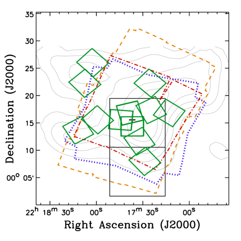
Figure 2: Coverage map of SSA22 showing Chandra (dotted blue polygon), HST (green solid squares), and Spitzer IRAC (orange short-dashed polygon) and MIPS (red dot-dashed polygon) observational regions. Additionally, we have highlighted the Steidel et al. (2003) LBG survey regions SSA22a and SSA22b (solid black rectangles) and LAE source-density contours are shown in gray (computed using LAEs from Hayashino et al. 2004 and a spatially-varying density extraction circle with radius of 3.0 arcmin) and have levels of 0.8, 1.1, 1.4, 1.7, and 2.0 LAEs arcmin^-2.

Thus far, we have utilised the Chandra and multiwavelength data presented here to conduct two scientific investigations including (1) Lehmer et al. (2009), which finds that the growth of galaxies and SMBHs in the $z=3.09$ protocluster environment is enhanced by a factor of $\approx$2–16 over that found in $z\approx 3$ field galaxies (i.e., in the CDFs), and (2) Geach et al. (2009), which uses the Chandra data to study the host galaxies of LABs and concludes that AGN and star-formation activity provide more than enough UV emission to power the extended Ly$\alpha$ emission. Additional follow-up investigations and scientific studies are planned and will be presented in subsequent papers.

In this paper, we present Chandra point-source catalogs and data products derived from the $\approx$400 ks SSA22 data set. The paper is orgainized as follows: In $\S$2, we provide details of the observations and data reduction. In $\S$3, we present Chandra point-source catalogs and details of our technical analyses. In $\S$4, we present basic multiwavlength properties of the X-ray sources and conduct scientific analyses of sources within the SSA22 protocluster. Finally, in $\S$5, we analyse the X-ray properties of the only obvious extended X-ray source in the field J221744.6+001738. The observational procedures and data processing were similar in spirit to those presented in Lehmer et al. (2005) and Luo et al. (2008); however, we have made wider use of the Chandra data analysis software package ACIS EXTRACT version 3.131 (Broos et al. 2002) while producing our point-source catalogs (see $\S$3 for further details).

Throughout this paper, we assume the Galactic column density along the line of sight to SSA22 to be $N_{\rm H}=4.6\times 10^{20}$ cm^-2 (e.g., Stark et al. 1992). The coordinates throughout this paper are J2000. $H_{0}$ = 70 km s^-1 Mpc^-1, $\Omega_{\rm M}$ = 0.3, and $\Omega_{\Lambda}$ = 0.7 are adopted throughout this paper (e.g., Spergel et al. 2003), which give the age of the Universe as 13.5 Gyr and imply a $z=3.09$ look-back time and spatial scale of 11.4 Gyr and 7.6 kpc arcsec^-1, respectively.

Table 1: Journal of SSA22 Chandra Observations

Obs.	Obs.	Exposure	Aim Point		Roll
ID	Start (UT)	Time (ks)a	$\alpha_{\rm J2000}$	$\delta_{\rm J2000}$	Angle (∘)b
9717………………	2007-10-01, 06:48	116.0	22 17 36.80	+00 15 33.09	280.2
8035………………	2007-10-04, 04:28	96.0	22 17 36.80	+00 15 33.10	280.2
8034………………	2007-10-08, 17:36	108.9	22 17 36.80	+00 15 33.10	280.2
8036………………	2007-12-30, 01:21	71.1	22 17 37.27	+00 15 38.37	297.9

^aAll observations were continuous. The short time intervals with bad satellite aspect are negligible and have not been removed. ^bRoll angle describes the orientation of the Chandra instruments on the sky. The angle is between 0–360^∘, and it increases to the West of North (opposite to the sense of traditional position angle). The total exposure time for the SSA22 observations is 392 ks and the exposure-weighted average aim point is $\alpha_{\rm J2000}=$ 22:17:36.8 and $\delta_{\rm J2000}=$ +00:15:33.1.

2 Observations and Data Reduction

2.1 Instrumentation and Observations

The ACIS-I camera (Garmire et al. 2003) was used for all of the SSA22 Chandra observations. The ACIS-I full field of view is $16.9\times 16.9$ arcmin² (i.e., $31.7\times 31.7$ comoving Mpc² at $z=3.09$), and the sky-projected ACIS pixel size is $\approx$$0.492$ arcsec ($\approx$3.8 kpc pixel^-1 at $z=3.09$). The point-spread function (PSF) is smallest at the lowest photon energies and for sources with small off-axis angles and increases in size at higher photon energies and larger off-axis angles. For example, the 95 per cent encircled-energy fraction radius at 1.5 keV at 0–8 arcmin off axis is $\approx 1.8$–$7.5$ arcsec (Feigelson et al. 2000; Jerius et al. 2000). The shape of the PSF is approximately circular at small off-axis angles, broadens and elongates at intermediate off-axis angles, and becomes complex at large off-axis angles.

The entire $\approx$400 ks Chandra exposure consisted of four separate Chandra observations of $\approx$70–120 ks taken between 2007 October 1 and 2007 December 30 and is summarised in Table 1. The four ACIS-I CCDs were operated in all of the observations; due to their large angular offsets from the aim point, the ACIS-S CCDs were turned off for all observations. All observations were taken in Very Faint mode to improve the screening of background events and thus increase the sensitivity of ACIS in detecting faint X-ray sources. Due to dithering and small variations in roll angles and aim points (see Table 1), the observations cover a total solid angle of 330.0 arcmin², somewhat larger than a single ACIS-I exposure (295.7 arcmin²). Combining the four observations gave a total exposure time of 392 ks and an exposure-weighted average aim point of $\alpha_{\rm J2000}=$ 22:17:36.8 and $\delta_{\rm J2000}=$ +00:15:33.1.

As discussed in $\S$1, the SSA22 Chandra target centre was chosen to coincide with the highest density regions of the $z=3.09$ SSA22 protocluster (see Fig. 2), where an additional $\approx$79 ks of ACIS-S imaging is already available (PI: G. Garmire). We experimented with source searching utilizing both the new $\approx$400 ks ACIS-I and previously available $\approx$79 ks ACIS-S observations and found that the number of detected sources was not significantly increased. To avoid the unnecessary complications of combining data with significantly different aim-points, backgrounds, and PSFs, we therefore chose to restrict our Chandra analyses to the $\approx$400 ks ACIS-I observations alone.

2.2 Data Reduction

Chandra X-ray Center (hereafter CXC) pipeline software was used for basic data processing, and the pipeline version 7.6.11 was used in all observations. The reduction and analysis of the data used Chandra Interactive Analysis of Observations (CIAO) Version 3.4 tools whenever possible; however, custom software, including the TARA package, was also used extensively.

Each level 1 events file was reprocessed using the CIAO tool acis_process_events to correct for the radiation damage sustained by the CCDs during the first few months of Chandra operations using the Charge Transfer Inefficiency (CTI) correction procedure of Townsley et al. (2000, 2002) and remove the standard pixel randomization. Undesirable grades were filtered using the standard ASCA grade set (ASCA grades 0, 2, 3, 4, 6) and known bad columns and bad pixels were removed using a customized stripped-down version (see $\S$2.2 of Luo et al. 2008 for additional details) of the standard bad pixel file. The customized bad-pixel file does not flag pixels that are thought to have a few extra events per Ms in the 0.5–0.7 keV bandpass. These events are flagged as bad pixels and removed in the standard CXC pipeline-reduced events lists; however, events landing on these pixels with energies above $\approx$0.7 keV are expected to be valid events. We therefore, chose to include these columns in our analyses.

After removing the bad pixels and columns, we cleaned the exposures of cosmic-ray afterglows and hot columns using the acis_detect_afterglow procedure. We found that the use of this procedure removed cosmic-ray afterglows more stringently than the acis_run_hotpix procedure used in the standard CXC reductions without removing any obvious real X-ray sources.

Background light curves for all four observations were inspected using EVENT BROWSER in the Tools for ACIS Real-time Analysis (TARA; Broos et al. 2000) software package. None of the observations had significant flaring events, defined by the background level being $\;\buildrel>\over{\sim}\;$1.5 times higher than nominal. We therefore did not filter any of the observations for flaring events.

We registered our observations to the astrometric frame of the UKIRT Infrared Deep Sky Survey (UKIDSS; e.g., Lawrence et al. 2007) Deep Extragalactic Survey (DXS). The DXS $K$-band imaging covers the entire Chandra observed region of SSA22 (with total area extending to $\approx$7 deg²) and reaches a 5$\sigma$ limiting magnitude of $K\approx 20.9$ (Vega). The absolute astrometry for the DXS imaging has been calibrated using large numbers of Galactic stars ($\approx$60–1000 per observational frame) from the 2MASS database and source positions are determined to be accurate to $\;\buildrel<\over{\sim}\;$0.1 arcsec (see $\S$4 of Lawrence et al. 2007). We ran wavdetect at a false-positive probability threshold of $10^{-5}$ on the events files to create source lists for each of our four observations (see Table 1). We then refined the positions of our four wavdetect source lists using PSF centroiding and matched-filter techniques provided by ACIS EXTRACT (see $\S$3.2.1 below). Using these source lists in combination with the DXS $K$-band catalog, each aspect solution and events list was registered to the $K$-band frame using the CIAO tools reproject_aspect and reproject_events, respectively. The resulting astrometric reprojections gave nearly negligible linear translations ($<$0.5 pixels), rotations ($<$0.02 deg), and stretches ($<$0.01 per cent of the pixel size) for all four observations. The observation with the smallest reprojections was observation 8034, and we therefore reprojected the observational frames of observations 8035, 8036, and 9717 to align with observation 8034. Using the astrometrically-reprojected events lists, we combined the four observations using dmmerge to create a merged events list.

3 Production of Point-Source Catalogs

3.1 Image and Exposure Map Creation

Using the merged events lists discussed in $\S$2.2, we constructed images of the SSA22 field for three standard bands: 0.5–8 keV (full band; FB), 0.5–2 keV (soft band; SB), and 2–8 keV (hard band; HB). These images have 0.492 arcsec pixel^-1. In Figures 3$a$ and 3$b$, we display the full-band raw and the exposure-corrected adaptively smoothed images (see, e.g., Baganoff et al. 2003), respectively. Note that our source detection analyses have been restricted to the raw images.

We constructed exposure maps for the three standard bands. These were created following the basic procedure outlined in $\S$3.2 of Hornschemeier et al. (2001) and are normalized to the effective exposures of sources located at the aim point. This procedure takes into account the effects of vignetting, gaps between the CCDs, bad column filtering, and bad pixel filtering. Also, with the release of CIAO version 3.4, the spatially dependent degradation in quantum efficiency due to contamination on the ACIS optical blocking filters is now incorporated into the generation of exposure maps. A photon index of $\Gamma=1.4$, the slope of the X-ray background in the 0.5–8 keV band (e.g., Marshall et al. 1980; Gendreau et al. 1995; Hickox & Markevitch 2006), was assumed in creating the exposure maps. The resulting full-band exposure map is shown in Figure 3$c$. Figure 4$a$ displays the SSA22 survey solid angle as a function of effective exposure for the three standard bands. The majority of the $\approx$330 arcmin² field ($\approx$53–69 per cent depending on the bandpass) has an effective exposure exceeding 300 ks.

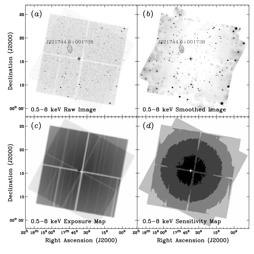
Figure 3: (a) Full-band (0.5–8 keV) raw image of the $\approx$400 ks SSA22 field. This image was constructed following the procedure outlined in $\S$3.1 and has been binned by a factor of four in both right ascension and declination. The location of the exposure-weighted average aim point has been shown with a cross symbol and the extended source J221744.6+001738 ellipse has been outlined (see $\S$5 for discussion). (b) Adaptively-smoothed exposure-corrected full-band image of SSA22. This image was created following the techniques discussed in $\S$3.1. (c) Full-band exposure map of SSA22. The exposure map was created following the procedure outlined in $\S$3.1. The grayscales are linear with the darkest areas corresponding to the highest effective exposure times (with a maximum pixel value of $\approx$388 ks). Note the chip gaps in running between the four ACIS-I CCDs. (d) Full-band sensitivity map of SSA22. This sensitivity map has been created following the procedure outlined in $\S$3.3. The gray-scale levels (running from black to light gray) indicate regions with flux limits (in units of ergs cm^-2 s^-1) of $<2\times 10^{-16}$, 2–5 $\times$ $10^{-16}$, 5–10 $\times$ $10^{-16}$, and $>10^{-15}$, respectively.

3.2 Point-Source Searching and Catalog Production

Our point-source catalog production has been tailored to generate source lists that can be directly comparable with those from previous studies of the CDFs (e.g., Alexander et al. 2003; Lehmer et al. 2005; Luo et al. 2008) to enable comparative studies; however, our procedure and main catalog definitions differ in a number of important ways. The main differences in the catalog production procedure adopted here are as follows:

1.—We first created a candidate-list catalog of sources detected by wavdetect at a liberal false-positive probability threshold of 10^-5. We then created a more conservative main catalog, in which we evaluated the significance of each detected source candidate (see point 2 below) and included only X-ray sources that had high statistical probabilities of being true sources considering their local backgrounds. This approach produced point-source catalogs that are of similar quality to those produced by running wavdetect at the more typical false-positive probability threshold of $10^{-6}$, but allowed for flexibility in the inclusion of additional legitimate sources that fell below the $10^{-6}$ threshold (see $\S$3.2.1 for further details).

2.—While computing X-ray source properties and evaluating the significance of each detected source (i.e., the probability of it being a true source), we made wide use of the ACIS EXTRACT (hereafter, AE) point-source analysis software. AE contains algorithms that allow for appropriate computation of source properties when multiple observations with different roll angles and/or aim points are being combined and analysed (see discussion below for further details). Our adopted procedure has previously been utilised in similar forms by other groups, including, e.g., the X-ray source catalogs produced in the Chandra Orion ultra-deep project (COUP; e.g., Getman et al. 2005) and the AEGIS-X survey (e.g., Nandra et al. 2005; Laird et al. 2009).

3.2.1 Candidate-List Catalog Production

We began by generating a candidate-list catalog of X-ray point sources using the CIAO tool wavdetect (Freeman et al. 2002). We performed our searching in the three standard band (i.e., the FB, SB, and HB) images using a “$\sqrt{2}$ sequence” of wavelet scales (i.e., 1, $\sqrt{2}$, 2, $2\sqrt{2}$, 4, $4\sqrt{2}$, and 8 pixels) and a false-positive probability threshold of $10^{-5}$. We note that the use of a false-positive probability threshold of $10^{-5}$ is expected to generate a non-negligible number of spurious sources with low source counts ($\;\buildrel<\over{\sim}\;$2–3); however, as noted by Alexander et al. (2001), real sources can be missed using a more stringent source-detection threshold (e.g., $10^{-6}$). In $\S$3.2.2 below, we create a main catalog of sources by determining the significance of each source in our candidate-list catalog and excising sources with individual detection significances falling below an adopted threshold.

Figure 4: (a) Total solid angle with at least the vignetting-corrected effective exposure indicated on the abscissa for each of the three standard bands. We find that $\;\buildrel>\over{\sim}\;$60 per cent of the entire $\approx$330 arcmin² field has an effective exposure exceeding 300 ks (vertical long-dashed line). (b) Solid angle versus flux limit for the three standard bands. These curves were computed using the sensitivity maps described in $\S$3.3. In the most sensitive region of the SSA22 field, within the most sensitive 10 arcmin² region (predominantly around the Chandra aim point), the flux limits are $\approx$$1.7\times 10^{-16}$ (full band), $\approx$$5.7\times 10^{-17}$ (soft band), and $\approx$$3.0\times 10^{-16}$ (hard band) ergs cm^-2 s^-1.

Our candidate-list catalog (constructed using a false-positive probability threshold of $10^{-5}$) contained a total of 350 X-ray source candidates. For this candidate list, we required that a point source be detected in at least one of the three standard bands with wavdetect. We utilise full-band source positions for all sources with full band detections; for sources not detected in the full band, we utilised, in order of priority, soft band and hard band source positions. Cross-band matching was performed using a 2.5 arcsec matching radius for sources within 6.0 arcmin of the exposure-weighted mean aim point and 4.0 arcsec for sources at off-axis angles $>$6.0 arcmin. These matching radii were chosen based on inspection of histograms showing the number of matches obtained as a function of angular separation (e.g., see §2 of Boller et al. 1998); with these radii, the mismatch probability is expected to be $\;\buildrel<\over{\sim}\;$1 per cent over the entire field. While matching the three standard band source lists, we found that no source in one band matched to more than one source in another band.

Using AE, we improved the wavdetect source positions using centroiding and matched-filter techniques. The matched-filter technique convolves the full-band image in the vicinity of each source with a combined PSF. The combined PSF is produced by combining the “library” PSF of a source for each relevant observation (from Table 1), weighted by the number of detected counts. This technique takes into account the fact that, due to the complex PSF at large off-axis angles, the X-ray source position is not always located at the peak of the X-ray emission. For sources further than 8 arcmin from the average aim-point, the matched-filter technique provides positions that have median offsets to potential $K$-band counterparts (within a matching radius of 1.5 arcsec) that are $\approx$0.1 arcsec smaller than such offsets found for both centroid and wavdetect source positions. For sources with off-axis angles $\theta$ $<$ 8 arcmin, we found that the centroid positions had the smallest median offsets to $K$-band counterparts compared with matched-filter and wavdetect positions. Thus, for our candidate-list source positions, we utilised centroid positions for $\theta$ $<$ 8 arcmin and matched-filter positions for $\theta$ $\geq$ 8 arcmin. The median source position shift relative to wavdetect source positions was $\approx$0.26 arcsec (quartile range of $\approx$0.1–0.5 arcsec).

For our candidate-list catalog sources, we performed photometry using AE. For each X-ray source in each of the four observations listed in Table 1, AE extracted full band source events and exposure times (using the events lists and exposure maps discussed in $\S$2.2 and $\S$3.1, respectively) from all pixels that had exposure within polygonal regions centred on the X-ray position. Each polygonal region was constructed by tracing the $\approx$90 per cent encircled-energy fraction contours of a local PSF measured at 1.497 keV that was generated using CIAO tool mkpsf. Upon inspection, we found 16 sources (i.e., eight source pairs) had significantly overlapping polygonal extraction regions. For these sources, we utilised smaller extraction regions (ranging from 30–75 per cent encircled energy fractions), which were chosen to be as large as possible without overlapping. For each source, the source events and exposure times from all relevant observations were then summed to give the total source events $S_{\rm src}$ and exposure times $T_{\rm src}$.

For each source in our candidate-list catalog, local full band background events and exposure times were then extracted from each observation. This was achieved by creating full band events lists and exposure maps with all candidate-list catalog sources masked out of circular masking regions of radius $1.1\times$ the size of the $\approx$99.9 per cent encircled energy fraction at 1.497 keV (estimated using each local PSF). The radii of the masked out regions cover a range of $\approx$11.6–17.9 arcsec and have a median value of $\approx$12.8 arcsec. Using these masked data products, AE then extracted events and exposure times from a larger background-extraction circular aperture that was centred on the source. The size of the background extraction radius varied with each source and was chosen to encircle $\approx$170 full-band (resulting in $\approx$40 soft-band and $\approx$130 hard-band) background events for each observation. The background extraction radius is therefore affected by the masking of nearby sources and could potentially become large and non-local for the case of crowded regions. However, our candidate-list catalog has negligible source crowding and therefore the radii of our background extraction regions remain relatively small ($\approx$22–55 arcsec) and are therefore representative of the local backgrounds. For each source, the background events and exposure times from all relevant observations were then summed to give total background events $S_{\rm bkg}$ and exposure times $T_{\rm bkg}$.

The source and local background events extracted above were then filtered by photon energy to produce source and local background counts appropriate for each of the three standard bands. For each bandpass, net source counts $N^{E_{1}-E_{2}}$ (where $E_{1}$ and $E_{2}$ represent the lower and upper energy bounds, respectively, of an arbitrary bandpass) were computed following $N^{E_{1}-E_{2}}=[S_{\rm src}^{E_{1}-E_{2}}-S_{\rm bkg}^{E_{1}-E_{2}}T_{\rm src}/T_{\rm bkg}]/\gamma_{\rm EEF}^{E_{1}-E_{2}}$, where $\gamma_{\rm EEF}^{E_{1}-E_{2}}$ is the encircled-energy fraction appropriate for the source extraction region and bandpass. For the soft and hard bands, $\gamma_{\rm EEF}^{\rm 0.5-2~{}keV}$ and $\gamma_{\rm EEF}^{\rm 2-8~{}keV}$ were approximated using PSF measurements at 1.497 keV and 4.51 keV, respectively. For the full band, we used the approximation $\gamma_{\rm EEF}^{\rm 0.5-8~{}keV}\approx 1/2(\gamma_{\rm EEF}^{\rm 0.5-2~{}keV}+\gamma_{\rm EEF}^{\rm 2-8~{}keV})$. As a result of our liberal searching criteria used for generating the candidate-list catalog, many sources have small numbers of counts. We find that 51 (3) candidate-list catalog sources have $<$5 ($<$0) net counts in all three of the standard bandpasses. In the next section, we evaluate the reliability of the sources detected in our candidate-list catalog on a source-by-source basis to create a more conservative main catalog of reliable sources.

3.2.2 Main Chandra Source Catalog Selection

As discussed above, our candidate-list catalog of 350 X-ray point-sources produced by running wavdetect at a false-positive probability threshold of $10^{-5}$ is expected to have a significant number of false sources. If we conservatively treat our three standard band images as being independent, it appears that $\approx$130 ($\approx$37 per cent) false sources are expected in our candidate-list Chandra source catalog for the case of a uniform backgrounds over $\approx$$1.3\times 10^{7}$ pixels (i.e., all three bands). However, since wavdetect suppresses fluctuations on scales smaller than the PSF, a single pixel usually should not be considered a source detection cell, particularly at large off-axis angles. Hence, our false-source estimates are conservative. As quantified in $\S$3.4.1 of Alexander et al. (2003) and by source-detection simulations (P. E. Freeman 2005, private communication), the number of false-sources is likely $\approx$2–3 times less than our conservative estimate, leaving only $\approx$40–65 false sources; still potentially a significant fraction (i.e., $\;\buildrel<\over{\sim}\;$19 per cent) of our candidate-list list of 350 point sources.

In order to produce a more conservative main catalog of Chandra point-sources and remove likely false sources, we evaluated for each source the binomial probability $P$ that no source exists given the measurements of the source and local background (see $\S$3.2.1 for details on the measurements of source and local background events). The quantity $P$ is computed using AE for each of the three standard bands (see also Appendix A2 of Weisskopf et al. 2007 for further details). For a source to be included in our main catalog, we required $P<0.01$ in at least one of the three standard bands. This criterion gave a total of 297 sources, which make up our main catalog (see $\S$3.2.3 and Table 2 below).

Figure 5: (top) One minus the AE binomial probability that no source exists ($1-P$) versus the logarithm of the minimum wavdetect probability for the 350 sources in our candidate-list catalog (small filled circles; see $\S\S$ 3.2.1 and 3.2.2). We note that for a given value of the wavdetect probability, the majority of the sources have $1-P=1$, causing clumping of the symbols. The dashed horizontal line at $1-P=0.99$ shows the adopted lower threshold used for including a source in our main catalog. (bottom) The percentage of sources in the candidate-list catalog with $1-P>0.99$, which were included in our main catalog, as a function of minimum wavdetect probability (five-pointed stars). The number of sources with $1-P>0.99$ versus the number of candidate-list catalog sources detected at each minimum wavdetect probability has been annotated in the figure. We find that the fraction of candidate-list catalog sources included in our main catalog falls from $\approx$99.5 per cent to $\approx$56.9 per cent between minimum wavedetect probabilities of $10^{-8}$ and $10^{-5}$.

Our adopted binomial probability-based detection criterion has a number of advantages over a direct wavdetect approach including (1) the more detailed treatment of complex source extraction regions for exposures with multiple observations that have different aim points and roll angles, (2) better source position determination before count extraction and probability measurements are made, and (3) a more transparent mathematical criterion (i.e., the binomial probability) that is used for the detection of a source. However, this approach has the disadvantage that we do not approximate the shape of the PSF, as is done by wavdetect through the use of the “Mexican Hat” source detection wavelet. As we will highlight below, our adopted procedure recovers almost all of the sources detected with wavdetect at a false-positive probability threshold of $10^{-6}$ and a large number of additional real sources detected at $10^{-5}$; therefore, this procedure is preferred over a direct wavdetect approach.

To give a more detailed wavdetect perspective on source significance, we ran wavdetect over the three standard band images at additional false-positive probability thresholds of $10^{-6}$, $10^{-7}$, and $10^{-8}$ and found detections for 248 ($\approx$71 per cent), 211 ($\approx$60 per cent), and 190 ($\approx$54 per cent) of the 350 candidate-list catalog sources, respectively. Out of the 53 sources that were excluded from our candidate-list catalog to form our main catalog (297 sources; down from the 350 sources in our candidate-list catalog), 9 had wavdetect false-positive probability detection thresholds $\leq$$10^{-6}$. For convenience, in Appendix A we present the properties of the nine sources with wavdetect detection threshold $\leq$$10^{-6}$ that were not included in the main catalog. This provides the option for the reader to construct a pure wavdetect catalog down to a false-positive probability threshold of $10^{-6}$, $10^{-7}$, or $10^{-8}$, to make it more consistent with previous Chandra source catalogs.

In Figure 5, we present the AE-determined binomial probabilities and the fraction of sources included in the main catalog as a function of the minimum wavdetect probability for the 350 candidate-list catalog sources. Our main catalog includes 58 sources that had minimum wavdetect probabilities of $10^{-5}$. For these 58 sources, we performed cross-band matching between the X-ray source positions and the $K$-band and Spitzer 3.6, 4.5, 5.8, and 8.0$\mu$m IRAC source positions. In total, we find that 33 ($\approx$56.9 per cent) of the 58 sources had at least one infrared counterpart within a 1.5 arcsec matching radius; by comparison, we find that the infrared counterpart fraction for the remaining main Chandra catalog sources (i.e., those with minimum wavdetect probabilities $\leq$$10^{-6}$) is $\approx$89.1 per cent. We estimated the expected number of false matches by shifting the main Chandra catalog source positions by a constant offset (5.0 arcsec) and rematching them to the infrared positions. We performed four such “shift and rematch” trials in unique directions and found that on an average $\approx$8.2${}^{+2.1}_{-1.7}$ per cent of the shifted source positions had an infrared match. We therefore estimate that of the 58 main catalog sources that had minimum wavdetect probabilities of $10^{-5}$, at least $\approx$27–29 ($\approx$46.6–50.4 per cent) have true infrared counterparts that are associated with the X-ray sources; we note that since these are typically fainter X-ray sources we might expect a lower matching fraction than that found for the brighter X-ray sources. This analysis illustrates that our main catalog selection criteria effectively identifies a significant number of additional real X-ray sources below the traditional $10^{-6}$ wavdetect searching threshold through X-ray selection alone.

3.2.3 Properties of Main Catalog Sources

To estimate positional errors for all 297 sources in our main Chandra catalog, we performed cross-band matching between the X-ray and $K$ bands. As discussed in $\S$2.2, the $K$-band sources have highly accurate and precise absolute astrometric positions ($\;\buildrel<\over{\sim}\;$0.1 arcsec positional errors) and reach a 5$\sigma$ limiting magnitude of $K\approx 20.9$ (Vega), a regime where the source density is relatively low ($\approx$80,000 sources deg^-2) and therefore ideal for isolating highly-confident near-infrared counterparts to X-ray sources with little source confusion. Using a matching radius of 2.5 arcsec, we find that 193 ($\approx$65 per cent) X-ray sources have $K$-band counterparts down to $K\approx 20.9$. For 13 of our main catalog sources, there was more than one $K$-band counterpart within 2.5 arcsec. In these cases, we chose the source with the smallest offset as being the most likely counterpart. We computed the expected number of false matches using the shift and rematch technique described in $\S$3.2.2 and estimate that $\approx$26.3 ($\approx$14 per cent) of the matches are false (with a random offset of 1.72 arcsec). We note that our choice to use the large 2.5 arcsec matching radius is based on the fact that the Chandra positional errors are expected to be of this order for low-count sources that are far off-axis where the PSF is large. A more conservative matching criterion is used to determine likely $K$-band counterparts, which are reported in the main catalog (see description of columns [17] and [18] of Table 2 below). In a small number of cases, the X-ray source may be offset from the centroid of the $K$-band source even though both are associated with the same galaxy (e.g., a $z\lower 2.15277pt\hbox{$\;\buildrel<\over{\sim}\;$}0.3$ galaxy with extended $K$-band emission from starlight that also has an off-nuclear ultraluminous X-ray binary with $L_{\rm X}$ $\approx$ 10³⁸–$10^{40}$ ergs s^-1; see e.g., Hornschemeier et al. 2004; Lehmer et al. 2006).

In Figure 6, we show the positional offset between the X-ray and $K$-band sources versus off-axis angle. The median offset is $\approx$0.36 arcsec; however, there are clear off-axis angle and source-count dependencies. The off-axis angle dependence is due to the PSF becoming broad at large off-axis angles, while the count dependency is due to the fact that sources having larger numbers of counts provide a better statistical sampling of the local PSF. To estimate the positional errors of our sources and their dependencies, we implemented the parameterization provided by Kim et al. (2007), derived for sources in the Chandra Multiwavelength Project (ChaMP):

$$\log\Delta_{\rm X}=a_{0}+a_{1}\theta+a_{2}\log C,$$ (1)

where $\Delta_{\rm X}$ is the positional error in arcseconds, $\theta$ is the off-axis angle in units of arcminutes, $C$ is the net counts from the energy band used to determine the position, and $a_{0}$, $a_{1}$, and $a_{2}$ are constants. In equation 1, $a_{0}$ provides a normalization to the positional error and $a_{1}$ and $a_{2}$ indicate the respective off-axis angle and source-count dependencies. Initial values of $a_{0}$, $a_{1}$, and $a_{2}$ were determined by performing multivariate $\chi^{2}$ minimization of equation 1, using our main catalog and the X-ray/$K$-band offsets as a proxy for the positional error. Using the resulting best-fit equation, the value of $a_{0}$ was subsequently adjusted upward by a constant value until $\;\buildrel>\over{\sim}\;$80 per cent of the main catalog sources with $K$-band counterparts had $\Delta_{\rm X}$ values that were larger than their X-ray/$K$-band offsets. This resulted in values of $a_{0}=-0.0402$, $a_{1}=0.0960$, and $a_{2}=-0.3542$; applying these values to equation 1 gives positional errors with $\approx$80 per cent confidence. Note that the values of $a_{1}$ and $a_{2}$ are similar to those found from ChaMP (see equation 12 of Kim et al. 2007); however, due to differences in adopted confidence levels ($\approx$95 per cent for ChaMP) and the positional refinements described in $\S$3.2.1, our value of $a_{0}$ is smaller by $\approx$0.4 dex.

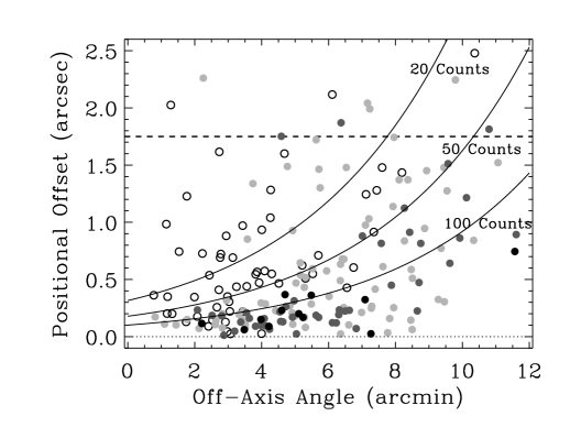
Figure 6: Positional offset versus off-axis angle for sources in the main Chandra catalog that were matched to near-infrared sources from the UKIDSS DXS $K$-band image to within 2.5 arcsec. Symbol grayscales indicate various ranges of net source counts including $<$20 (open circles), 20–50 (light gray), 50–100 (dark gray), and $>$100 (filled black circles) net counts. Our $\approx$80 per cent positional error curves, computed following equation 1, have been indicated for sources with 20, 50, and 100 net counts. For reference, we have highlighted the median offset (1.72 arcsec; horizontal dashed line) found for source matching to random positions; this was obtained using the shift and rematch technique described in $\S$3.2.2.

The main Chandra source catalog is presented in Table 2, and the details of the columns are given below.

Column (1) gives the source number. Sources are listed in order of increasing right ascension. Source positions were determined following the procedure discussed in $\S$3.2.1.

Columns (2) and (3) give the right ascension and declination of the X-ray source, respectively. To avoid truncation error, we quote the positions to higher precision than in the International Astronomical Union (IAU) registered names beginning with the acronym “CXO SSA22” for “Chandra X-ray Observatory Small Selected Area 22.” The IAU names should be truncated after the tenths of seconds in right ascension and after the arcseconds in declination.

Column (4) and (5) give the AE significance, presented as unity minus the computed binomial probability $P$ that no X-ray source exists ($1-P$), and the logarithm of the minimum false-positive probability run with wavdetect in which each source was detected, respectively. Lower values of the binomial probability and false-positive probability threshold indicate a more significant source detection. We find that 189, 20, 30, and 58 sources have minimum wavdetect false-positive probability thresholds of $10^{-8}$, $10^{-7}$, $10^{-6}$, and $10^{-5}$, respectively.

Column (6) gives the $\approx$80 per cent positional uncertainty in arcseconds, computed following equation 1 (see above), which is dependent on the off-axis angle and the net counts of the source in the detection band used to determine the photometric properties (see columns [8]–[16]).

Column (7) gives the off-axis angle for each source in arcminutes. This is calculated using the source position given in columns (2) and (3) and the exposure-weighted mean aim point.

Columns (8)–(16) give the net background-subtracted source counts and the corresponding $1\sigma$ upper and lower statistical errors (from Gehrels 1986), respectively, for the three standard bands. Source counts and statistical errors have been calculated by AE using the position given in columns (2) and (3) for all bands and following the methods discussed in detail in $\S$3.2.1, and have not been corrected for vignetting. We note that the extraction of source counts and the computation of statistical errors was performed for all sources in our candidate-list catalog of sources detected using wavdetect at a false-positive probability threshold of $1\times 10^{-5}$. Since all candidate-list catalog sources were masked when calculating local backgrounds for our main catalog sources (see $\S$3.2.1), this could in principle have a mild effect on background calculations in cases where lower-significance candidate-list catalog sources (i.e., sources that would later not be included in the main catalog) were near main catalog sources. We note, however, that since the number of candidate-list catalog sources that were excluded from our main catalog is small (i.e., 53 sources), there is little overlap between these sources and the background extraction regions of our main catalog. We found that 43 ($\approx$14 per cent) of the 297 main catalog background extraction regions had some overlap with the $\approx$90 per cent PSF regions of at least one of the 53 excluded candidate-list catalog sources. Since the 53 excluded candidate-list catalog sources already have count estimates that were consistent with the local background, we conclude that this will not have a significant effect on our main catalog source properties.

To be consistent with our point-source detection criteria defined in $\S$3.2.2, we considered a source to be “detected” for photometry purposes in a given band if the AE-computed binomial probability for that band has a value of $P<0.01$. When a source is not detected in a given band, an upper limit is calculated; these sources are indicated as a “$-$1” in the error columns. All upper limits were computed using the AE-extracted photometry (see $\S$3.2.1) and correspond to the 3$\sigma$ level appropriate for Poisson statistics (Gehrels 1986).

Table 2: Main Chandra Catalog

	X-ray Coordinates		Detection Probability				Net Counts
Source					Pos. Error	$\theta$
Number	$\alpha_{\rm J2000}$	$\delta_{\rm J2000}$	AE	wavdetect	(arcsec)	(arcmin)	0.5–8 keV	0.5–2 keV	2–8 keV
(1)	(2)	(3)	(4)	(5)	(6)	(7)	(8)–(10)	(11)–(13)	(14)–(16)
1	22 16 51.96	+00 18 49.0	1.000	$-$8	3.60	11.77	32.1${}^{+10.0}_{-8.8}$	16.5${}^{+6.4}_{-5.2}$	15.6${}^{+8.4}_{-7.2}$
2	22 16 55.25	+00 21 54.2	1.000	$-$8	3.37	12.22	51.1${}^{+12.7}_{-11.5}$	32.8${}^{+8.5}_{-7.3}$	$<$30.3
3	22 16 56.32	+00 16 57.7	1.000	$-$8	2.27	10.34	48.0${}^{+10.6}_{-9.4}$	39.1${}^{+8.3}_{-7.0}$	$<$22.1
4	22 16 58.20	+00 21 58.6	1.000	$-$8	1.35	11.61	458.8${}^{+28.2}_{-27.0}$	249.7${}^{+19.2}_{-18.1}$	208.5${}^{+21.3}_{-20.1}$
5	22 16 58.19	+00 18 55.1	1.000	$-$8	2.21	10.22	48.3${}^{+16.0}_{-14.8}$	19.0${}^{+8.7}_{-7.5}$	29.5${}^{+14.1}_{-12.9}$
6	22 16 59.08	+00 15 13.4	1.000	$-$8	1.44	9.57	107.1${}^{+13.4}_{-12.2}$	75.6${}^{+10.7}_{-9.5}$	30.6${}^{+8.9}_{-7.6}$
7	22 17 00.33	+00 19 55.2	1.000	$-$8	1.30	10.12	201.9${}^{+21.0}_{-19.9}$	127.0${}^{+14.4}_{-13.2}$	73.9${}^{+16.1}_{-14.8}$
8	22 17 00.50	+00 21 23.7	1.000	$-$8	1.43	10.80	236.1${}^{+21.8}_{-20.6}$	158.5${}^{+15.7}_{-14.5}$	76.2${}^{+15.9}_{-14.6}$
9	22 17 02.23	+00 13 09.5	0.994	$-$7	2.08	9.00	26.8${}^{+13.3}_{-12.1}$	$<$19.5	26.0${}^{+12.2}_{-11.0}$
10	22 17 03.00	+00 15 25.7	0.997	$-$5	1.76	8.47	30.7${}^{+13.0}_{-11.8}$	$<$21.5	$<$34.5
11	22 17 04.90	+00 09 39.3	1.000	$-$8	1.06	9.92	315.8${}^{+23.6}_{-22.4}$	145.0${}^{+15.0}_{-13.8}$	171.3${}^{+18.9}_{-17.7}$
12	22 17 05.41	+00 15 14.0	1.000	$-$8	0.67	7.88	320.7${}^{+21.8}_{-20.6}$	208.6${}^{+16.9}_{-15.7}$	110.0${}^{+14.4}_{-13.2}$
13	22 17 05.63	+00 19 46.3	1.000	$-$6	1.80	8.87	37.2${}^{+12.4}_{-11.2}$	$<$17.8	35.3${}^{+11.5}_{-10.3}$
14	22 17 05.82	+00 22 27.7	0.993	$-$5	3.68	10.37	$<$46.3	12.6${}^{+11.1}_{-7.0}$	$<$39.7
15	22 17 05.83	+00 22 24.7	0.998	$-$7	2.74	10.34	28.2${}^{+16.4}_{-12.4}$	$<$32.2	$<$44.7
16	22 17 06.14	+00 13 38.0	1.000	$-$8	1.12	7.93	79.4${}^{+13.6}_{-12.4}$	39.0${}^{+8.9}_{-7.6}$	40.4${}^{+11.1}_{-9.9}$
17	22 17 06.69	+00 18 38.5	1.000	$-$6	1.71	8.15	27.3${}^{+10.7}_{-9.5}$	19.7${}^{+7.2}_{-6.0}$	$<$25.9
18	22 17 07.04	+00 14 29.8	0.997	$-$5	1.63	7.53	21.4${}^{+9.9}_{-8.7}$	$<$17.3	$<$26.4
19	22 17 07.73	+00 19 58.3	1.000	$-$8	1.56	8.51	44.6${}^{+12.4}_{-11.2}$	$<$17.0	42.2${}^{+11.7}_{-10.4}$
20	22 17 09.60	+00 18 00.1	1.000	$-$8	1.33	7.24	31.7${}^{+10.2}_{-9.0}$	24.1${}^{+7.3}_{-6.1}$	$<$23.4
21	22 17 09.82	+00 08 56.1	1.000	$-$8	1.45	9.46	99.4${}^{+15.6}_{-14.4}$	56.0${}^{+10.3}_{-9.1}$	43.2${}^{+12.4}_{-11.2}$
22	22 17 10.04	+00 13 03.5	1.000	$-$8	1.04	7.16	59.9${}^{+11.7}_{-10.5}$	42.9${}^{+8.9}_{-7.7}$	16.4${}^{+8.4}_{-7.2}$
23	22 17 10.10	+00 11 59.7	1.000	$-$8	0.80	7.57	162.9${}^{+16.4}_{-15.3}$	110.8${}^{+12.8}_{-11.6}$	50.8${}^{+11.1}_{-9.8}$
24	22 17 10.42	+00 06 03.9	1.000	$-$8	1.16	11.57	684.0${}^{+32.0}_{-30.9}$	424.1${}^{+23.7}_{-22.6}$	257.3${}^{+22.2}_{-21.0}$
25	22 17 10.60	+00 11 05.1	1.000	$-$8	1.43	7.96	39.9${}^{+11.7}_{-10.5}$	27.7${}^{+7.8}_{-6.6}$	$<$28.1
26	22 17 10.77	+00 17 16.7	0.999	$-$7	1.50	6.75	16.4${}^{+8.2}_{-7.0}$	$<$12.2	17.0${}^{+7.8}_{-6.5}$
27	22 17 11.13	+00 19 11.9	1.000	$-$8	1.18	7.39	48.6${}^{+11.2}_{-10.0}$	35.2${}^{+8.2}_{-7.0}$	$<$24.9
28	22 17 11.26	+00 19 54.6	1.000	$-$8	0.98	7.74	102.8${}^{+14.1}_{-12.9}$	63.2${}^{+10.3}_{-9.1}$	39.1${}^{+10.5}_{-9.2}$
29	22 17 11.94	+00 17 05.2	1.000	$-$8	1.09	6.41	33.1${}^{+9.3}_{-8.0}$	15.7${}^{+6.1}_{-4.8}$	17.4${}^{+7.7}_{-6.4}$
30	22 17 12.04	+00 12 44.1	1.000	$-$8	0.51	6.83	374.5${}^{+22.7}_{-21.5}$	33.9${}^{+8.0}_{-6.8}$	347.7${}^{+22.0}_{-20.8}$

NOTE. — Table 2 is presented in its entirety in the electronic version; an abbreviated version of the table is shown here for guidance as to its form and content. The full table contains 44 columns of information for all 297 Chandra sources. Meanings and units for all columns have been summarized in detail in $\S$ 3.2.3.

Columns (17) and (18) give the right ascension and declination of the near-infrared source centroid, which was obtained by matching our X-ray source positions (columns [2] and [3]) to DXS UKIDSS $K$-band positions using a matching radius of 1.5 times the positional uncertainty quoted in column (6). For five X-ray sources more than one near-infrared match was found, and for these sources the source with the smallest offset was selected as the most probable counterpart. Using these criteria, 183 ($\approx$63 per cent) of the sources have $K$-band counterparts. Note that the matching criterion used here is more conservative than that used in the derivation of our positional errors discussed above (i.e., the median value of 1.5 times the positional uncertainty is $\approx$1.3 arcsec). Sources with no optical counterparts have right ascension and declination values set to “00 00 00.00” and “+00 00 00.0”.

Column (19) indicates the measured offset between the $K$-band and X-ray source positions in arcseconds. Sources with no $K$-band counterparts have a value set to “$-$1.” We find a median offset of 0.35 arcsec.

Column (20) provides the corresponding $K$-band magnitude (Vega) for the source located at the position indicated in columns (17) and (18). Sources with no $K$-band counterpart have a value set to “$-$1.”

Table 3: Summary of Chandra Source Detections

		Detected Counts Per Source				Flux Per Source
Band	Number of
(keV)	Sources	Maximum	Minimum	Median	Mean	Maximuma	Minimuma	Mediana	Meana
Full (0.5–8) …………	278	1965.4	4.8	33.5	105.4	$-$13.2	$-$15.8	$-$14.7	$-$14.3
Soft (0.5–2) …………	248	1228.9	3.0	18.2	68.5	$-$13.7	$-$16.3	$-$15.4	$-$14.9
Hard (2–8) …………	206	746.7	4.0	26.0	57.0	$-$13.4	$-$15.6	$-$14.7	$-$14.4

^aValues in these columns represent the logarithm of the maximum, minimum, median, and mean fluxes in units of ergs cm^-2 s^-1.

Columns (21)–(25) give the AB magnitudes for the Subaru $B$, $V$, $R$, $i^{\prime}$, and $z^{\prime}$ optical bands, respectively. Information regarding the Subaru observations can be found in $\S$2 of Hayashino et al. (2004). The Subaru observations cover the entire Chandra observed region of SSA22 and reach 5$\sigma$ limiting depths of $B=26.5$, $V=26.6$, $R=26.7$, $i^{\prime}=26.4$, and $z^{\prime}=25.7$ AB magnitudes. Using a constant 1.5 arcsec matching radius, we found that 175, 202, 211, 210, and 205 of the main catalog sources had $B$, $V$, $R$, $i^{\prime}$, and $z^{\prime}$ band counterparts, respectively; 213 of the main catalog sources had at least one optical counterpart. Based on the shift and rematch technique described in $\S$3.2.2, we estimate that $\approx$45.8${}^{+6.9}_{-6.7}$ are expected to be false matches. When a counterpart is not identified for a given IRAC band, a value of “$-$1” is listed for that band.

Columns (26)–(29) give the AB magnitudes for the Spitzer IRAC bands at 3.6, 4.5, 5.8, and 8.0$\mu$m, respectively. Information regarding the IRAC observations can be found in $\S$2.1 of Webb et al. (2009). The IRAC observations cover the majority of the Chandra observed region of SSA22 and reach 5$\sigma$ limiting depths of 23.6, 23.4, 21.6, and 21.5 AB magnitudes for the 3.6, 4.5, 5.8, and 8.0$\mu$m bands, respectively. Using a constant 1.5 arcsec matching radius, we found that 212, 217, 173, and 174 of the main catalog sources had 3.6, 4.5, 5.8, and 8.0$\mu$m counterparts, respectively; 234 of the main catalog sources have at least one IRAC counterpart. Based on the shift and rematch technique described in $\S$3.2.2, we estimate that $\approx$21.3${}^{+5.7}_{-4.6}$ are expected to be false matches. When a counterpart is not identified for a given IRAC band, a value of “$-$1” is listed for that band. We note that a small area of the Chandra exposure has no overlapping IRAC observations (see Fig. 2), and sources in these regions have a value of “$-$2” listed in these columns.

Column (30) provides the best available optical spectroscopic redshift for each X-ray source when the optical and X-ray positions were offset by less than 1.5 arcsec. Spectroscopic redshifts for 46 sources are provided: 31 sources from the Garilli et al. (2008) catalog of the VIMOS VLT Deep Survey (VVDS; Le Fèvre et al. 2005), two sources from the Steidel et al. (2003) LBG survey, four sources from the Matsuda et al. (2005) LAE survey, and nine sources from a new spectroscopic campaign of Chapman et al. (2009, in-preparation). In total, nine of the sources had spectroscopic redshifts within $z=$ 3.06–3.12 ($\Delta v\approx$ 4,000 km s^-1), suggesting that they are likely members of the SSA22 protocluster (see $\S$4 for further details). Sources with no spectroscopic redshift available have a value set to “$-$1.”

Column (31) indicates which optical spectroscopic survey provided the redshift value quoted in column (30). Source redshifts provided by Garilli et al. (2008), Steidel et al. (2003), Matsuda et al. (2005), and Chapman et al. (2009, in-preparation) are denoted with the integer values 1–4, respectively. Sources with no spectroscopic redshift available have a value set to “$-$1.”

Figure 7: (a) The distributions of detected source counts for sources in the main Chandra catalog in the full (top), soft (middle), and hard (bottom) bands. Sources with upper limits have not been included in this plot. The vertical dotted lines indicate the median number of detected counts: 32.7, 18.2, and 25.0 for the full, soft, and hard bands, respectively. Regions where basic ($\approx$100–1000 counts) and detailed ($\;\buildrel>\over{\sim}\;$1,000 counts) X-ray spectroscopic fitting is possible are indicated. The numbers of sources rise toward lower counts before peaking around $\approx$10–30 counts, where our survey is thought to be highly complete. (b) Histograms showing the distributions of X-ray fluxes for sources in the main Chandra catalog in the full (top), soft (middle), and hard (bottom) bands. Sources with upper limits have not been included in this plot. The vertical dotted lines indicate the median fluxes of 15.8, 4.0, and 20.0 $\times$ 10^-16 ergs cm^-2 s^-1 for the full, soft, and hard bands, respectively.

Columns (32)–(34) give the effective exposure times derived from the standard-band exposure maps (see §3.1 for details on the exposure maps). Dividing the counts listed in columns (8)–(16) by the corresponding effective exposures will provide vignetting-corrected and quantum efficiency degradation-corrected count rates.

Columns (35)–(37) give the band ratio, defined as the ratio of counts between the hard and soft bands, and the corresponding upper and lower errors, respectively. Quoted band ratios have been corrected for differential vignetting between the hard band and soft band using the appropriate exposure maps. Errors for this quantity are calculated following the numerical error propagation method described in §1.7.3 of Lyons (1991); this avoids the failure of the standard approximate variance formula when the number of counts is small (see §2.4.5 of Eadie et al. 1971) and has an error distribution that is non-Gaussian. Upper limits are calculated for sources detected in the soft band but not the hard band and lower limits are calculated for sources detected in the hard band but not the soft band. For these sources, the upper and lower errors are set to the computed band ratio. Sources detected only in the full band have band ratios and corresponding errors set to “$-1$.”

Columns (38)–(40) give the effective photon index ($\Gamma_{\rm eff}$) with upper and lower errors, respectively, for a power-law model with the Galactic column density. The effective photon index has been calculated based on the band ratio in column (35).

For sources that are not detected (as per the definition discussed above in the description of columns [8]–[16]) in the hard band or soft band, then lower or upper limits, respectively, are placed on $\Gamma_{\rm eff}$; in these cases, the upper and lower errors are set to the limit that is provided in column (38). When a source is only detected in the full band, then the effective photon index and upper and lower limits are set to 1.4, a value that is representative for faint sources that should give reasonable fluxes.

Columns (41)–(43) give observed-frame fluxes in the three standard bands; quoted fluxes are in units of ergs cm^-2 s^-1. Fluxes have been computed using the counts in columns (8), (11), and (14), the appropriate exposure maps (columns [32]–[34]), and the spectral slopes given in column (38). Negative flux values indicate upper limits. The fluxes have been corrected for absorption by the Galaxy but have not been corrected for material intrinsic to the source. For a power-law model with $\Gamma=1.4$, the soft-band and hard-band Galactic absorption corrections are $\approx$12.6 per cent and $\approx$0.4 per cent, respectively. We note that, due to the Eddington bias, sources with a low number of net counts ($\;\buildrel<\over{\sim}\;$10 counts) may have true fluxes lower than those computed using the basic method used here (see, e.g., Vikhlinin et al. 1995; Georgakakis et al. 2008). However, we aim to provide only observed fluxes here and do not make corrections for the Eddington bias. More accurate fluxes for these sources would require (1) the use of a number-count distribution prior to estimate the flux probabilities for sources near the sensitivity limit and (2) the direct fitting of the X-ray spectra for each observation; these analyses are beyond the scope of the present paper.

Column (44) gives notes on the sources. “O” refers to objects that have large cross-band (i.e., between the three standard bands) positional offsets ($>2$ arcsec); all of these sources lie at off-axis angles $>$5.5 arcmin. “S” refers to close-double or close-triple sources where manual separation was required (see discussion in $\S$3.2.1). “D” refers to a source having an obvious diffraction spike in the $K$-band image, suggesting the source is likely a Galactic star. “LBG” and “LAE” indicate sources included in the Steidel et al. (2003) LBG survey and the Hayashino et al. (2004) LAE survey, respectively. “LAB” indicates that the source was coincident with a LAB in the Geach et al. (2009) study.

Table 4: Sources Detected in One Band but not Another

	Nondetected Energy Band
Detection Band
(keV)	Full	Soft	Hard
Full Band (0.5–8) ……………	…	46	75
Soft Band (0.5–2) ……………	16	…	82
Hard Band (2–8) ………………	3	40	…

NOTE. — For example, of the 278 full band detected sources, there were 46 sources detected in the full band that were not detected in the soft band.

Table 5: Background Parameters

	Mean Background
Bandpass			Total Backgroundc	Count Ratiod
(keV)	(counts pixel-1)a	(counts pixel-1 Ms-1)b	($10^{5}$ counts)	(background/source)
Full Band (0.5–8) …………………	0.072	0.267	3.6	12.1
Soft Band (0.5–2) …………………	0.017	0.065	0.9	5.0
Hard Band (2–8) ……………………	0.055	0.191	2.7	23.0

^aThe mean numbers of background counts per pixel. These are measured from the background images described in $\S$ 3.3.

^bThe mean numbers of counts per pixel divided by the mean effective exposure. These are measured from the exposure maps and background images described in $\S$ 3.3.

^cTotal number of background counts in units of $10^{5}$ counts.

^dRatio of the total number of background counts to the total number of net source counts.

In Table 3 we summarise the source detections, counts, and fluxes for the three standard bands for the main Chandra catalog. In total 297 point sources are detected (i.e., with AE-computed binomial probabilities of $P<0.01$) in one or more of the three standard bands with 278, 248, and 206 sources detected in the full, soft, and hard bands, respectively. In Table 4 we summarise the number of sources detected in one band but not another. All but three of the sources are detected in either the soft or full bands, which is similar to that found for the $\approx$2 Ms CDF-N (one source) and $\approx$2 Ms CDF-S (three sources). From Tables 3 and 4, we find that the fraction of hard-band sources not detected in the soft band is $40/206\approx 19$ per cent, similar to that found in the $\approx$250 ks E-CDF-S, yet somewhat larger than that found in the $\approx$2 Ms CDF-N and $\approx$2 Ms CDF-S, where the fraction is $\approx$14 per cent. In Figure 7$a$, we show the distributions of detected counts in the three standard bands. There are 60 sources with $>$100 full-band counts, for which spectral analyses are possible; there are four sources with $>$1000 full-band counts. We note that the number of sources continuously rises with decreasing detected counts before peaking around the completeness limit of our survey, which occurs at $\approx$10–30 counts depending on the bandpass. In Figure 7$b$ we show the distributions of X-ray flux in the three standard bands. The X-ray fluxes in this survey span roughly three orders of magnitude and have median fluxes of 15.8, 4.0, and $20.0\times 10^{-16}$ ergs cm^-2 s^-1 in the full, soft, and hard bands, respectively.

3.3 Background and Sensitivity Analysis

The faintest sources in our main catalog have $\approx$3 counts (see Table 3). Assuming a $\Gamma=$ 1.4 power law X-ray spectrum with Galactic absorption as given in $\S$1, the corresponding soft-band and hard-band fluxes at the aim points are $\approx$5.0 $\times$ $10^{-17}$ ergs cm^-2 s^-1 and $\approx$2.4 $\times$ $10^{-16}$ ergs cm^-2 s^-1, respectively. This gives a measure of the ultimate sensitivity of the SSA22 survey; however, these values are only relevant for a small region near the aim point and are also subject to significant incompleteness due to Poisson fluctuations of source and background counts at these levels. To determine the sensitivity as a function of position within the SSA22 field, it is necessary to account for the broadening of the PSF with off-axis angle and changes in the effective exposure (due to, e.g., vignetting and chip gaps; see Fig. 3$c$) and background rate across the field. We estimated the sensitivity across the field by calibrating the relationship between the total number of extracted source counts $S$ versus the local background counts $B$ for sources detected in our main catalog. This was achieved mathematically through the use of a binomial probability model, which estimates the value of $S$ given $B$ background counts when a binomial probability of $P=0.01$ is required for a detection. Our resulting relation is

$$\log(S)~{}=\alpha+\beta\log(B)+\gamma[\log(B)]^{2}+\delta[\log(B)]^{3}$$ (2)

where $\alpha=0.6832$, $\beta=0.4956$, $\gamma=0.1124$, and $\delta=0.0003$ are fitting constants. We note that this equation has the same functional form as that used by Lehmer et al. (2005) and Luo et al. (2008), which is appropriate for sources detected using wavdetect at a false-positive probability threshold of $10^{-6}$. However, the constant values differ mildly (most notably in the value of $\alpha$) from those used by Lehmer et al. (2005) and Luo et al. (2008), due to the different detection criteria adopted in this paper. In equation 2, the only component that we need to measure is the local background $B$. To be consistent with our adopted detection criteria described in $\S\S$ 3.2.1 and 3.2.2, we measured the local background in a source cell using the background maps described below assuming an aperture size of 90 per cent of the encircled-energy fraction of the PSF; for ease of computation we utilised circular extraction apertures when measuring local backgrounds (see footnote 2 for circular approximations to the 90 per cent encircled energy fraction). The total background includes contributions from the unresolved cosmic X-ray background, particle background, and instrumental background (e.g., Markevitch 2001; Markevitch et al. 2003; Worsley et al. 2005; Hickox & Markevitch 2006), and for our analyses, we are interested in the total background and therefore do not distinguish between these different components.

We created background maps for all of the three standard-band images by first masking out point sources from our main catalog using circular apertures with radii of $1.1\times$ the $\approx$99.9 per cent PSF encircled-energy fraction radii as defined in $\S$3.2.1. As a result of this masking procedure, the background maps include minimal contributions from main catalog point sources. They will, however, include X-ray counts from the extended sources (e.g., the source J221744.6+001738 described in $\S$5 below), which will cause a mild overestimation of the measured background near and within this source. Extensive testing of the background count distributions in all three standard bandpasses has shown that the X-ray background is nearly Poissonian (see $\S$4.2 of Alexander et al. 2003). We therefore filled in the masked regions for each source with local background counts that were estimated using the probability distribution of counts within an annulus with an inner radius equal to that of the masked out region (i.e., the $1.1\times$ the $\approx$99.9 per cent PSF encircled-energy fraction radius) and an outer radius equal to the size of the background extraction radius defined in $\S$3.2.1; here, the outer radii have sizes in the range of $\approx$1.5–3.7 times the inner radii. The background properties are provided in Table 5. The majority of the pixels have no background counts (e.g., in the full band $\approx$93 per cent of the pixels are zero) and the mean background count rates for these observations are broadly consistent with those presented in Alexander et al. (2003) and Luo et al. (2008).

Following equation 2, we created sensitivity maps using the background and exposure maps. We assumed a $\Gamma=$ 1.4 power-law X-ray spectral energy distribution with Galactic absorption. In Figure 3$d$ we show the full-band sensitivity map, and in Figure 4$b$ we plot the flux limit versus solid angle for the full, soft, and hard bands. We note that the most sensitive $\approx$10 arcmin² region near the aim point has average 0.5–2 keV and 2–8 keV sensitivity limits of $\approx$$5.7\times 10^{-17}$ ergs cm^-2 s^-1 and $\approx$$3.0\times 10^{-16}$ ergs cm^-2 s^-1, respectively.

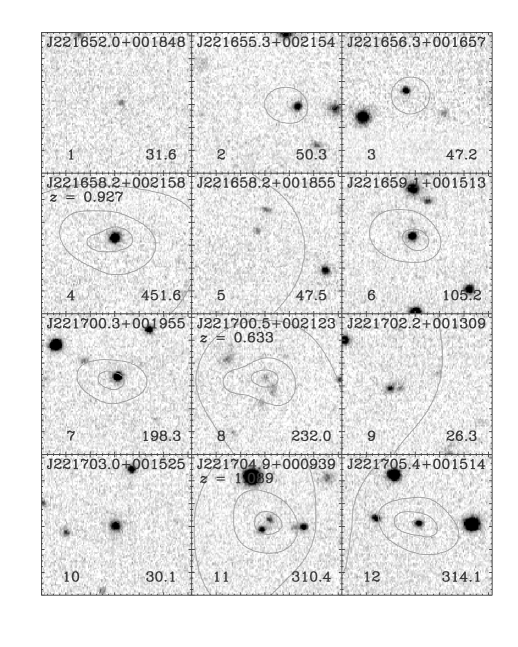
Figure 8: DXS $K$-band postage-stamp images for the sources in the main Chandra catalog with adaptively smoothed X-ray contours overlaid. The contours are logarithmic in scale and range from $\approx$0.00032–32 per cent (with seven total logarithmic scales) of the maximum pixel value in the whole $\approx$330 arcmin² image. The source name, composed of the sexagesimal J2000 source coordinates, has been labelled at the top of each image. The source number (column [1] of Table 2) and full-band net source counts (column [8] of Table 2) have been provided in the lower-left and lower-right corners, respectively; when available, the value of the spectroscopic redshift has been indicated below the source name. Each image is $\approx$24.6 arcsec on a side, and the source of interest is always located at the centre of the image. In several cases no X-ray contours are present, either because these sources were not detected in the full band or the full-band counts are low and CSMOOTH has suppressed the observable emission in the adaptively smoothed image. Only one of the 24 pages of cutouts is included here; all 24 pages are available at the SSA22 website.

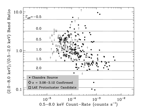
Figure 9: Hard-band–to–soft-band count-rate ratio (i.e., $\Phi_{\rm 2-8~{}keV}/\Phi_{\rm 0.5-2~{}keV}$, where $\Phi$ is the count-rate in units of counts s^-1) versus full-band count-rate for sources in the main Chandra catalog. We note that sources that were only detected in the full-band cannot be plotted in this figure as their band ratios are unconstrained. Horizontal dotted lines show the band ratios corresponding to given effective photon indices; these were calculated using PIMMS. Sources that have been spectroscopically confirmed to lie in the SSA22 protocluster ($z=$ 3.06–3.12) have been indicated with open diamonds and additional LAEs that are likely members of the protocluster are shown with open squares. We note that one of the protocluster sources has not been plotted here, since it was only detected in the full band.

4 Multiwavelength Properties of Main Catalog Sources

In this section, we utilise the multiwavelength data in SSA22 to explore the range of source types detected in our main Chandra catalog and highlight the basic properties of the sources in the protocluster at $z=3.09$. In Figure 8 we show “postage-stamp” images from the DXS $K$-band image with adaptively-smoothed full band contours overlaid for sources included in the main Chandra catalog. The wide range of X-ray source sizes observed in these images is largely due to PSF broadening with off-axis angle. The postage-stamp images show a wide variety of $K$-band source types including unresolved point sources, bright Galactic (Milky Way) stars, extended galaxies, and sources without any obvious counterpart (see column [44] in Table 2).

In Figure 9 we show the band ratio as a function of full-band count rate for sources in the main Chandra catalog. This plot shows that the mean band ratio for sources detected in both the soft and hard bands hardens for fainter fluxes, a trend also observed in the CDFs (e.g., Alexander et al. 2003; Lehmer et al. 2005; Tozzi et al. 2006; Luo et al. 2008). This trend is due to the detection of more absorbed AGNs at low flux levels, and it has been shown that AGNs will continue to dominate the number counts down to 0.5–2 keV fluxes of $\approx$(2–6) $\times$ 10^-18 ergs cm^-2 s^-1 (e.g., Bauer et al. 2004; Kim et al. 2006); however, we expect that an important minority of the sources detected near the flux limit ($\;\buildrel<\over{\sim}\;$$3\times 10^{-16}$ ergs cm^-2 s^-1 in the 0.5–2 keV band) are normal galaxies (e.g., Lehmer et al. 2007, 2008; Ptak et al. 2007). As mentioned above, nine sources in our main catalog have spectroscopic redshifts of $z=$ 3.06–3.12, suggesting that they are members of the SSA22 protocluster. If we include LAEs selected to lie at $z\approx 3.1$ as being likely protocluster members, then we have a total of 12 X-ray detected protocluster sources. From Figure 9, we see that these protocluster sources occupy a range of band-ratios and full band count rates similar to all main catalog sources and do not appear to reside in any unique region of parameter space.

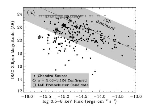
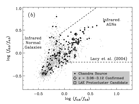
Figure 10: (a) Apparent IRAC 3.6$\mu$m magnitude (AB) versus the logarithm of the 0.5–8 keV flux for sources in the main Chandra catalog. In total 212 sources ($\approx$71 per cent) have 3.6$\mu$m counterparts down to a limiting magnitude of $\approx$23.5 mag. The dashed line and shaded envelope and represents the region where AGN activity is expected to dominate both the 3.6$\mu$m and X-ray emission (see discussion in $\S$4 for details). The majority of our sources have 3.6$\mu$m and full band fluxes that place them in the shaded region, indicating that many of these sources are likely to be AGNs. A significant minority of sources below full band fluxes of $\approx$$3\times 10^{-15}$ ergs cm^-2 s^-1 have relatively low 3.6$\mu$m to X-ray flux ratios. These sources are likely to be a mixture of obscured or low-luminosity AGNs, normal/starburst galaxies, and Galactic stars. (b) Logarithm of the 8.0$\mu$m to 4.5$\mu$m flux density ratio versus the logarithm of the 5.8$\mu$m to 3.6$\mu$m flux density ratio for sources in the SSA22 field that are detected in all four IRAC bands. We have shown all SSA22 sources from the full IRAC catalog (small gray circles) and all Chandra detected sources with IRAC counterparts (black circles). The Lacy et al. (2004) colour-criterion region used to identify AGN candidates has been highlighted with a dashed line boundary.

Figure 10$a$ shows the IRAC 3.6$\mu$m magnitude (AB) versus the full-band flux for sources included in the main catalog. The approximate X-ray to 3.6$\mu$m flux ratio range expected for AGN-dominated systems is indicated. This “AGN region” was calibrated using the 28 X-ray-detected broad-line quasars studied by Richards et al. (2006) and represents the mean logarithm of the 3.6$\mu$m to X-ray flux ration and its 3$\sigma$ scatter. We note that this categorization is only appropriate for powerful AGNs where both X-ray and infrared emission is likely to be dominated by the AGN component (i.e., with little fractional contribution from galactic emission). Therefore, heavily obscured or low-luminosity AGNs that are faint in the X-ray band, but bright in the infrared, can be pushed out of the marked AGN region and into the realm where normal/starburst galaxies and Galactic stars are expected to be found. We find that the majority of our sources lie in the designated AGN region; however, a significant minority of the sources appear to have small X-ray to 3.6$\mu$m flux ratios; these sources are either obscured or low-luminosity AGNs, normal/starburst galaxies, or Galactic stars. The majority of the confirmed protocluster sources are found in the AGN region of Figure 10$a$ (i.e., the shaded region) with the exception of J221742.0+001913, which is X-ray faint but has IRAC colours (see, e.g., Lacy et al. 2004 and Fig. 10$b$) characteristic of AGNs, and it is therefore likely to be powered by a heavily-obscured AGN.

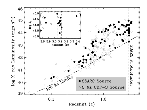
Figure 11: Logarithm of the observed-frame 0.5–8 keV luminosity (i.e., the rest-frame [0.5–8 keV] $\times$ [$1+z$] band) versus redshift for sources in our sample that have optical spectroscopic redshifts (see column [30] of Table 2). The dotted curve shows the average luminosity limit at 5 arcmin off-axis. This limit was determined using the 0.5–8 keV sensitivity map (see $\S$3.3) and our adopted cosmology (see $\S$1). For comparison, we have plotted the sources from the $\approx$2 Ms CDF-S (open circles; Luo et al. 2008). The vertical dashed line highlights the location of the SSA22 protocluster at $z=3.09$, and in the inset plot, we show the region of the plot around the protocluster. This shows the relatively large number of protocluster sources compared to what is found in a low density field like the CDF-S. There are two CDF-S sources within the redshift boundaries of the protocluster; however, only one can be seen due to the large number of SSA22 protocluster sources in this parameter space.

In Figure 10$b$, we show the 8.0$\mu$m to 4.5$\mu$m versus 5.8$\mu$m to 3.6$\mu$m IRAC flux density ratios for sources in the SSA22 IRAC catalogs that are detected in all four IRAC bandpasses (see columns [26]–[29] in Table 2). The AGN region of this diagram, as defined by Lacy et al. (2004), has been outlined with dashed lines. Of the 147 main catalog sources detected in all four IRAC bands, we find that 81 ($\approx$55 per cent) of them lie in the AGN region in Figure 10$b$, as compared with $\approx$25 per cent of all sources in the full IRAC catalog. This result is consistent with the fact that the majority of the X-ray detected sources are likely AGNs. It is of interest to note that a significant number (66; $\approx$45 per cent) of the X-ray-detected sources are not classified as AGNs by the infrared data. While some of these X-ray sources are likely to be normal/starburst galaxies and Galactic stars at least 15 ($\approx$23 per cent) have X-ray properties characteristic of obscured AGNs (i.e., $\Gamma_{\rm eff}\lower 2.15277pt\hbox{$\;\buildrel<\over{\sim}\;$}1$; see, e.g., Donley et al. 2008 for a more detailed study of similar source types in the CDF-S). We note that all of the six protocluster sources (i.e., those with spectroscopic redshifts $z=$ 3.06–3.12 or LAEs) with detections in all four IRAC bands lie in the AGN region in Figure 10$b$.

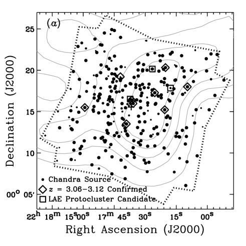
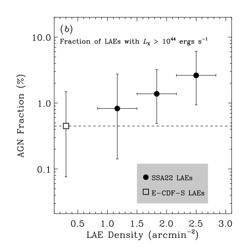
Figure 12: (a) Positions of main Chandra catalog sources. The dotted polygonal and gray contours indicate the Chandra observed region and $z\approx 3.1$ LAE source density levels, respectively (as per Fig. 2). All X-ray–detected sources have been indicated with small filled circles with symbol sizes dependent on AE detection significance, such that more significant sources have larger circles; the largest symbols represent sources with $P<10^{-5}$. We find that the majority of the X-ray detected protocluster sources lie in the highest LAE density regions. (b) Fraction of $z\approx 3$ LAEs hosting an AGN with rest-frame 8–32 keV luminosity larger than $10^{44}$ ergs s^-1 (filled circles) as a function of local LAE density. The field-averaged AGN fraction for $z\approx 3$ LAEs in the E-CDF-S (from Gronwall et al. 2007) has been indicated with an open square and a dashed horizontal line for guidance. These data show suggestive evidence that the $z\approx 3$ LAE AGN fraction increases with increasing LAE density. In the highest density environments (2.5 LAEs per arcmin²) the AGN fraction is $\approx$6 times larger than in the field ($\approx$0.3 LAEs per arcmin²).

In Figure 11, we show the observed-frame full-band luminosity versus redshift for sources in our sample and compare it with sources given in the $\approx$2 Ms CDF-S sample (from Luo et al. 2008). Luminosities were calculated for sources with secure optical spectroscopic redshifts (column [30] of Table 2) using the full band flux provided in column (41) of Table 2 and our adopted cosmology (see $\S$1). For the most part, the main catalog sources having spectroscopic redshifts span a similar range of X-ray luminosities and redshifts as those detected in the $\approx$2 Ms CDF-S, with the exception of the large clustering of SSA22 sources in the $z=3.09$ protocluster. In the inset plot, we have highlighted the redshift range near the protocluster, which shows the nine main catalog sources in the protocluster ($z=$ 3.06–3.12) compared with the two found in this redshift range in the CDF-S. We note that one of these sources J221720.6+001513 was not previously reported by Lehmer et al. (2009) and was only recently identified via the new spectroscopic campaign by Chapman et al. (2009, in-preparation).

In Figure 12$a$, we plot the positions of sources detected in our main catalog. We have highlighted sources that are likely associated with the protocluster (i.e., those with spectroscopic redshifts $z=$ 3.06–3.12 or LAEs). We note that the majority of these sources lie in the highest LAE density regions due to a combination of (1) the presence of larger numbers of $z=3.09$ objects, (2) the X-ray imaging being most sensitive in these regions, and (3) the possibility that the AGN fraction increases with increasing LAE density.

In Lehmer et al. (2009), we found that the fraction of LAEs hosting an AGN was a factor of $\approx$6 times larger in the SSA22 protocluster than in the field (the E-CDF-S). Using the spatial densities of LAEs in SSA22 (illustrated in Figure 12$a$) and the methods outlined in $\S$4.2 of Lehmer et al. (2009), we have now constrained how the LAE AGN fraction varies as a function of local LAE density. These methods account for the spatially varying X-ray sensitivity of the Chandra imaging using the sensitivity maps constructed in $\S$3.3. In Figure 12$b$, we show the fraction of LAEs hosting an AGN with rest-frame 8–32 keV luminosity greater than $10^{44}$ ergs s^-1 versus local LAE density (computed as the number of LAEs per 3 arcmin radius circle) for the 479 LAEs presented in Hayashino et al. (2004) that fell within Chandra-observed regions of SSA22. For comparison, we have also included the corresponding AGN fraction for 257 LAEs in the E-CDF-S drawn from the Gronwall et al. (2007) sample (see Lehmer et al. 2009 for details). We find evidence suggesting that the AGN activity per galaxy increases with local LAE density. In the lowest density regions ($\approx$0.3 LAEs arcmin^-2) the AGN fraction is $\approx$0.5 per cent, as compared with $\approx$3 per cent in the highest density regions ($\approx$2.5 LAEs arcmin^-2). Using the four data points provided in Figure 12$b$ and the Kendall’s $\tau$ rank correlation statistic, we found that the AGN fraction is positively correlated with LAE density at the $\approx$96 per cent confidence level; however, these data can be well fit by a constant average AGN fraction of $\approx$1.3 per cent ($\chi^{2}=2.0$ for 3 degrees of freedom). Due to small number statistics, this result is only suggestive at present. A more complete census of the $z=3.1$ galaxy population in SSA22 (e.g., through wider LBG selection and spectroscopic follow-up than that available) as well as observations of similar $z\approx 3$ structures will improve these constraints.

5 The Extended X-ray Source J221744.6+001738

Through visual inspection of the adaptively smoothed images discussed in $\S$3.1, we identified one obvious extended X-ray source J221744.6+001738. The soft emission from this source is clearly visible as a “glow” just north-west of the average aim point in Figures 3$a$ and 3$b$.

Using the adaptively-smoothed soft-band image, we defined an elliptical aperture from which to extract X-ray properties for the extended source. The elliptical aperture closely matches the apparent extent of the X-ray emission that is $\;\buildrel>\over{\sim}\;$10 per cent above the background level; the aperture has a semi-major axis of 47.9 arcsec, a semi-minor axis of 27.1 arcsec, and a position angle of 177.6 degrees clockwise from north. Source counts $s_{\rm ext}$ were extracted using manual aperture photometry from within the elliptical aperture; in this process, point sources from the main catalog (presented in Table 2) were masked out using circular apertures with radii of 1.1$\times$ the $\approx$99.9 per cent PSF encircled energy fraction. The local background was estimated using an elliptical annulus with inner and outer sizes of 1.5 and 2.5 times those used for extracting source counts. In order to calculate properly the expected number of background counts within our source extraction ellipse, we extracted total exposure times from both the source and background regions (with point sources removed) and normalized the extracted background counts to the source exposure times. That is, using the number of background counts $b_{\rm ann}$ and total background exposure time $T_{\rm ann}$ as measured from the elliptical annulus, we calculated the expected number of background counts $b_{\rm ext}$ in a source extraction region with total exposure time $T_{\rm ext}$ as being $b_{\rm ext}=b_{\rm ann}T_{\rm ext}/T_{\rm ann}$. This technique therefore accounts for gradients in the effective exposure over the spatial extent of the extended X-ray source and the extracted background region. We extracted $s_{\rm ext}=491$ counts with $b_{\rm ext}=233$ background counts expected, implying a signal-to-noise ratio of 11.6$\sigma$. We then computed the net number of source counts $n_{\rm src}$ from J221744.6+001738 as $n_{\rm src}=(s_{\rm ext}-b_{\rm ext})\times A_{\rm src}/A_{\rm ext}$, where the term $A_{\rm src}/A_{\rm ext}$ is the ratio of the area used to extract counts $A_{\rm ext}$ (i.e., with point-sources masked out) and the total area of the elliptical extraction region $A_{\rm src}$.

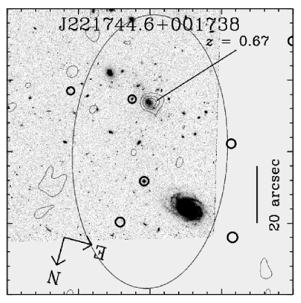
Figure 13: HST F814W image of the region within the extended X-ray source J221744.6+001738 (see $\S$5 for detail). The image itself is 100 arcsec per side. The extent of the X-ray source has been highlighted with the black ellipse, and represents the approximate shape of the extended emission that exceeds $\approx$10 per cent of the local 0.5–2 keV background (determined from the adaptively-smoothed soft-band image; see $\S$3.1). X-ray sources from our main catalog have been highlighted with thick circles, with the size of each circle representing roughly the 90 per cent encircled energy fraction as computed at 1.497 keV. Within the image, a small clustering of galaxies is notable in the southern region (top region) of the extended X-ray emission, which is the likely source of the X-ray emission. Radio (1.4 GHz) contours indicating intensity levels of 2.7, 8.0, 13.3, 18.6, 23.9, and 29.2 $\times 10^{6}$ Jy sr^-1 have been indicated. The most probable cluster central galaxy J221744.3+001722, which is coincident with a bright radio source (1.4 GHz flux of 1.4 mJy) and has a spectroscopic redshift of $z=0.67$, has been highlighted.

Using the above methods, we find $n_{\rm src}=410\pm 37$ soft-band counts; using the average exposure over the extended source $\approx$363 ks, implies a soft-band count-rate of $(1.1\pm 0.1)\times 10^{-3}$ counts s^-1. Figure 13 shows the HST F814W image in the vicinity of the extended X-ray emission. From the image, a small clustering of galaxies is apparent in the southern region of the extraction ellipse, with a few elliptical galaxies residing in the highest density regions. It is therefore plausible that the extended X-ray emission observed in J221744.6+001738 is associated with a group or poor cluster traced by these galaxies. We searched the redshift catalogs discussed in $\S$3.2.3 for obvious redshift spikes; however, due to small number statistics, we were unable to confirm or deny the presence of an overdensity in this region. Using $J-K$ colours, we found that a larger fraction of the galaxies within the extended X-ray emission had “red” [$(J-K)_{\rm Vega}>1.5$] near-IR colours compared with those found over the entire Chandra observed SSA22 field. A K-S test indicates that the distribution of $J-K$ colours in this region are similar only at the $\approx$6 per cent confidence level. The difference in colour distributions is almost certainly due to an excess of “red” galaxies in this region, which indicate $z\approx$ 0.5–1.5 galaxies having notable 4000 Å breaks (e.g., Swinbank et al. 2007). The most likely cluster central galaxy in this region [selected based on visual morphology, location relative to other nearby sources, $K$-band magnitude, and near-IR colour; $(J-K)_{\rm Vega}=2.0$] is J221744.3+001722 (indicated in Fig. 13). This source has been found to have a redshift of $z=0.67$ (from Chapman et al. 2009, in-preparation) and is one of only three sources within the extent of the X-ray emission to have a spectroscopic redshift available. The source is coincident with a bright 1.4 GHz source with a flux density of 1.4 mJy (see contours in Fig. 13; Chapman et al. 2004), which corresponds to a 1.4 GHz luminosity of $\approx$$3\times 10^{24}$ W Hz^-1. Since moderately luminous radio sources like J221744.3+001722 typically trace highly clustered regions (e.g., Wake et al. 2008), this provides further evidence that the extended X-ray emission is likely due to the presence of a group or poor cluster.

Assuming that the extended source is indeed powered by a group or poor cluster at $z=0.67$, we computed the expected soft-band flux and luminosity assuming a Raymond-Smith thermal plasma (Raymond & Smith 1977) with $kT=1.0$ keV and $Z=0.2Z_{\odot}$. This gives a soft-band flux of $(9.5\pm 0.9)\times 10^{-15}$ ergs cm^-2 s^-1 and rest-frame 0.5–2 keV luminosity of $(2.3\pm 0.2)\times 10^{43}$ ergs s^-1. However, to confirm the redshift and the intrinsic X-ray spectral shape of J221744.6+001738 requires a more complete census of galaxy redshifts in this region and more detailed X-ray spectral analyses, which are beyond the scope of this paper.

6 Summary

We have presented point-source catalogs and basic analyses of sources detected in a deep $\approx$400 ks Chandra exposure over a $\approx$330 arcmin² region centred on a $z=3.09$ protocluster in the SSA22 region: The Chandra Deep Protocluster Survey. The survey reaches on-axis flux limits in the 0.5–2 keV and 2–8 keV bandpasses of $\approx$$5.7\times 10^{-17}$ ergs s^-1 and $\approx$$3.0\times 10^{-16}$ ergs s^-1, respectively. We have presented a main Chandra catalog of 297 point sources, which was generated by (1) running wavdetect at a false-positive probability threshold of $10^{-5}$ and (2) filtering this list to include only sources that were determined to have X-ray emission that was significant in comparison to their local backgrounds. In addition to the point sources, we have presented the properties of one 0.5–2 keV extended source, which is likely associated with a group or poor cluster between $z\approx$ 0.5–1. We have cross-correlated our main catalog source positions with near–to–mid-infrared photometry and optical spectroscopic redshift catalogs to determine the nature of the detected point sources. The combined X-ray and multiwavelength data sets indicate a variety of source types, most of which are absorbed AGNs that dominate at lower X-ray fluxes. In total, we have determined that 12 of the main catalog sources are likely associated with the $z=3.09$ protocluster, including sources that have either spectroscopic redshifts between $z=$ 3.06–3.12 and/or sources that are coincident with LAEs. The majority of these sources lie in the highest density regions of the protocluster, and we find evidence that the AGN fraction is positively correlated with local LAE density (96 per cent confidence).

Appendix A Additional wavdetect Sources

In this section, we present the source properties of the additional nine sources excluded from our main Chandra catalog presented in $\S$3.2.2 and Table 2 that were detected by wavdetect at a minimum false-positive probability threshold $\leq$$10^{-6}$. In Table A1, we present the properties of these nine sources. Table A1 has the exact same column structure as Table 2. Columns have the same meaning as they did in Table 2, with one key exception: the counts and errors for X-ray detected sources that are provided in columns (8)–(16) come from wavdetect photometry. A source is considered to be detected in a given band when the source is detected by wavdetect. When a source is not detected in a given band, an upper limit is computed in the same manner as that presented in the description of columns (8)–(16) in Table 2. Columns that make use of columns (8)–(16) (i.e., column 2 and columns 35–43) utilise the values presented here.

These sources are presented at the convenience of the user who wishes to create a purely wavdetect based catalog of X-ray sources. This can be achieved by appending Table A1 to Table 2 and filtering the merged catalog by the desired minimum wavdetect probability presented in column 5 to create a wavdetect catalog with false-positive probability threshold of $10^{-6}$, $10^{-7}$, or $10^{-8}$.

Table 6: Supplementary catalog of additional wavdetect sources with false-positive probability $\leq$$10^{-6}$ that are not in the main Chandra catalog.

	X-ray Coordinates		Detection Probability				Net Counts
Source					Pos. Error	$\theta$
Number	$\alpha_{\rm J2000}$	$\delta_{\rm J2000}$	AE	wavdetect	(arcsec)	(arcmin)	0.5–8 keV	0.5–2 keV	2–8 keV
(1)	(2)	(3)	(4)	(5)	(6)	(7)	(8)–(10)	(11)–(13)	(14)–(16)
1	22 17 02.02	+00 13 32.4	0.953	$-$6	3.31	8.95	7.0$\pm$4.2	$<$19.7	$<$34.8
2	22 17 26.23	+00 19 34.7	0.947	$-$7	1.61	4.82	$<$14.3	4.1$\pm$2.2	$<$11.4
3	22 17 26.93	+00 10 45.2	0.802	$-$6	1.82	5.41	$<$14.6	4.1$\pm$2.2	$<$11.9
4	22 17 28.59	+00 18 25.8	0.914	$-$8	1.13	3.53	4.9$\pm$2.5	$<$7.8	3.7$\pm$2.2
5	22 17 31.02	+00 07 35.2	0.542	$-$6	3.01	8.10	$<$27.0	5.4$\pm$3.0	$<$24.4
6	22 17 36.58	+00 09 11.8	0.977	$-$6	1.59	6.36	11.0$\pm$4.2	$<$9.9	11.1$\pm$4.1
7	22 17 49.43	+00 22 18.2	0.911	$-$6	2.69	7.43	4.9$\pm$4.0	$<$18.0	$<$24.7
8	22 18 01.13	+00 24 57.7	0.660	$-$6	5.45	11.20	7.0$\pm$3.9	$<$19.5	15.9$\pm$6.4
9	22 18 08.90	+00 08 40.5	0.887	$-$6	2.49	10.57	42.8$\pm$10.4	$<$23.3	$<$39.5

NOTE. — Table A1 is presented in its entirety in the electronic version; an abbreviated version of the table is shown here for guidance as to its form and content. The full table contains 44 columns of information for the nine sources. Meanings and units for all columns have been summarized in detail in $\S\S$ 3.2.2 and Appendix A.

References

- Alexander et al. (2001) Alexander, D. M., Brandt, W. N., Hornschemeier, A. E., Garmire, G. P., Schneider, D. P., Bauer, F. E., & Griffiths, R. E. 2001, AJ, 122, 2156
- Alexander et al. (2003) Alexander, D. M., et al. 2003, AJ, 126, 539
- Baganoff et al. (2003) Baganoff, F. K., et al. 2003, ApJ, 591, 891
- Boller et al. (1998) Boller, Th., Bertoldi, F., Dennefeld, M., & Voges, W. 1998, A&AS, 129, 87
- Bower et al. (2004) Bower, R. G., et al. 2004, MNRAS, 351, 63
- Brandt & Hasinger (2005) Brandt, W. N., & Hasinger, G. 2005, ARA&A, 43, 827
- Broos et al. (2000) Broos, P., et al. 2000, User’s Guide for the TARA Package. (University Park: Pennsylvania State Univ.)
- Broos et al. (2002) Broos, P. S., Townsley, L. K., Getman, K., & Bauer, F. E. 2002, ACIS Extract, An ACIS Point Source Extraction Package (University Park: Pennsylvania State Univ.)
- Chapman et al. (2001) Chapman, S. C., Lewis, G. F., Scott, D., Richards, E., Borys, C., Steidel, C. C., Adelberger, K. L., & Shapley, A. E. 2001, ApJL, 548, L17
- Chapman et al. (2004) Chapman, S. C., Scott, D., Windhorst, R. A., Frayer, D. T., Borys, C., Lewis, G. F., & Ivison, R. J. 2004, ApJ, 606, 85
- De Lucia et al. (2006) De Lucia, G., Springel, V., White, S. D. M., Croton, D., & Kauffmann, G. 2006, MNRAS, 366, 499
- Donley et al. (2008) Donley, J. L., Rieke, G. H., Pérez-González, P. G., & Barro, G. 2008, ApJ, 687, 111
- Feigelson et al. (2000) Feigelson, E.D., Broos, P.S., & Gaffney, J. 2000, Memo on the Optimal Extraction Radius for ACIS Point Sources. The Pennsylvania State University, University Park
- Freeman et al. (2002) Freeman, P.E., Kashyap, V., Rosner, R., & Lamb, D.Q. 2002, ApJS, 138, 185
- Garilli et al. (2008) Garilli, B., et al. 2008, A&A, 486, 683
- Garmire et al. (2003) Garmire, G. P., Bautz, M. W., Ford, P. G., Nousek, J. A., & Ricker, G. R. 2003, Proc. SPIE, 4851, 28
- Geach et al. (2005) Geach, J. E., et al. 2005, MNRAS, 363, 1398
- Geach et al. (2009) Geach, J. E., et al. 2009, ApJ, in-press (astro-ph/0904.0452)
- Gebhardt et al. (2000) Gebhardt, K., et al. 2000, ApJL, 539, L13
- Gehrels (1986) Gehrels, N. 1986, ApJ, 303, 336
- Gendreau et al. (1995) Gendreau, K. C. et al. 1995, PASJ, 47, L5
- Georgakakis et al. (2008) Georgakakis, A., Nandra, K., Laird, E. S., Aird, J., & Trichas, M. 2008, MNRAS, 388, 1205
- Getman et al. (2005) Getman, K. V., et al. 2005, ApJS, 160, 319
- Governato et al. (1998) Governato, F., Baugh, C. M., Frenk, C. S., Cole, S., Lacey, C. G., Quinn, T., & Stadel, J. 1998, Nature, 392, 359
- Hayashino et al. (2004) Hayashino, T., et al. 2004, AJ, 128, 2073
- Hickox & Markevitch (2006) Hickox, R. C., & Markevitch, M. 2006, ApJ, 645, 95
- Hornschemeier et al. (2001) Hornschemeier, A.E., et al. 2001, ApJ, 554, 742
- Hornschemeier et al. (2004) Hornschemeier, A. E., et al. 2004, ApJL, 600, L147
- Jerius et al. (2000) Jerius, D., Donnelly, R.H., Tibbetts, M.S., Edgar, R.J., Gaetz, T.J., Schwartz, D.A., Van Speybroeck, L.P., & Zhao, P. 2000, Proc. SPIE, 4012, 17
- Kauffmann (1996) Kauffmann, G. 1996, MNRAS, 281, 487
- Kim et al. (2006) Kim, D.-W., et al. 2006, ApJ, 644, 829
- Kim et al. (2007) Kim, M., et al. 2007, ApJS, 169, 401
- Lacy et al. (2004) Lacy, M., et al. 2004, ApJS, 154, 166
- Laird et al. (2009) Laird, E. S., et al. 2009, ApJS, 180, 102
- Lawrence et al. (2007) Lawrence, A., et al. 2007, MNRAS, 379, 1599
- Le Fèvre et al. (2005) Le Fèvre, O., et al. 2005, A&A, 439, 845
- Lehmer et al. (2005) Lehmer, B. D., et al. 2005, ApJS, 161, 21
- Lehmer et al. (2006) Lehmer, B. D., et al. 2006, AJ, 131, 2394
- Lehmer et al. (2007) Lehmer, B. D., et al. 2007, ApJ, 657, 681
- Lehmer et al. (2008) Lehmer, B. D., et al. 2008, ApJ, 681, 1163
- Lehmer et al. (2009) Lehmer, B. D., et al. 2009, ApJ, 691, 687
- Luo et al. (2008) Luo, B., et al. 2008, ApJS, 179, 19
- Markevitch et al. (2001) Markevitch, M. 2001, CXC memo (http://asc.harvard.edu/cal/)
- Markevitch et al. (2003) Markevitch, M., et al. 2003, ApJ, 583, 70
- Marshall et al. (1980) Marshall, F. E., Boldt, E. A., Holt, S. S., Miller, R. B., Mushotzky, R. F., Rose, L. A., Rothschild, R. E., & Serlemitsos, P. J. 1980, ApJ, 235, 4
- Matsuda et al. (2004) Matsuda, Y., et al. 2004, AJ, 128, 569
- Matsuda et al. (2005) Matsuda, Y., et al. 2005, ApJL, 634, L125
- Nandra et al. (2005) Nandra, K., et al. 2005, MNRAS, 356, 568
- Ptak et al. (2007) Ptak, A., Mobasher, B., Hornschemeier, A., Bauer, F., & Norman, C. 2007, ApJ, 667, 826
- Raymond & Smith (1977) Raymond, J. C., & Smith, B. W. 1977, ApJS, 35, 419
- Richards et al. (2006) Richards, G. T., et al. 2006, ApJS, 166, 470
- Spergel et al. (2003) Spergel, D. N., et al. 2003, ApJS, 148, 175
- Stark et al. (1992) Stark, A. A., Gammie, C. F., Wilson, R. W., Bally, J., Linke, R. A., Heiles, C., & Hurwitz, M. 1992, ApJS, 79, 77
- Steidel et al. (1998) Steidel, C. C., Adelberger, K. L., Dickinson, M., Giavalisco, M., Pettini, M., & Kellogg, M. 1998, ApJ, 492, 428
- Steidel et al. (2000) Steidel, C. C., Adelberger, K. L., Shapley, A. E., Pettini, M., Dickinson, M., & Giavalisco, M. 2000, ApJ, 532, 170
- Steidel et al. (2003) Steidel, C. C., Adelberger, K. L., Shapley, A. E., Pettini, M., Dickinson, M., & Giavalisco, M. 2003, ApJ, 592, 728
- Swinbank et al. (2007) Swinbank, A. M., et al. 2007, MNRAS, 379, 1343
- Tamura et al. (2009) Tamura, Y., et al. 2009, Nature, 459, 61
- Townsley et al. (2000) Townsley, L.K., Broos, P.S., Garmire, G.P., & Nousek, J.A. 2000, ApJ, 534, L139
- Townsley et al. (2002) Townsley, L.K., Broos, P.S., Nousek, J.A., & Garmire, G.P. 2002, Nuclear Instruments and Methods in Physics Research A, 486, 751
- Tozzi et al. (2006) Tozzi, P., et al. 2006, A&A, 451, 457
- Uchimoto et al. (2008) Uchimoto, Y. K., et al. 2008, PASJ, 60, 683
- Vikhlinin et al. (1995) Vikhlinin, A., Forman, W., Jones, C., & Murray, S. 1995, ApJ, 451, 553
- Vikhlinin et al. (2001) Vikhlinin, A. 2001, CXC Memo, (Cambridge: CXC) http://asc.harvard.edu/cal/Acis/Cal_prods/vfbkgrnd/
- Wake et al. (2008) Wake, D. A., Croom, S. M., Sadler, E. M., & Johnston, H. M. 2008, MNRAS, 391, 1674
- Webb et al. (2009) Webb, T. M. A., Yamada, T., Huang, J.-S., Ashby, M. L. N., Matsuda, Y., Egami, E., Gonzalez, M., & Hayashimo, T. 2009, ApJ, 692, 1561
- Weisskopf et al. (2007) Weisskopf, M. C., Wu, K., Trimble, V., O’Dell, S. L., Elsner, R. F., Zavlin, V. E., & Kouveliotou, C. 2007, ApJ, 657, 1026
- Wilman et al. (2005) Wilman, R. J., Gerssen, J., Bower, R. G., Morris, S. L., Bacon, R., de Zeeuw, P. T., & Davies, R. L. 2005, Nature, 436, 227
- Worsley et al. (2005) Worsley, M. A., et al. 2005, MNRAS, 357, 1281