Chandra Observations of 1RXS J141256.0+792204 (Calvera)

Abstract

We report the results of a 30 ks Chandra/ACIS-S observation of the isolated compact object 1RXS J141256.0+792204 (Calvera). The X-ray spectrum is adequately described by an absorbed neutron star hydrogen atmosphere model with $\mbox{$kT_{\rm eff}^{\infty}$}=88.3\pm 0.8$ eV and radiation radius $R^{\infty}/d=4.1\pm 0.1$ km kpc^-1. The best-fit blackbody spectrum yields parameters consistent with previous measurements; although the fit itself is not statistically acceptable, systematic uncertainties in the pile-up correction may contribute to this. We find marginal evidence for narrow spectral features in the X-ray spectrum between 0.3 and 1.0 keV. In one interpretation, we find evidence at 81%-confidence for an absorption edge at $E=0.64\mbox{${}^{+0.08}_{-0.06}$}$ keV with equivalent width ${\rm EW}\approx 70$ eV; if this feature is real, it is reminiscent of features seen in the isolated neutron stars RX J1605.3+3249, RX J0720.4$-$3125, and 1RXS J130848.6+212708 (RBS 1223). In an alternative approach, we find evidence at 88% -confidence for an unresolved emission line at energy $E=0.53\pm 0.02$ keV, with equivalent width ${\rm EW}\approx 28$ eV; the interpretation of this feature, if real, is uncertain. We search for coherent pulsations up to the Nyquist frequency $\mbox{$\nu_{\rm Nyq}$}=1.13$ Hz and set an upper limit of 8.0% rms on the strength of any such modulation. We derive an improved position for the source and set the most rigorous limits to-date on any associated extended emission on arcsecond scales. Our analysis confirms the basic picture of Calvera as the first isolated compact object in the ROSAT/Bright Source Catalog discovered in six years, the hottest such object known, and an intriguing target for multiwavelength study.

1 Introduction

Between 1996 and 2001, seven of the 18,811 sources in the ROSAT Bright Source Catalog (BSC; Voges et al. 1999) were identified as radio-quiet neutron stars without associated supernova remnants or binary companions. These seven isolated neutron stars (INSs; Haberl 2005) have the following properties: X-ray-to-optical flux ratios exceeding 1000, thermal spectra peaking in the far-UV or soft X-ray, minimal ($<$10%) long-term X-ray variability, and rotation periods of several seconds. These properties are consistent with interpretation of the INSs as a population of $\sim$Myr-old, cooling, non-accretion-powered neutron stars.

The spectra of INSs show little evidence of non-thermal emission, with atmospheres that are thought to be well-suited for theoretical modeling (Rajagopal & Romani, 1996; Pavlov et al., 1996) that may ultimately lead to constraints on neutron star physical parameters and the equation of state (EOS; Lattimer & Prakash 2004; Page et al. 2006). However, the true EOS cannot be distinguished from among the plethora of possible EOSs consistent with current theories of quantum chromodynamics without multiple data points (van Kerkwijk, 2003), and a sample of seven is likely too small to effectively solve this puzzle.

For more than six years, and despite substantial efforts (e.g., Rutledge et al. 2003; Agüeros et al. 2006), no new INSs were discovered in the BSC. In 2005 we initiated a new approach to this problem, identifying BSC sources likely to have high X-ray-to-optical flux ratios and using NASA’s Swift satellite (Gehrels et al., 2004) to efficiently survey these targets (see Fox 2004; Shevchuk et al. in prep; Letcavage et al. in prep). Based on the results of our survey effort, now substantially complete, Turner et al. (2009) estimate that the BSC contains fewer than 48 INSs at 90% confidence, assuming all-sky isotropy. As such, the BSC in total may provide only a modest increase in the number of known INSs; nonetheless, it remains a promising catalog to explore for these objects. At fainter flux levels, a strong candidate INS, 2XMM J104608.7$-$594306, has recently been discovered with XMM-Newton, and discovery of more such objects may be anticipated in the future (Pires et al., 2009).

The first confirmed isolated compact object (ICO) from our survey of BSC sources is 1RXS J141256.0+792204 (Calvera). Initial observations of Calvera left substantial room for interpretation (Rutledge et al., 2008). Calvera’s temperature, as determined by a blackbody model of the Swift spectrum, is $215\pm{25}$ eV, approximately twice that of 1RXS J130848.6+212708, the hottest previously-known INS. Combined with its Galactic latitude of 37^∘, Calvera must be $\approx$5 kpc above the Galactic plane to conform to the INS model. Current cooling models suggest it is not feasible for a neutron star to move so far from its (likely) origin in the Galactic plane while remaining so hot, which casts doubt on Calvera’s interpretation as an INS. Searching for a way to frame the Swift results in the context of known neutron star classes, it was suggested that Calvera might be a millisecond radio pulsar (MSP) at a distance of 80–260 pc from the Sun (Rutledge et al., 2008). This claim was based on an exploration of a range of possible distances and (corresponding) X-ray luminosities for Calvera, which – for reasonable distance values – yielded consistent results only in comparison to the properties of the 47 Tuc MSP population. Subsequent radio observations yielded no evidence of radio pulsations to deep luminosity limits (Hessels et al., 2007), suggesting that if Calvera is a nearby radio MSP, it is beamed away from Earth.

The aim of the present work is to examine Calvera’s X-ray properties via our recent 30 ks Chandra ACIS-S observation, the most detailed investigation of the source to-date. In §2 we discuss the parameters of this observation, our analysis, and the models used to interpret the data, addressing in turn the astrometric, spatial, timing, and spectroscopic implications of the Chandra data. §3 discusses these results in the larger context of INS studies, and §4 summarizes our conclusions.

2 Observations & Analysis

Data were analyzed using CIAO v4.0.1 (Fruscione et al., 2006) with Chandra calibration database CALDB v3.4.4.

Chandra observed 1RXS J141256.0+792204 with the ACIS-S detector beginning 8 Apr 2008 03:42:08 TT, in a single pointing. The standard 1/8 subarray was used, giving a time resolution of 0.44104 s, with the target placed at the center of the subarray window and offset from the boundary between readout quadrants, according to usual practice. Based on the observed source count rate ($\sim$0.2 ${\rm cts}\,{\rm s^{-1}}$), and accounting for 9.3% deadtime per frame, we observe 0.080 ${\rm cts}\,{\rm frame^{-1}}$. Given this per-frame count rate, a mild level of pile-up is anticipated (see §2.4), which will affect the source spectrum and PSF profile.

The total observation time was 29,142 s; due to CCD read-out, the total exposure time for the observation was 9.3% less, with 26,430 s of exposure (indeed, a small number of “out of time” events are observed in the data). The focal plane temperature was 153.28 K ($-119.87\hbox{${}^{\circ}$}$ C).

Using wavdetect we detect 1RXS J141256.0+792204 with a source detection significance of 72$\sigma$.

2.1 Astrometry

Using uncorrected Chandra astrometry, we localize Calvera to R.A. 14h12m55.84s, Dec. +79d22m03.75s (J2000) with 0.6^′′ radius (90% confidence) uncertainty. This is within the 90% confidence region of the previously-derived X-ray position (Rutledge et al., 2008).

Using previously-analyzed Gemini-North + GMOS imaging of this region (Rutledge et al., 2008), we identify optical counterparts to two X-ray sources in the Chandra field of view, CXOU J141220.78+792251.6 and CXOU J141246.23+792222.3. The two registration sources provide a weighted average correction to the Chandra native coordinates of $\Delta\alpha=-0.21\mbox{$\pm$}0.14\hbox{${}^{\prime\prime}$}$, $\Delta\delta=-0.33\mbox{$\pm$}0.12\hbox{${}^{\prime\prime}$}$, where 1$\sigma$ uncertainties in the correction are dominated by Chandra centroid uncertainties for these faint sources. Applying this correction yields our best estimate for the position of Calvera: R.A.=14h12m55.76s, Dec.=+79:22:03.4 (J2000) with 90%-confidence ellipse semimajor axes of 0.31^′′ (R.A.) $\times$ 0.25^′′ (Dec.), aligned with the coordinate axes.

The brightest X-ray source apart from Calvera is a 5.3$\sigma$ wavdetect detection at R.A. 14h12m52.46s, Dec. +79d21m52.6s (J2000), which has a statistical localization uncertainty of 0.1^′′. This source does not have an optical counterpart in our Gemini imaging; however, its relative brightness would allow it to be used in an X-ray proper motion study. The offset between Calvera and CXOU J141252.46+792152.6 is 14.5$\pm$0.2^′′, which would allow a (3$\sigma$) detection of relative proper motion between the two sources for relative on-sky motions of

$$v_{\rm sky}>290\left(\frac{d_{\rm 100\,pc}}{T_{\rm 1\,yr}}\right)\hbox{${\rm km}\,{\rm s^{-1}}$},$$

where $d_{\rm 100\,pc}$ is the distance to Calvera in units of 100 pc and $T_{\rm 1\,yr}$ is the elapsed time to the second-epoch observation, in years. This limiting velocity corresponds to $v_{\rm calvera}\approx 32,000$ ${\rm km}\,{\rm s^{-1}}$ at a distance of 11 kpc, the distance implied for an INS interpretation of Calvera.

2.2 Spatial Analysis

In order to compare the observed spatial distribution of detected X-ray photons to point-spread-function (PSF) models, we used the Chandra Ray Tracer (ChaRT) with MARX v4.3 (Carter et al., 2003) to produce a ray-trace onto the detector plane using our best-fit X-ray spectrum over the 0.3–8.0 keV photon energy range, using the default internal model for dither-blur and a dither-blur radius of 0.35^′′.

Comparison of the radial count distributions of the observed and simulated (MARX) datasets reveals that the observed distribution is significantly narrower than the MARX distribution, such that the simulated PSF does not provide a statistically acceptable description of the observed PSF, as evaluated with a two-sample K-S test (Press et al., 1995). We interpret this as implying that the X-ray source remains unresolved at Chandra spatial resolution, to within existing Chandra PSF modeling capabilities.

To derive limits on the fractional flux in any resolved component, we simulated added Gaussian spatial components with widths of $\sigma$=1^′′, 5^′′, and 10^′′, respectively. For each specified width, we add counts to the source image until the radial distribution of counts is inconsistent with (and broader than) the observed radial distribution of counts, at 90% confidence, according to a K-S test. In this manner, we produce 90%-confidence upper limits on the fractional flux of any spatially-resolved component. These limits are: $<$5% for $\sigma=1\hbox{${}^{\prime\prime}$}$, and $<$3% for $\sigma=5\hbox{${}^{\prime\prime}$}$ and $\sigma=10\hbox{${}^{\prime\prime}$}$.

2.3 Timing Analysis

We extracted counts within a circle 5^′′ of Calvera, and use a 300 pixel by 70 pixel off-source region to sample background counts, finding 3761 total counts. In the source region for Calvera we detect 4958 counts, giving a background-subtracted count rate of 185$\pm$3 ${\rm cts}\,{\rm ks^{-1}}$. The background represents 1.1% of detected counts and is neglected in the following analysis.

We barycenter-corrected the data using axbary. Using counts at energies $<$5 keV, we produce a power density spectrum with frequencies between 3.4$\times 10^{-5}$ Hz and 1.13 Hz, finding no evidence for periodicity in these data, with a maximum Leahy-normalized power (Leahy et al., 1983) of 20.2. We set a 90%-confidence upper-limit (Vaughan et al., 1994) on the root-mean-square variability for a sinusoidal signal in this frequency range:

$${\rm rms}<\sqrt{\frac{P}{N_{\rm phot}}}\frac{I}{I-B},$$

where $P$ is the upper limit on the detected power, $N_{\rm phot}$ is the number of photons, and $I$ and $B$ are the relative source and background count rates, respectively. Our limit corresponds to ${\rm rms}<8.0\%$ variability. Given that 1RXS J185635.1$-$375433 is known to have pulsations at the 1.2% rms level (Tiengo & Mereghetti, 2007), this may not be considered a strong constraint.

We performed the same analysis for all counts with energies $<$1 keV (2994 counts), and detect no periodicity, with a maximum power of 18.4; the rms upper-limit in this energy range is ${\rm rms}<9.0\%$ ($<$1 keV).

2.4 Spectral Analysis

Spectral analysis was performed with XSPEC v12.3.1x (Arnaud, 1996). Working from the psextract science thread on the Chandra X-ray Center website, we used psextract with a source aperture of 3.7^′′ to extract 4,711 source region counts and two circular background regions on opposing sides of the source, each with radius 30^′′, to extract a total of 158 background counts. The charge bleed upon readout present around the source prevented us from using an annular extraction region. We used mkacisrmf to generate the response matrix and mkarf was then used to generate the ancillary response file. We grouped the spectrum into bins with a minimum of fifty counts per bin over the range 0.32 to 7.33 keV (the maximum detected photon energy).

Using the PIMMS software tool we estimate a pile-up fraction of 3% for this observation. We account for this level of pile-up in our analyses using the pileup model in XSPEC (Davis, 2001), with pile-up model values frozen at values recommended in the Chandra ABC Guide to Pileup: the per-frame integration time is 0.40 s (appropriate to our 1/8-subarray dataset), a maximum of five piled-up photons are modeled, the grade correction parameter g0 is unity, the grade migration parameter $\alpha=0.5$, the PSF fraction is 0.95, and the number of regions used is one. The PSF fraction parameter should equal the fraction of all extracted counts that land in the central 3$\times$3 pixel island, which we find is an appropriate estimate for Calvera; the meaning of the other model parameters is discussed in detail in Davis (2001). As discussed below, we find that this pile-up model can account for the high-energy portion of the observed data for reasonable models of the underlying source spectrum.

All uncertainties below are quoted at 90%-confidence unless otherwise specified.

Power-Law. We find that a power-law spectrum does not provide an adequate fit to the data ($\mbox{$\chi^{2}_{\nu}$}=2.31$ for $\nu=67$ degrees of freedom; $p=7.3\times 10^{-9}$). Incorporating pile-up corrections and allowing the interstellar absorption column to vary freely, we find a best-fit photon index $\alpha=4.8$ with $\mbox{$N_{\rm H}$}=3.4\times 10^{21}$ cm^-2, in excess of the total Galactic column along the line of sight ($\mbox{$N_{\rm H}$}=2.65\times 10^{20}$ cm^-2 from H I maps; Kalberla et al. 2005).

Blackbody. We find that a blackbody spectrum does not fit the data acceptably ($\mbox{$\chi^{2}_{\nu}$}=2.04$ for $\nu=67$ degrees of freedom, $p=1.0\times 10^{-6}$). The best-fit temperature for a blackbody with pile-up corrections and without interstellar absorption (the equivalent neutral hydrogen column density $N_{\rm H}$, a free parameter, is driven to zero during the fit) is $kT=229$ eV, with blackbody normalization $(R_{\rm km}/D_{\rm 10\,kpc})^{2}=26.6$. This fit is consistent with our original Swift XRT observation, which yielded $kT=215\pm 25$ eV (Rutledge et al., 2008). For reference purposes only, we present the parameters of our best-fit blackbody (without uncertainties, as these are not well defined in the absence of an acceptable fit) in Table 1.

Neutron Star Hydrogen Atmosphere. Fitting the spectrum of a neutron star hydrogen atmosphere model (nsa model component in XSPEC; Zavlin et al. 1996), including interstellar absorption and pile-up corrections, yields a fit with $\mbox{$\chi^{2}_{\nu}$}=1.305$ ($\nu=67$) and best-fit parameters: effective temperature $kT_{\rm eff}=109\pm 1$ eV, equivalent neutral hydrogen column density $N_{H}=3.1\pm 0.9\times 10^{20}$ cm^-2, and normalization $D_{\rm kpc}^{-2}=0.077_{-0.038}^{+0.041}$. In using the nsa model we fix the neutron star mass at 1.4 $M_{\odot}$, its radius at 12 ${\rm km}$, and its magnetic field at zero; since this neutron star model gives a gravitational redshift of $z_{g}=0.235$, the corresponding parameters for distant observers are $\mbox{$kT_{\rm eff}^{\infty}$}=88.3\pm 0.8$ eV, $R^{\infty}=14.8$ km, and $R^{\infty}/d=4.1\pm 0.1$ km kpc^-1.

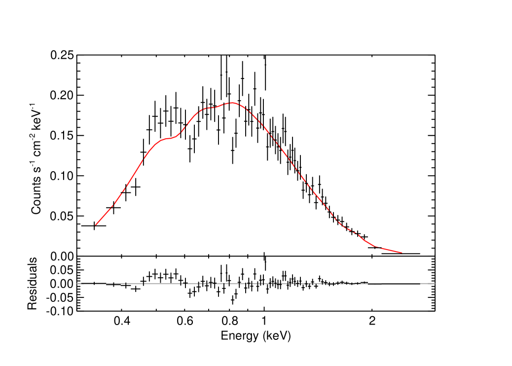
Figure 1: The X-ray spectrum of Calvera (data), folded through the ACIS-S response matrix and shown with our best-fit model (red line) and residuals (lower panel). The model consists of a non-magnetized neutron star hydrogen atmosphere with gravitational mass $M=1.4\mbox{$M_{\odot}$}$ and physical radius $R=12$ km fixed, and having $kT_{\rm eff}=109\pm 1$ eV, normalization $D_{\rm kpc}^{-2}=7.71^{+0.41}_{-0.38}\times 10^{-2}\,$, Galactic absorption $\mbox{$N_{\rm H}$}=3.1\pm 0.9\times 10^{20}$ cm^-2, and pile-up corrections (see text for details). Data have been binned to a minimum of 50 source counts per bin. The best-fit spectrum is statistically acceptable ($\mbox{$\chi^{2}_{\nu}$}=1.305$ for $\nu=67$, giving a probability of 4.9%), but some systematic trends in the fit residuals can be seen. The most statistically significant of these corresponds to a possible absorption feature at $E\approx 0.64$ keV, or emission feature at $E\approx 0.53$ keV, as discussed in the text.

This fit can be seen in Fig. 1; the systematic trends in the residuals below $E\approx 1$ keV are suggestive and motivate investigation of models with additional components.

Neutron Star Hydrogen Atmosphere + Absorption Edge. Attempts to fit the spectrum with an unresolved absorption line at $E\approx 0.65$ keV did not achieve stable results. However, fitting the spectrum with a neutron star hydrogen atmosphere model plus absorption edge (edge and nsa models in XSPEC), including interstellar absorption and pile-up corrections, yields $\mbox{$\chi^{2}_{\nu}$}=1.188$ ($\nu=65$). This model has best-fit parameters: effective temperature $kT_{\rm eff}=109\pm 1$ eV, equivalent neutral hydrogen column density $N_{H}=3.4\pm 0.8\times 10^{20}$ cm^-2, and normalization $D_{\rm kpc}^{-2}=0.079$. The edge has best-fit parameters of energy $E_{\rm edge}=0.64^{+0.08}_{-0.06}$ keV and depth $\tau_{\rm edge}=0.28\pm 0.12$ (Table 1), corresponding to an equivalent width of ${\rm EW}\approx 70$ eV. The neutron star mass, radius, and magnetic field are fixed as before.

The addition of the edge feature results in a noticeable improvement in the fit, $\Delta\mbox{$\chi^{2}$}=10.1$, but we do not consider this improvement significant for the reasons discussed below.

Neutron Star Hydrogen Atmosphere + Gaussian Emission Line. We also investigated an emission-line interpretation for the low-energy residuals. We find that an unresolved (width frozen at zero) emission line (gaussian model in XSPEC) added to the hydrogen atmosphere model, including appropriate $N_{\rm H}$ absorption and pile-up corrections, is statistically preferred to the absorption edge fit. With $\mbox{$\chi^{2}_{\nu}$}=1.158$ ($\nu=65$), the model best-fit parameters are $kT_{\rm eff}=122\pm 3$ eV, $N_{H}=1.5\pm 1.0\times 10^{20}$ cm^-2, and normalization $D_{\rm kpc}^{-2}=0.041$. The line energy is $E_{\rm line}=0.53\pm 0.02$ keV with a normalization of $2.48^{+1.4}_{-1.1}\times 10^{-5}$ photon cm^-2 s^-1, corresponding to an equivalent width of ${\rm EW}\approx 28$ eV. Other nsa parameters remain fixed as before.

The addition of the emission line component provides an improvement of $\Delta\mbox{$\chi^{2}$}=12.2$, and is thus statistically preferred to the absorption edge fit. As we show below, however, it also falls short of the 3$\sigma$ threshold that we would require to report detection.

2.5 Monte Carlo Analyses

In order to investigate the statistical significance of the possible low-energy absorption / emission features, and to estimate confidence intervals on model parameters, we have carried out several Monte Carlo analyses of the Calvera spectroscopic dataset.

To generate confidence intervals (Table 1), we perform a bootstrap Monte Carlo analysis (Press et al., 1995). Drawing with replacement from the photons making up our observed spectrum of Calvera, we generate 10,000 bootstrap realizations of the spectrum, fitting each realization with the spectral models described above. We perturb the start parameters for each fit randomly, according to preliminary estimates of the parameter uncertainties, in order to assure exploration of the $\chi^{2}$ landscape near minimum in every case. Typical final $\chi^{2}$ values for these automated fits are higher than derived for the original data, as expected if the fits fail to identify the global minimum for each dataset. In the present application, this can be expected to increase our estimates of parameter uncertainties, yielding conservative estimates, and so is not a significant concern. Our quoted confidence intervals are defined as the minimum-length intervals providing coverage of the appropriate fraction of parameter values from these bootstrap trials.

To evaluate the statistical significance of the low-energy spectral features, we generate a fake spectrum using the parameters of our best-fit pure hydrogen atmosphere model and having the same number of photons as the Calvera spectrum. We use this spectrum for a bootstrap Monte Carlo analysis, generating $\approx$10,000 bootstrap realizations of a Calvera-like spectrum that is now known to exhibit no edge or line feature at low energies. For each spectrum, we perform a series of fits within XSPEC (after randomly perturbing the parameter starting values, as previously). First, we find the best-fit hydrogen atmosphere spectrum. Next, for a series of prospective edge or line energies running from 0.3 keV to 2.0 keV, in 0.1 keV increments, we fit a hydrogen atmosphere + absorption edge (or emission line) model. The difference between the $\chi^{2}$ value of the best-fit no-feature spectrum and the minimum $\chi^{2}$ value from fits incorporating an absorption edge or emission line (of any energy) is then recorded as the $\Delta\chi^{2}$ improvement for that realization. We treat the resulting distribution of $\Delta\chi^{2}$ values as the distribution of a test statistic, in order to evaluate the probability of the null hypothesis that there is no absorption edge (or emission line) present in the actual spectrum of Calvera.

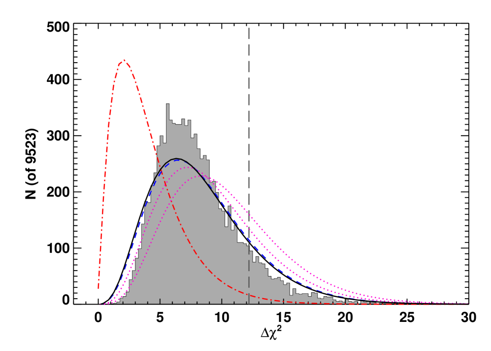
Figure 2: Distribution of $\Delta\chi^{2}$ values from our bootstrap Monte Carlo analysis of the Calvera spectrum (histogram). For each of 9,523 bootstrap realizations of a “fake” Calvera spectrum, known not to exhibit an emission line, we calculate the difference in $\chi^{2}$ values between the best-fit line and no-line models. We then use this distribution as a test-statistic to evaluate the significance of $\Delta\chi^{2}=12.2$, as observed for the actual Calvera spectrum (vertical dashed line). Our analysis suggests detection at 88%-confidence and we conclude that the emission line is not a statistically significant feature; an alternative absorption edge interpretation is supported at 80%-confidence in a similar analysis. Also shown on this plot are the $\chi^{2}$ distribution that best fits the histogram of bootstrap values (black line, for $\nu=8.38$ degrees of freedom), and the distributions predicted by several realizations of Occam’s Razor as applied to our analysis: the Akaike criterion (red dash-dotted line, $\nu=4$); the Bayesian Information Criterion (blue dashed line, $\nu=8.47$); and two realizations of the Sorkin criterion (magenta dotted lines, $\nu=9.21$ and $\nu=10.27$). See text for detailed discussion.

The distribution of $\Delta\chi^{2}$ values from our bootstrap Monte Carlo analysis for the emission line is shown in Fig. 2. Since $\Delta\chi^{2}=12.2$ for the actual Calvera spectrum, we find the null hypothesis is disfavored at the $p=0.12$ or 88%-confidence level, i.e., the improvement in fit is not statistically significant. The results for the absorption edge, which provides $\Delta\chi^{2}=10.1$ for the actual data set, show that the null hypothesis in this case is disfavored at the $p=0.19$ or 81%-confidence level.

We note that these relatively low significance values are due in part to our inability to specify the energy of the strongest absorption feature or emission line a priori.

3 Discussion

Our 30 ks Chandra + ACIS-S observation of Calvera has served to confirm the ICO nature of this source, by several means. First, we have confirmed the non-variable nature of Calvera on short ($10^{-4}\,{\rm Hz}\mathrel{\hbox{\hbox to0.0pt{\hbox{\lower 4.0pt\hbox{$\sim$}}\hss}\hbox{$<$}}}\nu<1.13$ Hz) and long ($>$year) time-scales. Second, we have shown for the first time that a blackbody fit is not adequate to explain the emergent spectrum of Calvera over 0.3 to 7.0 keV; rather, a neutron star hydrogen atmosphere model, with possible additional components, is required. Third, the source retains its point-source appearance in this deepest high-resolution X-ray observation to-date.

Our observations do not resolve the fundamental conundrum of interpretation for this source, first presented in Rutledge et al. (2008). Indeed, this conundrum is sharpened by our NS atmosphere fits, which imply a distance of 3.6 kpc (=$1/\sqrt{D_{\rm kpc}^{-2}}$; see Table  1) for Calvera if its surface X-ray emission is nearly uniform, as in an INS scenario. Our measured column density, $\mbox{$N_{\rm H}$}=3.1\pm 0.9\times 10^{20}$ cm^-2, is consistent with the total Galactic column in the direction of Calvera, estimated at $\mbox{$N_{\rm H}$}=2.65\times 10^{20}$ cm^-2 from H I maps (Kalberla et al., 2005).

The absence of slow X-ray pulsations, to our limit of 8.0% rms, serves as a new and distinct aspect in which Calvera differs from most (though not all) members of the INS population. The frequency range of the present search leaves the possibility of fast ($\nu\mathrel{\hbox{\hbox to0.0pt{\hbox{\lower 4.0pt\hbox{$\sim$}}\hss}\hbox{$>$}}}1$ Hz) X-ray pulsations untested; at the same time, the search sensitivity is not sufficient to rule out low-amplitude, slow pulsations such as those observed from 1RXS J185635.1$-$375433 (Tiengo & Mereghetti, 2007). If Calvera is close to the Galactic plane, as expected given its relatively high temperature, then it must exhibit non-uniform surface emission which, in turn, is expected to produce X-ray pulsations at some level.

3.1 Spectrum

Absorption features in the 0.1 to 1.0 keV energy range have been observed, with varying degrees of significance, in a majority of INSs at this point (see Haberl 2005; Weisskopf et al. 2007; and references therein). The interpretation of these features remains unclear. However, observation of multiple features in at least three INSs, with energies lying in (or close to) harmonic relationships (e.g., at energies 0.7 and 1.4 keV for 1E 1207.4$-$5209; Sanwal et al. 2002), has led to their proposed interpretation as cyclotron resonances of protons or electrons in the neutron star atmosphere. Alternatively, it has been argued that they may reflect atomic features of highly-ionized atmospheric helium, oxygen, or neon (Sanwal et al., 2002; Mori & Ho, 2007).

If the possible absorption feature identified in our spectrum of Calvera is real, then its properties are reminiscent of the known INS absorption features, with the relatively higher energy $E\approx 640$ eV suggesting a correspondingly stronger magnetic field in a cyclotron interpretation.

Moreover, we note that photons with energies below 0.3 keV have been excluded from our spectral analysis, as the ACIS response at these energies is uncalibrated. Examination of the spatial distribution of lower-energy photons, however, leaves no doubt that Calvera is detected as a point source down to $E\approx 0.1$ keV. As such, it is possible that an X-ray spectral analysis of the broad range of 0.1–5.0 keV emission from Calvera at high signal-to-noise will reveal absorption features at lower energies. As a corollary, such an analysis might show our present estimate of the column density to Calvera to have been biased high by the presence of discrete (intrinsic) absorption near 0.3 keV.

3.2 On Occam’s Razor

Detection of discrete features in X-ray spectra requires adding at least two parameters (the feature energy and its depth or normalization) to any underlying spectral model. The question of whether the subsequent improvement in the fit statistic is significant, given the number of added parameters, is properly treated as an Occam’s Razor problem (see, e.g., Magueijo & Sorkin 2007 and references therein).

Quantitatively, Occam’s Razor seeks to minimize the sum of the information content of the data, given a theory, and the information content of the theory itself. Accurately quantifying the latter, for the general case of an arbitrary theory with any number of individual parameters, has proven challenging; several distinct proposals have been put forward in the statistical literature.

In Fig. 2, we present the predictions of three of these theories and compare them to the results of our bootstrap Monte Carlo analysis of the significance of an added emission line component in the Calvera spectrum. The distribution of $\Delta\chi^{2}$ values between the models with and without emission line are predicted to follow a $\chi^{2}$ distribution, for all theories; thus, the theory predictions are realized as predictions for the number of degrees of freedom ($\nu$) of this $\chi^{2}$ distribution.

According to the Akaike criterion (Akaike, 1974), we have added $k=2$ free parameters to our model and expect a $\chi^{2}$ distribution with $\nu=2k=4$, twice the number of added parameters. According to the “Bayesian Information Criterion” (BIC; Schwarz 1978), on the other hand, the number of data points should also be considered; in this approach we expect $\nu=k\ln N\approx 8.47$, since in this case $k=2$ and $N=69$. Finally, under the Sorkin criterion (Sorkin, 1983), we should estimate the additional information content of the more complex model, evaluating the likely number of distinguishable values (i.e., parameter range divided by parameter uncertainty) for each added parameter $\ell_{i}$ and calculating $\nu=2\Sigma_{i}\ln\ell_{i}$. Applying the Sorkin criterion to any particular analysis is thus less straightforward (see also Magueijo & Sorkin 2007); in the case of our added emission line we estimate $9.21<\nu<10.27$.

As can be seen from Fig. 2, the closest match to the observed $\Delta\chi^{2}$ distribution has $\nu=8.38$; compared to the various model predictions, this is consistent with the BIC estimate $\nu=8.47$. The Akaike criterion appears overgenerous for our case, as it does not sufficiently penalize the more complex model for its added parameters. On the other hand, both of our Sorkin criterion estimates – meant to span the range of possibilities under this approach – seem overly conservative, predicting a significantly more extended tail towards larger $\Delta\chi^{2}$ values.

Our bootstrap Monte Carlo results thus agree with the BIC prediction as to the best-fit value of $\nu$; however, the distribution overall does not follow a $\chi^{2}$ distribution (K-S test probability of $p\sim 10^{-27}$). We are satisfied with the bootstrap approach, and present these results in detail to demonstrate the need for bootstrap approaches as a validation and backstop to analytical prescriptions.

As an aside, we note that the $F$-test utterly fails to reproduce the distribution of $\Delta\chi^{2}$ values from our bootstrap analysis. Indeed, the $F$-test does not provide an appropriate statistical metric for cases where the more complex model encompasses the simpler model as a special case (Protassov et al., 2002). Given the computer resources presently available for Monte Carlo analyses, as well as the well-developed literature on Occam’s Razor, we hope that the $F$-test is by now well and thoroughly discredited for these purposes.

4 Conclusions

We have observed the isolated compact object Calvera for 30 ks with Chandra + ACIS-S in its 1/8-subarray mode and find no evidence for large-amplitude ($>$8% rms) slow pulsations ($\nu<1.13$ Hz), and no statistically-significant evidence of discrete spectral features. For the first time, we demonstrate that a simple blackbody model is not an adequate fit to the emergent X-ray spectrum of this source, finding that a non-magnetized hydrogen atmosphere model (plus Galactic absorption, after accounting for pile-up corrections) provides a satisfactory fit to the Chandra data.

Our best-fit absorbing column density is consistent with the total Galactic column measured from H I surveys, and the nominal distance estimate from our atmosphere fit is $d=3.6$ kpc; thus, our observations fail to resolve the conundrum of interpretation for Calvera (Rutledge et al., 2008): as a full-surface emitter, Calvera lies too far from the Galactic plane for its relatively hot temperature unless it exhibits an extreme space velocity, $v_{z}\mathrel{\hbox{\hbox to0.0pt{\hbox{\lower 4.0pt\hbox{$\sim$}}\hss}\hbox{$>$}}}2000$ ${\rm km}\,{\rm s^{-1}}$. We identify a relatively bright nearby X-ray source, CXOU J141252.46+792152.6, that might be used over a timescale of several years in an X-ray proper motion study to investigate this possibility.

Systematic trends in the residuals to our continuum spectral fits at $E<1$ keV suggest that low-energy emission or absorption features, similar to those seen in other INS spectra, may be present in the spectrum of Calvera. Investigating two alternative approaches, we first find evidence at the 80%-confidence level for an absorption edge at $E\approx 0.64$ keV; alternatively, we find evidence at 88%-confidence for an unresolved emission line at $E\approx 0.53$ keV. The physical explanation for either feature, if real, remains unclear. We note that photons from Calvera are detected down to $E\approx 0.1$ keV, so that a high signal-to-noise spectrum extending to these energies should be able to efficiently identify and characterize low-energy spectral features similar to those observed in most INSs, if they are present.

Our evaluation of the statistical significance of the possible low-energy spectral features uses a bootstrap Monte Carlo approach, which we find satisfactorily addresses the difficulties involved in Occam’s Razor analyses.

Looking ahead, the most pressing need is to identify the pulsation period for Calvera; apart from directly addressing the hypothesis that Calvera is a nearby millisecond pulsar, pulse timing over an extended period would allow a spin-down measurement and magnetic field estimate for this object. Should Calvera prove to be a fast X-ray pulsar, it would almost certainly be the subject of gravity-wave searches using archived and future gravitational-wave observatory datasets.

Observations using the XMM-Newton EPIC-pn, for example, if they achieve higher signal to noise than the present observation, would permit a more sensitive search for pulsations, expand the frequency range up to 83 Hz, confirm (independent of pile-up effects) that the X-ray spectrum is not consistent with a simple blackbody, and permit a more detailed investigation of the marginally-significant absorption or emission features we have here identified below 1 keV.

Table 1: Characteristics of Calvera

Characteristic	Value
Right Ascension (J2000)	$14^{\rm h}\,12^{\rm m}\,55\fs 759$
Declination (J2000)	$+79\hbox{${}^{\circ}$}\,22\hbox{${}^{\prime}$}\,03\farcs 41$
Uncertainty Ellipse	0.31′′ (R.A.) $\times$ 0.25′′ (Dec.)
Absorbed Blackbody
$N_{\rm H}$	0 (limit)
$kT_{\rm eff}$	229 eV
$(R_{\rm km}/D_{\rm 10\,kpc})^{2}$	26.6
Observed X-ray Flux (0.3–9.5 keV)	7.1$\times 10^{-13}$ $\rm\,erg$ $\mbox{$\rm\,cm$}^{-2}$ s-1
$\chi^{2}_{\nu}$ ($\nu$)	2.04 (67 dof)
NS Hydrogen Atmosphere (NSA)
$N_{\rm H}$	3.1${}^{+0.9}_{-0.9}$ $\times$ 1020 cm-2
$kT_{\rm eff}$	109${}^{+1}_{-1}$ eV
$D_{\rm kpc}^{-2}$	7.71${}^{+0.41}_{-0.38}$$\times 10^{-2}$
Observed X-ray Flux (0.3–9.5 keV)	7.62$\times 10^{-13}$ $\rm\,erg$ $\mbox{$\rm\,cm$}^{-2}$ s-1
$\chi^{2}_{\nu}$ ($\nu$)	1.31 (67 dof)

Note. — All uncertainties are quoted at 90%-confidence ($\pm$1.65$\sigma$ on a Gaussian distribution).

Table 2: Possible Low-Energy Spectral Features in Calvera

Characteristic	Value
NSA  + Absorption Edge
$N_{\rm H}$	3.4${}^{+0.7}_{-0.8}$ $\times$ 1020 cm-2
$kT_{\rm eff}$	109${}^{+1}_{-1}$ eV
$D_{\rm kpc}^{-2}$	7.90${}^{+0.39}_{-0.39}$$\times 10^{-2}$
Edge Energy	0.64${}^{+0.08}_{-0.06}$ keV
Edge Depth	0.28${}^{+0.12}_{-0.12}$
Observed X-ray Flux (0.3–9.5 keV)	7.27$\times 10^{-13}$ $\rm\,erg$ $\mbox{$\rm\,cm$}^{-2}$ s-1
$\chi^{2}_{\nu}$ ($\nu$)	1.19 (65 dof)
NSA  + Emission Line
$N_{\rm H}$	1.5${}^{+1.0}_{-1.0}$ $\times 10^{20}$ cm-2
$kT_{\rm eff}$	122${}^{+3}_{-3}$ eV
$D_{\rm kpc}^{-2}$	4.08${}^{+0.59}_{-0.54}$$\times 10^{-2}$
Line Energy	0.53${}^{+0.02}_{-0.02}$ keV
Line Normalization	2.48${}^{+1.4}_{-1.1}$$\times 10^{-5}$ photons cm-2 s-1
Observed X-ray Flux (0.3–9.5 keV)	7.41$\times 10^{-13}$ $\rm\,erg$ $\mbox{$\rm\,cm$}^{-2}$ s-1
$\chi^{2}_{\nu}$ ($\nu$)	1.16 (65 dof)

Note. — The absorption edge and emission line feature are not considered statistically significant; see text for details. Uncertainties are quoted at 90%-confidence ($\pm$1.65$\sigma$ on a Gaussian distribution) and are provided for reference purposes only.

References

- Agüeros et al. (2006) Agüeros, M. A. et al. 2006, AJ, 131, 1740
- Akaike (1974) Akaike, H. 1974, IEEE Transactions on Automatic Control, 19, 716
- Arnaud (1996) Arnaud, K. A. 1996, in Astronomical Data Analysis Software and Systems V., ed. G. Jacoby & J. Barnes, Vol. 101 (ASP Conf. Series), 17
- Carter et al. (2003) Carter, C., Karovska, M., Jerius, D., Glotfelty, K., & Beikman, S. 2003, in Astronomical Society of the Pacific Conference Series, Vol. 295, Astronomical Data Analysis Software and Systems XII, ed. H. E. Payne, R. I. Jedrzejewski, & R. N. Hook, 477
- Davis (2001) Davis, J. E. 2001, ApJ, 562, 575
- Fox (2004) Fox, D. B. 2004, ArXiv Astrophysics e-prints, astro-ph/0403261
- Fruscione et al. (2006) Fruscione, A. et al. 2006, in Presented at the Society of Photo-Optical Instrumentation Engineers (SPIE) Conference, Vol. 6270, Observatory Operations: Strategies, Processes, and Systems. Edited by Silva, David R.; Doxsey, Rodger E.. Proceedings of the SPIE, Volume 6270, pp. 62701V (2006).
- Gehrels et al. (2004) Gehrels, N. et al. 2004, ApJ, 611, 1005
- Haberl (2005) Haberl, F. 2005, in 5 years of Science with XMM-Newton, ed. U. G. Briel, S. Sembay, & A. Read, 39
- Hessels et al. (2007) Hessels, J. W. T., Stappers, B. W., Rutledge, R. E., Fox, D. B., & Shevchuk, A. H. 2007, A&A, 476, 331
- Kalberla et al. (2005) Kalberla, P. M. W., Burton, W. B., Hartmann, D., Arnal, E. M., Bajaja, E., Morras, R., & Pöppel, W. G. L. 2005, A&A, 440, 775
- Lattimer & Prakash (2004) Lattimer, J. M. & Prakash, M. 2004, Science, 304, 536
- Leahy et al. (1983) Leahy, D. A., Darbro, W., Elsner, R. F., Weisskopf, M. C., Kahn, S., Sutherland, P. G., & Grindlay, J. E. 1983, ApJ, 266, 160
- Magueijo & Sorkin (2007) Magueijo, J. & Sorkin, R. D. 2007, MNRAS, 377, L39
- Mori & Ho (2007) Mori, K. & Ho, W. C. G. 2007, MNRAS, 377, 905
- Page et al. (2006) Page, D., Geppert, U., & Weber, F. 2006, Nuclear Physics A, 777, 497
- Pavlov et al. (1996) Pavlov, G. G., Zavlin, V. E., Truemper, J., & Neuhaeuser, R. 1996, ApJ, 472, L33+
- Pires et al. (2009) Pires, A. M., Motch, C. M., Turolla, R., Treves, A., & Popov, S. B. 2009, å, accepted
- Press et al. (1995) Press, W., Flannery, B., Teukolsky, S., & Vetterling, W. 1995, Numerical Recipies in C (Cambridge University Press)
- Protassov et al. (2002) Protassov, R., van Dyk, D. A., Connors, A., Kashyap, V. L., & Siemiginowska, A. 2002, ApJ, 571, 545
- Rajagopal & Romani (1996) Rajagopal, M. & Romani, R. W. 1996, ApJ, 461, 327
- Rutledge et al. (2008) Rutledge, R. E., Fox, D. B., & Shevchuk, A. H. 2008, ApJ, 672, 1137
- Rutledge et al. (2003) Rutledge, R. E., Fox, D. W., Bogosavljevic, M., & Mahabal, A. 2003, ApJ, 598, 458
- Sanwal et al. (2002) Sanwal, D., Pavlov, G. G., Zavlin, V. E., & Teter, M. A. 2002, ApJ, 574, L61
- Schwarz (1978) Schwarz, G. 1978, Annals of Statistics, 6, 461
- Sorkin (1983) Sorkin, R. 1983, International Journal of Theoretical Physics, 22, 1091
- Tiengo & Mereghetti (2007) Tiengo, A. & Mereghetti, S. 2007, ApJ, 657, L101
- Turner et al. (2009) Turner, M., Rutledge, R. E., Letcavage, R. J., Shevchuk, A. S. H., & Fox, D. B. 2009, ApJ
- van Kerkwijk (2003) van Kerkwijk, M. H. 2003, in Astronomical Society of the Pacific Conference Series, Vol. 308, Astronomical Society of the Pacific Conference Series, ed. E. P. van den Heuvel, L. Kaper, E. Rol, & R. A. M. J. Wijers, 191–+
- Vaughan et al. (1994) Vaughan, B. A. et al. 1994, ApJ, 435, 362
- Voges et al. (1999) Voges, W. et al. 1999, A&A, 349, 389
- Weisskopf et al. (2007) Weisskopf, M. C., Karovska, M., Pavlov, G. G., Zavlin, V. E., & Clarke, T. 2007, Ap&SS, 308, 151
- Zavlin et al. (1996) Zavlin, V. E., Pavlov, G. G., & Shibanov, Y. A. 1996, A&A, 315, 141