Levy distribution in many-particle quantum systems

Abstract

Levy distribution, previously used to describe complex behavior of classical systems, is shown to characterize that of quantum many-body systems. Using two complimentary approaches, the canonical and grand-canonical formalisms, we discovered that the momentum profile of a Tonks-Girardeau gas, – a one-dimensional gas of $N$ impenetrable (hard-core) bosons, harmonically confined on a lattice at finite temperatures, obeys Levy distribution. Finally, we extend our analysis to different confinement setups and demonstrate that the tunable Levy distribution properly reproduces momentum profiles in experimentally accessible regions. Our finding allows for calibration of complex many-body quantum states by using a unique scaling exponent.

I Introduction

Since the first observations of quantum collective phenomena, the quantum systems with strongly interacting constituents have become of paramount interest in condense matter community thoulfetter . A new wave of activity in the area of quantum many-body systems has been burgeoning with the advent of laser cooling techniques metcalf . Many of those quantum models, which were thought to be theoretical abstractions, have since been implemented with cold atoms ober ; zwerger . One of such models, a one-dimensional system of hard-core bosons – a Tonks-Girardeau (TG) gas tonk – has been thoroughly probed in recent experiments bloch ; kinoshita1 .

While the density profile and the energy spectrum of hard-core bosons resemble that of non-interacting fermions, its momentum distribution (MD) exhibits distinct features. The ground state of a homogeneous TG gas is known to possess an infrared divergence in the thermodynamic limit, $N\rightarrow\infty$, $n(p)\propto p^{-1/2}$ olshani , which, however, vanishes upon addition of a harmonic confinement papen . So far, there are no analytic results on the infrared behavior of the finite-temperature MD for a finite number of bosons in a harmonic trap. In a sole harmonic confinement, the ground-state MD decays as $n(p)\propto p^{-4}$ at the high momentum regime minguzzi . Yet in the presence of an optical lattice, which sets an upper momentum scale given by the recoil momentum, $\hbar k_{L}$, where $k_{L}$ is the wave vector of the laser beam, this region cannot be resolved in present state-of-the-art experiments.

The finite-temperature MDs of $N\leq 20$ strongly repulsive bosons, confined on a one-dimensional optical lattice and an additional harmonic trap (a so called “1d tube”), have been measured experimentally bloch . These measurements revealed that in the intermediate region, $0.3\leq|p/\hbar k_{L}|\leq 1$, a momentum profile can be approximated by a power-law, $n(p)\propto p^{-\gamma}$. The exponent $\gamma$ depends on temperature, density, and strength of the atom-atom interactions. Results of numerical Monte-Carlo simulations have corroborated the experimental finding pollet .

What kind of momentum distribution emerges in a system of strongly repulsive bosons? In the present work, we attest that Levy distribution describe the MD of $N$ thermalized hard-core bosons in various one-dimensional confinements, in particular, within a single 1d tube as well as within array of 1d tubes probed experimentally bloch ; kinoshita1 . Levy statistics Levy are known to describe classical chaotic transport Klafter , processes of subrecoil laser cooling sub , fluctuations of stock market indices econ , time series of single molecule blinking events barkai , or bursting activity of small neuronal networks network . The appearance of Levy distribution in a system output is a strong indicator of a long-range correlation “skeleton” which conducts system intrinsic dynamics network ; heart . However the Levy distribution has at no time emerged in the context of many-particle quantum systems before. The great advantage of the Levy-based analysis is its capability of calibration of the TG in different quantum regimes by a unique scaling exponent $\alpha$.

The paper is organized as follows. In Sec. II, we introduce the lattice TG model and employ two complimentary approaches to study its finite-temperature properties. In Sec. III, we fit exact results of the calculation within the grand-canonical formalism grandcanon by the Levy distribution. To provide an insight into experimental situation bloch , we devoted Sec. IV to the analysis of momentum profiles averaged over the array of 1d tubes. We proceed with the results obtained within the canonical formalism canon and conclude the section with the analysis of the experimental data from the Ref. bloch . In Sec. V, we demonstrate the universality of the Levy spline approximation by addressing the MD of a TG gas in one-dimensional confinements of various geometry. We elaborate on the case of a TG gas in a sole harmonic confinement, in a box, and in a sole optical lattice with impenetrable (hard wall) boundaries. Finally, in Sec. VI, we summarize our results. Some of important technical details are deferred to the Appendixes A and B.

II Tonks-Girardeau gas at finite temperatures on a 1d optical lattice

A Bose gas confined in a deep optical lattice is well described by the Bose-Hubbard Hamiltonian BHH

$$H=-J\sum_{l}(b_{l}^{\dagger}b_{l+1}+h.c.)+\nu\sum_{l}l^{2}n_{l}+\frac{U}{2}\sum_{l}n_{l}(n_{l}-1),$$ (1)

where $n_{l}=b_{l}^{\dagger}b_{l}$ is the particle number operator on lattice site $l$, $J$ is the hopping strength, the parabolicity $\nu=M\omega_{0}^{2}d^{2}/2$ is the amplitude of the external harmonic potential with the trapping frequency $\omega_{0}$, $M$ is the mass of the atom, and $d$ is the lattice constant. The last term in (1) describes the on-site atom-atom interactions. Here we are interested in the TG regime, where the strength of the repulsive atom-atom interaction considerably exceeds the kinetic (hopping) energy, i.e., $U/J\rightarrow\infty$, tonk . Therefore, the interaction term can be substituted by the condition that two bosons cannot occupy the same lattice site tonk .

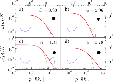
Figure 1: (Color online) Normalized momentum density profiles (MD) for $N=40\textrm{(a)};~{}30\textrm{(b)};~{}10\textrm{(c)};~{}90\textrm{(d)}$ hard-core bosons in a 1d tube, thin (black) lines, at four different sets of parameters are compared to Levy distributions, thick (red) lines. Dashed-doted line (c) corresponds to a Gaussian approximation. The parameters $(N/n_{s},k_{B}T/J)$ are indicated by symbols $\blacklozenge$, $\blacktriangledown$, $\blacksquare$, $\mathbf{\bullet}$ in Fig. 2. The thin solid (blue) icon indicates the confinement geometry.

The momentum distribution can be obtained from the reduced single-particle density matrix $\rho_{n,l}$, reading

$$n(p)=|\Phi(p)|^{2}\sum_{n,l}e^{-ip(n-l)}\rho_{n,l},$$ (2)

where the momentum $p$ is written in units of recoil momentum $\hbar k_{L}=\pi\hbar/d$, and the envelope $\Phi(p)$ is the Fourier transform of the Wannier function. Note that the latter, as well as the hopping $J$, is solely defined by the lattice depth, $V_{0}$, measured in units of recoil energy, $E_{R}=(\hbar k_{L})^{2}/2M$.

To find the reduced single-particle density matrix, we employ here the grand-canonical grandcanon and the canonical formalism canon (See Appendixes A, B). The first is relevant for a system being in contact with a thermal cloud at constant temperature $T$, while the second describes an isolated many-particle system.

The difference between the momentum distributions obtained within the grand-canonical and the canonical descriptions is mediated by the number of particles and becomes negligible for $N\gtrsim 10$ grandcanon . In addition, at finite temperatures $k_{B}T\gtrsim 0.1J$, systems with different number of particles, but the same densities $N/n_{s}$, possess the same momentum profiles grandcanon . Here, $n_{s}=8(J\nu)^{1/2}/\pi$ is the number of single-particle eigenstates with non-zero population at the trap center pendulum . The latter also yields the critical number of bosons in a 1d tube required to form the Mott-insulator in the trap center at zero temperature.

The typical examples of the MD obtained here within the grand-canonical formalism are presented in Fig. 1 for $N\geq 10$, where the results of both the grand-canonical and canonical descriptions practically identical.

III Levy spline approximation

In view of the strong non-Gaussian behavior of the function $n(p)$ (see Fig. 1c) and an apparent power-law intermediate asymptotics bloch ; pollet , it is tempting to compare the MD of a TG gas with symmetric Levy distribution Levy . The latter, $L_{\alpha}(p)$, is a natural generalization of the Gaussian distribution, and it is defined by the Fourier transform of its characteristic function; i.e.,

$$L_{\alpha}(p)=\frac{1}{2\pi}\int_{-\infty}^{\infty}\varphi(\xi)e^{ip\xi}d\xi,~{}~{}~{}\varphi(\xi)=exp(-C_{\alpha}|\xi|^{\alpha})\,,$$ (3)

where the exponent $0<\alpha\leq 2$, and $C_{\alpha}>0$ is some constant Levy . For $\alpha=2$ the distribution is the Gaussian. The value of $\alpha$ is invariant under the scaling transformation $p\rightarrow const\cdot p$, which can be used for fitting.

The Levy distribution exhibits a power-law asymptotics, $L_{\alpha}(p)\propto p^{-(\alpha+1)}$, as $|p|\rightarrow\infty$. These “heavy” tails cause the variance of Levy distributions to diverge for all $\alpha<2$. However, this asymptotic limit is not relevant for our objective: the MD for the system (1) is bounded by the width of $|\Phi(p)|$, $(V_{0}/E_{R})^{1/4}\hbar k_{L}$ pollet , so that the MD variance remains finite.

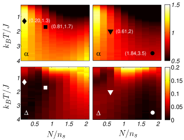
Figure 2: (Color online) The scaling exponent of Levy distribution, $\alpha$ (top), and the corresponding root mean square deviation from the exact momentum density profile, $\Delta$ (bottom), of TG gas as a function of temperature and particle density for two different amplitudes of the optical lattice, $V_{0}=4.6E_{R}$ (left column), and $V_{0}=9.3E_{R}$ (right column), see text for more details. The amplitude of harmonic confinement is chosen as $\nu=2\cdot 10^{-4}E_{R}$.

The fitting of the calculated MD $n(p)$ by the Levy distribution $L_{\alpha}(p)$ was automatized and performed numerically by the global minimum search of the root mean square deviation, $\Delta=\left\{\sum_{n}[n(p_{n})-L_{\alpha}(p_{n})]^{2}\right\}^{1/2}/n(0)$, in a 2d parametric space $\{\alpha,C_{\alpha}\}$ (3). For the results shown on Figs. 1,2, we took $50$ spline points equally spaced on the interval $p\in(0,\hbar k_{L})$. The initial area, ${\alpha\in(0,2),C_{\alpha}\in(0,30)}$, covered by $10\times 10$ grid was iteratively converged to the global minimum by decreasing the grid step in $\alpha$ and $C_{\alpha}$ until the desired relative accuracy (fixed to $1\%$ in all figures) was reached.

In Fig. 2, we show the dependence of scaling exponent $\alpha$ (top) on the scaled temperature $k_{B}T/J$ and the scaled particle density, $N/n_{s}$ (obtained for $N=10,...,100$, and $n_{s}=48.78$), together with the associated mean square deviation $\Delta$ (bottom), at relatively low and high amplitude of the optical lattice. These diagrams (see also Fig. 1, for concrete examples of the MD and their Levy-spline approximations) constitute the first main result of this work, namely, the convergence of the MD of a TG gas towards the Levy distribution with increasing the temperature.

Despite of infinitely strong on-site repulsive interactions, the systematic increase of the Levy exponent $\alpha$ with temperature, cf. Fig. 2 (top), is consistent with the high-temperature limit where the ideal Bose gas obeys the classical Boltzmann-Maxwell statistics with a Gaussian MD, i.e., $\alpha=2$.

IV Averaging over the array of 1d optical lattices

The single 1d tube realization, using a fixed temperature $T$ and a fixed particle number $N$, is not directly accessible with the present state-of-art experiments. The averaging over an array of tubes done in Ref. bloch can be understood as an averaging over many realizations, with different parameters, $T$ and $N$.

Namely, the experimental setup bloch produces an array of independent 1d tubes, with different numbers of particles, $N_{i}$. The probability of having a tube with $N$ particles is given by bloch

$$\varrho(N)=\frac{2}{3}\frac{1}{N^{2/3}_{c}N^{1/3}},~{}~{}N\leq N_{c},$$ (4)

where the number of particles in a central tube $N_{c}$ is a unique parameter. Assuming the same initial temperature in all the tubes for a shallow 1d lattice potential, $V_{\rm in}$, the temperatures at the experimentally adjusted lattice depth, $V_{0}$, can be obtained by using the conservation of entropy in each tube during the subsequent adiabatic increase of the lattice depth from $V_{\rm in}$ to $V_{0}$. Therefore, tubes with the different number of particles, $N_{i}$, acquire different final temperatures, $T_{i}$, at $V_{0}>V_{\rm in}$ bloch .

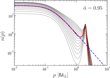
Figure 3: (Color online) Unnormalized momentum distributions (MD) for $N=3,...,18$ hard-core bosons, thin (black) lines, obtained within the canonical approach (11) and the MD averaged over the array of 1d tubes according to the experimental procedure used in Ref. bloch , thick (red) line, with its best Levy-spline, thick (blue) dashed line.

We implemented this averaging procedure with $N_{c}=18$, for a set of individual MDs pre-calculated within the canonical formalism. The result for $k_{B}T=0.5J$, $V_{0}=V_{\rm in}=4.6E_{R}$ and $\nu=8\cdot 10^{-4}E_{R}$ is depicted in Fig. 3.

Surprisingly enough, the averaged MD can be perfectly approximated by the Levy distribution with an “average” scaling exponent, $\tilde{\alpha}$; this is so despite the sizable dispersion of $\alpha$-values appearing in the different momentum profiles.

Therefore, the averaged momentum profile appears as a superposition of several different profiles. It is known that using a proper weight function, $f(\beta)$, one can construct a Levy distribution from a parameterized set of Gaussian distributions of different dispersion, $L_{\alpha}(p)=\int_{-\infty}^{\infty}G(p,\beta)f(\beta)d\beta$ superstat . Yet, to the best of our knowledge, there are no results concerning the superposition of many different Levy distribution functions with different exponents $\alpha$.

A next objective is the comparison of our scheme with the experimental data from Ref. bloch , see Fig. 4. As one can deduce the Levy distribution yields an excellent approximation for the MD of the experimental system although the latter does not map precisely to a TG gas, but rather corresponds to a set of $N$ soft-core bosons with $U/J<\infty$ (1) pollet . In the experiment, one used a power-law fit, $n(p)\propto p^{-\gamma_{exp}}$, on an intermediate range ($0.3\leq|p/\hbar k_{L}|\leq 1$) bloch , with $\gamma_{\rm exp}-1=1.2;~{}0.9;~{}0.4;~{}0.2$ for the data shown on Figs. 4(a-d), respectively. We emphasize, however, that in the experimentally accessible region, $|p|\lesssim\hbar k_{L}$, the power law behavior with the exponent $\gamma_{\rm exp}-1=\tilde{\alpha}$ of the Levy distribution is not yet valid, but is assumed only for much larger momentum values. Therefore, the theoretical estimates $\tilde{\alpha}$ in Fig. 4 exceed those intermediate range power-law fit-values, i.e. one consistently finds that $\tilde{\alpha}>\gamma_{\rm exp}-1$.

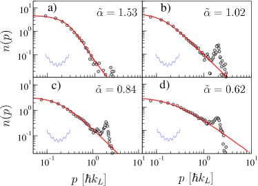
Figure 4: (Color online) The experimental data for the MD of the 1d quantum gases for different axial lattice depths bloch , grey dots; Levy distributions with the scaling exponent $\tilde{\alpha}$, solid (red) lines. The thin solid (blue) icon indicates the confinement geometry.

V Universality of the Levy-spline for a Tonks-Girardeau gas in 1d confinement potentials

So far we have been dealing with a TG gas on a lattice with an additional harmonic potential (1), which is the only confinement where the MD of a TG gas was experimentally studied in detail bloch . In the present section, we demonstrate applicability of the Levy-spline approximation to the numerically obtained MD of hard-core bosons at finite temperatures in various 1d confinements: a sole harmonic trap, Fig. 5, a box, Fig. 6(a,b), and a sole optical lattice with impenetrable boundaries, Fig. 6(c,d).

A TG gas confined in a general potential, $V(x)$, is described by the sum of the single particle Hamiltonians,

$$H=\sum_{i=1}^{N}\left(-\frac{\hbar^{2}}{2M}\frac{\partial^{2}}{\partial x_{i}^{2}}+V(x_{i})\right)$$ (5)

with the hard-core constrain on the bosonic many-particle wave function: $\Psi(x_{1},x_{2},...,x_{N})=0$ if $|x_{i}-x_{j}|<a$, where $x_{i}$ is the position of $i$th particle, and $a$ is the 1d hard-core diameter. At low density, hard-bosons can be approximated by impenetrable point size particles, so that $a=0$ tonk .

The MD of $N$ hard-bosons in a box, $V_{\rm box}(x_{i})=0$ if $0<x_{i}<L_{\rm box}$ and $V_{\rm box}=\infty$ otherwise, and in a harmonic confinement, $V_{\rm osc}=m\omega^{2}x_{i}^{2}/2$, was obtained numerically within the canonical formalism with the help of efficient method buljan , which is detailed in Appendix B.2. In the case of a sole lattice potential with $L$ lattice sites, the MD was calculated within the grand-canonical formalism by using the same algorithm that was employed in Sec. IV (see Appendix A).

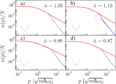
Figure 5: (Color online) Normalized momentum density profiles (MD) for $N=5\textrm{(a,b)};~{}10\textrm{(c,d)}$ hard-core bosons in a sole 1d harmonic trap, thin (black) lines, at the two different temperatures, $k_{B}T/\hbar\omega_{0}=1$ (a,c), $k_{B}T/\hbar\omega_{0}=1.5$ (b,d) are compared to Levy distributions, thick (red) lines. Dashed line (c) underlines well known universal power-law asymptotic behavior of the Tonks-Girardeau gas momentum distribution at large momenta, $p^{-4}$, while dashed-dotted line illustrates failure of a Gaussian approximation. The thin solid (blue) icon indicates the confinement geometry.

It is known, that the MD of a TG gas in a homogeneous toroidal trap and in a harmonic confinement (Fig. 5) exhibits a power-law behavior, $p^{-4}$, for $p\rightarrow\infty$ olshani . We also found the same power-law behavior for a TG gas in a box, see Fig. 6(a,b). This in fact turns out to be a general feature of a TG, which also persists at finite temperatures. However, the power-law tail, $p^{-\alpha-1}$, of the Levy distribution with exponent $\alpha$ cannot decay faster than $p^{-3}$ Levy . Therefore, our Levy-spline approximation is exclusively aimed to a finite momentum region $(0,p_{\rm c})$, where the asymptotic $p^{-4}$ behavior has not yet developed. With Figs. 5-6, we demonstrate that the MD of a TG gas at finite temperatures in various 1d confinement potentials (thin lines) can be perfectly approximated by Levy-splines (thick lines) over significant momentum range.

While at zero temperature we detect a notable deviation of the Levy-spline from the actual MD, with increasing the temperature the deviation becomes practically negligible. The exponent of Levy-splines for a TG gas in the confinement potentials presented here depends, in general, on the confinement characteristics, on the gas temperature and on the particle number or the filling factor, $N/L$ (in the case of a lattice). A more detailed analysis of this dependence will be addressed elsewhere.

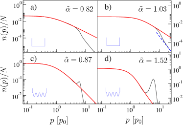
Figure 6: (Color online) Normalized momentum density profiles (MD) for $N=10\textrm{(a,d)};~{}5\textrm{(b)};~{}50\textrm{(c)}$ hard-core bosons in a 1d box (a,b) of size $L_{\rm box}$ and on a lattice (c,d) with $L=100$ lattice sites and the potential amplitudes $V_{0}=4.6E_{R}\textrm{(c)};~{}9.9E_{R}\textrm{(d)}$, thin (black) lines, at the temperatures $k_{B}T/\hbar\omega_{\rm box}=20$ (a); $10$ (b), $k_{B}T/J=0.5$ (c,d) are compared to Levy distributions, thick (red) lines. Here the frequency $\omega_{\rm box}=\hbar\pi^{2}/2ML_{\rm box}$ sets the energy scale, $\hbar\omega_{0}$, for a particle in a box. The momentum, $p$, is measured in units of $p_{0}=\hbar/L_{\rm box}$(a,b) and $p_{0}=\hbar k_{L}$ (c,d), in the case of a lattice potential and a box, respectively. The thin solid (blue) icons indicate the two corresponding types of confinement geometry.

VI Conclusions

We have presented a study of the finite-temperature momentum distribution (MD) of Tonks-Girardeau (TG) gases confined in various 1d confinement potentials. The MD of a TG gas on an optical lattice with a superimposed harmonic confinement depends on the particle density, on the lattice depth and on the gas temperature. We have shown that the tunable Levy distribution fits momentum profiles up to one recoil momentum with high accuracy. This allows for calibration of TG states with a unique scaling exponent. Thus, our approach completes the attempts to quantify the finite-temperature MDs by using a power-law fitting for the intermediate region $0.3\leq|p/\hbar k_{L}|\leq 1$ bloch ; pollet .

We demonstrate that the MD of a TG gas confined in a 1d box, in a sole 1d harmonic potential and on a 1d optical lattice with hard wall boundaries can be approximated by the Levy distribution function (3) on a finite momentum region $(0,p_{\rm c})$, where for a TG gas the universal power-law, $p^{-4}$, at large momenta has not yet developed. We thus conjecture that Levy scaling of MD is generic feature of a thermalized TG gas.

We want to emphasize one aspect which we consider to be crucial for the understanding of our approach. It is known that the Levy distribution has appeared as the stable distribution, i.e. the “attractor” for normalized sums of independent and identically-distributed random variables, with no finite mean values. The latter has opened the door to anomalous statistics Levy . In our approach, we employ the Levy distribution (3) merely as a mathematical function, which is a natural generalization of the standard Gaussian function, thus leaving aside all the possible statistical interpretations and speculations concerning physical processes responsible for the MD formation. A good example for such “applied” approaches is the widespread use of the Gaussian distribution, which describes the wave function of the ground state of the quantum harmonic oscillator Liboff , the Green’s function solution of the deterministic heat or diffusion equation heat , and frequently results as a form function in many different physical contexts.

While it is intuitively clear that it is the long-range correlations in the system that cause the emergence of Levy distributions, the task to unravel the inherent physical mechanism(s) yielding this anomalous distribution remains a challenge. We think that the analysis of a reduced single-particle density matrix in a spirit of the theory of random Levy matrices Levy_matrix may shed additional light on this intriguing issue.

Appendix A Grand-canonical formalism

Within the grand-canonical description, the number of bosons, $N$, is a fluctuating quantity and the reduced single-particle density matrix is defined as the trace over the Fock space,

$$\rho_{n,l}=\frac{1}{Z}\textrm{Tr}\left\{\langle b_{n}^{\dagger}b_{l}\rangle e^{-\beta(H-\mu\sum_{j}n_{j})}\right\},$$ (6)

where the chemical potential $\mu$ is fixed to give the required number of particles $N=\sum_{l}\rho_{l,l}$ in the system, $\beta=1/k_{B}T$ with $k_{B}$ being the Boltzmann factor, and $Z$ is the grand-canonical partition function. The latter coincides with that of non-interacting fermions, i.e., $Z=\prod_{j}[1+e^{-\beta(\epsilon_{j}-\mu)}]$, where $\epsilon_{j}$ stands for the single-particle energy spectrum.

The trace over the the Fock space (6) can be evaluated exactly grandcanon by mapping the problem of hard-core bosons on that of spinless fermions via the Jordan-Wigner transformation jordanwigner . We next use the expressions for the elements of the reduced single-particle density matrix elaborated in grandcanon , i.e.,

$$\rho_{n,l}=\frac{1}{Z} \left\{\det\left[\mathbf{I}+(\mathbf{I}+\mathbf{A}(n,l))\mathbf{D}(n,l)\right]\right.$$ (7)

$$\left.-\det\left[\mathbf{I}+\mathbf{D}(n,l)\right]\right\}\,,\mbox{for}\,n\neq l,$$

$$\mathbf{D}(n,l)=\mathbf{O}(l)\mathbf{U}e^{-(\mathbf{E}-\mu\mathbf{I})/k_{B}T}\mathbf{U}^{\dagger}\mathbf{O}(n);$$ (8)

and

$$\rho_{n,n}=\left[\mathbf{U}\left(\mathbf{I}+e^{(\mathbf{E}-\mu\mathbf{I})/k_{B}T}\right)^{-1}\mathbf{U}^{\dagger}\right]_{n,n},$$ (9)

for the main diagonal elements. All operators entering above are the square matrices $N\times N$ defined as follows: $\mathbf{I}$ denotes the identity matrix, $\mathbf{O}(n)_{i,j}=\{-\delta_{i,j},i\leq n-1;\delta_{i,j},i>n-1\}$, $\mathbf{A}(n,l)_{i,j}=\delta_{i,n}\delta_{j,l}$, $\mathbf{U}$ is the orthogonal matrix of eigenvectors satisfying the eigenproblem, $H_{1}\mathbf{U}=\mathbf{U}\mathbf{E}$, with single-particle version of Hamiltonian (1)

$$H_{1}=-J\sum_{l}(|l+1\rangle\langle l|+h.c.)+\nu\sum_{l}l^{2}|l\rangle\langle l|,$$ (10)

and $\mathbf{E}$ is diagonal matrix of its eigenvalues, i.e., $\mathbf{E}_{i,j}=\varepsilon_{i}\delta_{i,j}$. Thus, to obtain the entire matrix $\rho_{n,l}$ ($\rho_{l,n}=\rho_{n,l}^{*}$) one has to compute $N(N-1)/2$ determinants of $N\times N$ matrices.

Appendix B Canonical formalism

In the canonical formalism, the particle reservoir is absent, meaning that one has to find the number, $\mathcal{N}_{e}$, self-consistently from those many particle states, $|\Psi^{m}\rangle$, together with their eigenenergies, $E_{m}$, that contribute to the thermal superposition at a given temperature. The reduced single-particle density matrix is then obtained as a sum of thermally weighted density matrices, $\rho^{m}$, evaluated for each from $\mathcal{N}_{e}$ eigenstates separately; i.e.,

$$\rho=\frac{1}{\mathcal{Z}}\sum_{m=1}^{\mathcal{N}_{e}}e^{-\beta E_{m}}\rho^{m}.$$ (11)

The canonical partition function $\mathcal{Z}$ is expressed through the true many particle energy spectrum: $\mathcal{Z}=\sum_{m=1}^{\mathcal{N}_{e}}e^{-\beta E_{m}}$.

The energy spectrum of hard-core bosons is the same as that for spinless fermions: $E_{m}=\sum_{n=1}^{N}\epsilon_{\alpha_{n}^{m}}$, where $\alpha_{n}^{m}$ denotes the numbers of single-particle eigenlevels occupied in the $m$-th many-particle state.

B.1 Hard-core bosons on a lattice

In the case of a lattice confinement, $\rho^{m}\equiv\rho_{n,l}^{m}=\langle\Psi^{m}|b_{n}^{\dagger}b_{l}|\Psi^{m}\rangle$. The corresponding many-particle eigenstates can be represented as

$$|\Psi^{m}\rangle=\prod_{\alpha_{n}^{m}}\sum_{l}\mathbf{U}_{l,\alpha_{n}^{m}}b_{l}^{\dagger}|0\rangle,\,n=1,\dots,N$$ (12)

where $\mathbf{U}$ is complete orthogonal set of single-particle eigenvectors (see Appendix A).

Each contribution, $\rho_{i,j}^{m}$, is related to the Green function, $G_{i,j}^{m}=\langle\Psi^{m}|b_{i}b_{j}^{\dagger}|\Psi^{m}\rangle$:

$$\rho_{i,j}^{m}=G_{i,j}^{m}+\delta_{i,j}(1-2G_{i,j}^{m}).$$ (13)

Using the Jordan-Wigner transformation jordanwigner , the bosonic Green function can be rewritten as scaler product of two fermionic wave-functions, and subsequently as a determinant of matrix product canon :

$$G_{i,j}^{m}={\rm det}\left[(\mathbf{P}_{m}(i))^{\dagger}\mathbf{P}_{m}(j)\right],$$ (14)

where the matrix $\mathbf{P}_{m}(i)_{l,n}$ has $N+1$ columns

$$\mathbf{P}_{m}(i)_{l,n}=\left\{\begin{array}[]{cl}-\mathbf{U}_{l,\alpha_{n}^{m}},&\mbox{for}\,l\leqslant i-1,n=1,\dots,N;\\ \mathbf{U}_{l,\alpha_{n}^{m}},&\mbox{for}\,l>i-1,n=1,\dots,N;\\ \delta_{i,l},&\mbox{for}\,n=N+1.\\ \end{array}\right.$$ (15)

In comparison to the grand-canonical approach, the number of operations needed to obtain the entire matrix $\rho_{i,j}$ is a factor of $\mathcal{N}_{e}$ larger, and is growing with increasing temperature.

B.2 Hard-core bosons in arbitrary confinement potential

Above we detailed the canonical formalism for hard-core bosons on a lattice. Here, instead, we elaborate on a general case with arbitrary confinement, $V(x)$. In this case, the momentum distribution, $n(p)$, can be obtained from the reduced single-particle density matrix in the continuum: $n(p)=(2\pi)^{-1}\int dxdye^{-ik(x-y)}\rho(x,y)$, where $\rho(x,y)$ is given by the thermal superposition (11) with $\rho^{m}\equiv\rho^{m}(x,y)$ defined below.

To calculate the reduced single-particle density matrix, $\rho^{m}(x,y)$, in the continuum we make use of efficient method buljan , which represents it in terms of the single particle states:

$$\rho^{m}(x,y)=\sum_{i,j=1}^{N}\psi_{\alpha_{i}^{m}}^{*}(x)A^{m}(x,y)_{i,j}\psi_{\alpha_{j}^{m}}(y),\\$$ (16)

where $N\times N$ matrix $\mathbf{A}^{m}(x,y)$ associated to the $m$-th many-particle state is

$$A^{m}(x,y)_{i,j}=\left(-1\right)^{i+j}\det\mathbf{Q}_{m}(i,j).$$ (17)

$\mathbf{Q}_{m}(i,j)$ is a minor of matrix $\mathbf{Q}_{m}$ obtained by crossing $i$-th row and $j$-th column, and matrix $\mathbf{Q}_{m}$ itself is given as

$$Q_{m}(x,y)_{i,j}=\delta_{i,j}-2\int_{x}^{y}dx^{\prime}\psi_{\alpha_{i}^{m}}^{*}(x^{\prime})\psi_{\alpha_{j}^{m}}(x^{\prime}),$$ (18)

where $\psi_{n}(x)$ are the eigenfunctions of single particle eigenproblem in a given trapping potential $V(x)$. In (18), it is assumed that $x\geq y$, while for $x\leq y$: $\rho^{m}(x,y)=\rho^{m}(y,x)^{*}$. The set of $\alpha_{i}^{m}$, as before in Appendix B.1, denotes the numbers of single-particle eigenlevels occupied in the $m$-th many-particle state. Additionally, whenever $\det\mathbf{Q}_{m}\neq 0$, (17) can be represented as $\mathbf{A}^{m}=\left(\mathbf{Q}_{m}^{-1}\right)^{T}\det{\mathbf{Q}_{m}}$ buljan , which is more efficient when implemented numerically.

For a box and for a harmonic confinement, $\psi_{n}(x)=\sqrt{2/L_{\rm box}}\sin(n\pi x/L_{\rm box})$ and $\psi_{n}(x)=\sqrt{1/2^{n}n!}\left(m\omega_{0}/\pi\hbar\right)^{1/4}\exp\left(-m\omega_{0}x^{2}/2\hbar\right)H_{n}(\sqrt{m\omega_{0}/\hbar}x)$, respectively, where $H_{n}(y)$ are the Hermite polynomials. For these confinements, the integral in (18), and the density matrices $\rho^{m}(x,y)$ can be obtained analytically for a small number of particles with the help of symbolic computational routines. However, expanding out $m$ times $N^{2}$ determinants of $(N-1)\times(N-1)$ matrices for $N\gtrsim 5$ quickly becomes unwieldy. Therefore, in Sec. V, the reduced density matrices $\rho^{m}(x,y)$ were calculated on a numerical grid. The grid step was sufficiently small to ensure a smooth representation of all single particle wave-functions, $\psi_{m}(x)$, participating in excited many-particle states at a given temperature.

References

- (1) D. J. Thouless, The Quantum Mechanics of Many-body Systems (Academic Press, New York, 1972); A. L. Fetter and J. D. Walecka, Quantum Theory of Many-Particle Systems (Dover, New York, 2003).
- (2) H. J. Metcalf and P. van der Straten, Laser Cooling and Trapping (Springer, New York, 1999).
- (3) O. Morsch and M. Oberthaler, Rev. Mod. Phys. 78, 179 (2006).
- (4) I. Bloch, J. Dalibard, and W. Zwerger, Rev. Mod. Phys. 80, 885 (2008).
- (5) M. Girardeau, J. Math. Phys. 1, 516 (1960).
- (6) B. Paredes et al., Nature 429, 277 (2004).
- (7) T. Kinoshita, T. Wenger, and D. S. Weiss, Science 305, 1125 (2004).
- (8) M. Olshanii and V. Dunjko, Phys. Rev. Lett. 91, 090401 (2003).
- (9) T. Papenbrock, Phys. Rev. A 67, 041601(R) (2003).
- (10) A. Minguzzi, P. Vignolo, and M. P. Tosi, Phys. Lett. A 294, 222 (2002).
- (11) L. Pollet, S. M. A. Rombouts, and P. J. H. Denteneer, Phys. Rev. Lett. 93, 210401 (2004).
- (12) W. Feller, An Introduction to Probability Theory and Its Applications (John Wiley and Sons, New York, 1970), Vol.2.
- (13) M. F. Shlesinger, G. M. Zaslavsky, and J. Klafter, Nature 363, 31 (1993); A. Blumen, G. Zumofen, and J. Klafter, Phys. Rev. A 40, 3964 (1989).
- (14) F. Bardou, J.-P. Bouchaud, A. Aspect and C. Cohen-Tannoudji, Levy Statistics and Laser Cooling (Cambridge Univ. Press, Cambridge 2000).
- (15) R. N. Mantegna and H. E. Stanley, Nature 376, 46 (1995).
- (16) E. Barkai, R. Silbey, and G. Zumofen, Phys. Rev. Lett. 84, 5339 (2000).
- (17) R. Segev et al., Phys. Rev. Lett. 88, 118102 (2002).
- (18) C.-K. Peng et al., Phys. Rev. Lett. 70, 1343 (1993).
- (19) M. Rigol, Phys. Rev. A 72, 063607 (2005).
- (20) M. Rigol and A. Muramatsu, Phys. Rev. A 70, 031603(R) (2004); ibid., 72, 013604 (2005).
- (21) D. Jaksch, C. Bruder, J. I. Cirac, C. W. Gardiner, and P. Zoller, Phys. Rev. Lett. 81, 3108 (1998).
- (22) The critical density is found via mapping the single particle version of (1) onto the quantum pendulum avp .
- (23) A. V. Ponomarev and A. R. Kolovsky, Laser Phys. 16, 367 (2006).
- (24) C. Beck and E. G. D. Cohen, Physica A 322, 267 (2003).
- (25) R. Pezer and H. Buljan, Phys. Rev. Lett. 98, 240403 (2007).
- (26) R. L. Liboff, Introductory Quantum Mechanics (Addison-Wesley, London, 2002).
- (27) G. Barton, Elements of Green’s functions and Propagation (Clarendon press, Oxford, 1989).
- (28) P. Cizeau and J. P. Bouchaud, Phys. Rev. E 50, 1810 (1994).
- (29) P. Jordan and E. Wigner, Z. Phys. 47, 631 (1928).