Lindelöf’s theorem for catenoids revisited

Abstract

In this paper we study the maximal stable domains on minimal catenoids in Euclidean and hyperbolic spaces and in $\mathbb{H}^{2}\times\mathbb{R}$. We in particular investigate whether half-vertical catenoids are maximal stable domains (Lindelöf’s property). We also consider stable domains on catenoid-cousins in hyperbolic space. Our motivations come from Lindelöf’s 1870 paper on catenoids in Euclidean space.

Mathematics Subject Classification (2000):  53C42, 53C21, 58C40

Key words:  Minimal surfaces. Constant mean curvature surfaces. Stability. Index.

1 Introduction

In his 1870 paper “Sur les limites entre lesquelles le caténoïde est une surface minima” published in the second volume of the Mathematische Annalen, see [8], L. Lindelöf determines which domains of revolution on the catenoid ${\mathcal{C}}$ in $\mathbb{R}^{3}$ are stable. More precisely, he gives the following geometric construction (see Figure 1).

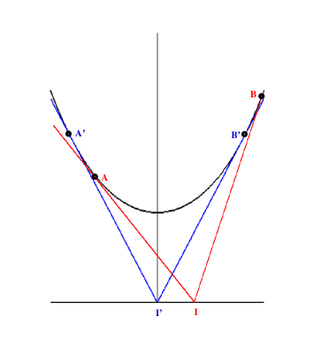
Figure 1: Lindelöf’s construction

Take any point $A$ on the generating catenary $C=\{(x,z)\in\mathbb{R}^{2}\leavevmode\nobreak\ |\leavevmode\nobreak\ z=\cosh(x)\}$. Draw the tangent to $C$ at the point $A$ and let $I$ be the intersection point of the tangent with the axis $\{z=0\}$. From $I$, draw the second tangent to $C$. It touches $C$ at the point $B$. Lindelöf’s result states that the compact connected arc $AB$ generates a maximal weakly stable domain on the catenoid ${\mathcal{C}}$ in the sense that the second variation of the area functional for this domain is zero while it is positive for any smaller domain, and negative for any larger domain.

As a consequence, the upper-half of the catenoid, ${\mathcal{C}}\cap\{x\geq 0\}$ is a maximal weakly stable among domains invariant under rotations. We will refer to this latter property as Lindelöf’s property.

In this paper, we generalize Lindelöf’s result (not the geometric construction with tangents), to other catenoid-like surfaces: catenoids in $\mathbb{H}^{3}$ and $\mathbb{H}^{2}\times\mathbb{R}$, embedded catenoid-cousins (rotation surfaces with constant mean curvature $1$ in $\mathbb{H}^{3}(-1)$).

The global picture looks as follows. Catenoids in $\mathbb{R}^{3}$ and catenoid-cousins in $\mathbb{H}^{3}$ satisfy Lindelöf’s property. That minimal catenoids in $\mathbb{R}^{3}$ and catenoid-cousins in $\mathbb{H}^{3}$ have similar properties is not surprising from the local correspondence between minimal surfaces in $\mathbb{R}^{3}$ and surfaces with constant mean curvature $1$ in $\mathbb{H}^{3}(-1)$. One may observe that the Jacobi operators look the same, namely $-\Delta-|A_{0}|^{2}$, where $A_{0}$ is the second fundamental form for catenoids and its traceless analog for catenoid-cousins.

Catenoids in $\mathbb{H}^{2}\times\mathbb{R}$ have index $1$ and do not satisfy Lindelöf’s property. Catenoids in $\mathbb{H}^{3}$ divide into two families, a family of stable catenoids which foliate the space, and a family of index $1$ catenoids which intersect each other and have an envelope. The hyperbolic catenoids do not satisfy Lindelöf’s property. One may observe that the Jacobi operators can be written $-\Delta+c-|A|^{2}$, where $c=1$ for catenoids in $\mathbb{H}^{2}\times\mathbb{R}$ and $c=2$ for catenoids in $\mathbb{H}^{3}$. The presence of $c$ may explain the extra stability properties of these catenoids.

To prove his result, Lindelöf introduced the $1$-parameter family of Euclidean catenoids passing through a given point and considered the Jacobi field associated with the variation of this family. In this paper we work directly with Jacobi fields. More precisely, we consider the vertical Jacobi field (associated with the translations along the rotation axis in the ambient space), the variation Jacobi field (the catenoids come naturally in a $1$-parameter family) and a linear combination of these two Jacobi fields which is well-suited to study Lindelöf’s property.

In some instances, we could use alternative methods to prove (or disprove) Lindelöf’s property. For example, the fact that Euclidean catenoids satisfy Lindelöf’s property follows from the theorem of Barbosa - do Carmo, see [1], relating the stability of a domain with the area of its spherical image by the Gauss map. One could also use the fact that the Jacobi operator on the Euclidean catenoid is transformed into the operator $-\Delta-2$ on the sphere minus two points by a conformal map.

Such alternative methods are not always available. On the other-hand, our method applies to catenoids in higher dimensions as well as to rotation surfaces with constant mean curvature $H$, $0\leq H\leq 1$ in the hyperbolic space $\mathbb{H}^{3}(-1)$. These catenoids or catenoid-like hypersurfaces do not satisfy Lindelöf’s property.

We finally point out that among the examples we have studied, the hypersurfaces which do not satisfy Lindelöf’s property are precisely those which are vertically bounded.

Note that the stability of (minimal) catenoids have been studied in [4, 9, 12] when the ambient space is $\mathbb{H}^{3}$, in [3, 10] when the ambient space is $\mathbb{H}^{2}\times\mathbb{R}$ and that the index of catenoid-cousins has been studied in [7].

The paper is organized as follows. In Section 2, we recall some basic notations and facts. We review Lindelöf’s original result in Section 3. In Section 4, we study Lindelöf’s result for $n$-catenoids (minimal rotation hypersurfaces) in Euclidean space $\mathbb{R}^{n+1}$. In Sections 5 and 6, we consider catenoids in $\mathbb{H}^{2}\times\mathbb{R}$ and $\mathbb{H}^{n}\times\mathbb{R}$. In Section 7, we study minimal catenoids and catenoid-cousins in $\mathbb{H}^{3}$.

The authors would like to thank Manfredo do Carmo for pointing out Lindelöf’s paper to them.

The authors would like to thank the Mathematics Department of PUC-Rio (PB) and the Institut Fourier – Université Joseph Fourier (RSA) for their hospitality. They gratefully acknowledge the financial support of CNPq, FAPERJ, Université Joseph Fourier and Région Rhône-Alpes.

2 Preliminaries

Let $(\widehat{M},\widehat{g})$ be an orientable Riemannian manifold and let $M^{n}\looparrowright\widehat{M}^{n+1}$ be a complete orientable minimal immersion. The second variation of the area functional is given by the Jacobi operator $J_{M}$ acting on $C^{\infty}_{0}(M)$,

(2.1) $$J_{M}=-\Delta-\big{(}\widehat{\mathrm{Ric}}(N,N)+|A|^{2}\big{)},$$

where $\Delta$ is the (non-positive) Laplacian in the induced metric on $M$, $N$ a unit normal field along the immersion, $A$ the second fundamental form of the immersion with respect to $N$ and $\widehat{\mathrm{Ric}}$ the Ricci curvature of the ambient space $\widehat{M}$, see [6].

The Jacobi operator appears naturally when one considers families of constant mean curvature immersions. More precisely, let $X(a,\cdot):M^{n}\looparrowright(\widehat{M}^{n+1},\widehat{g})$ be a $1$-parameter family of orientable immersions with unit normal $N(a,x)$ and constant mean curvature $H(a)$. Let $u(a,x):=\widehat{g}(\frac{\partial X}{\partial a}(a,x),N(a,x))$. Then, see [2],

(2.2) $$H^{\prime}(a)=\Delta u+\big{(}\widehat{\mathrm{Ric}}(N,N)+|A|^{2}\big{)}u=-J_{M}(u).$$

In particular, if $H(a)$ does not depend on $a$, then $u$ satisfies the equation $J_{M}(u)=0$.

We call Jacobi field on $D\subset M$ a $C^{\infty}$ function $f$ such that $J_{M}(f)=0$ on $D$. The geometry of the ambient space provides usefull Jacobi fields. More precisely, the following classical properties follows immediately from Equation (2.2).

Property 2.1 (Killing Jacobi field)

Let $M\looparrowright\widehat{M}$ be a minimal or constant mean curvature immersion and let ${\mathcal{K}}$ be a Killing field on $\widehat{M}$. The function $f_{{\mathcal{K}}}=\widehat{g}({\mathcal{K}},N)$, given by the inner product (in $\widehat{M}$) of the Killing field ${\mathcal{K}}$ with the unit normal $N$ to the immersion, is a Jacobi field on $M$.

Property 2.2 (Variation Jacobi field)

Let $X(a,\cdot):M\looparrowright\widehat{M}$ be a smooth family of immersions, with the same constant mean curvature $H$, for $a$ in some interval around $a_{0}$. Then the function $v=\widehat{g}(\frac{\partial X}{\partial a}(a_{0},\cdot),N)$, the scalar product of the variation vector field of the family with the unit normal $N$ to the immersion $X(a_{0},\cdot)$, is a Jacobi field on $X(a_{0},M)$.

We say that a domain $D$ on $M$ is stable if $\int_{M}fJ_{M}(f)\,d\mu_{M}>0$ for all $f\in C^{\infty}_{0}(D)$, where $d\mu_{M}$ is the Riemannian measure for the induced metric on $M$. We say that a domain $D$ on $M$ is weakly stable if $\int_{M}fJ_{M}(f)\,d\mu_{M}\geq 0$ for all $f\in C^{\infty}_{0}(D)$. We say that a relatively compact open domain $D$ on $M$ has index $k$ if the maximal dimension of subspaces of $C^{\infty}_{0}(D)$ on which $\int_{D}fJ_{M}(f)\,d\mu_{M}$ is negative, is equal to $k$. Finally, we say that an open domain is maximally weakly stable if it is weakly stable and if any bigger open domain is not.

Let $D\subset M$ be a relatively compact regular open domain, and let

$$\lambda_{1}(D)=\inf\{\int_{D}fJ_{M}(f)\,d\mu_{M}\leavevmode\nobreak\ |\leavevmode\nobreak\ f\in C^{\infty}_{0}(D),\int_{M}f^{2}\,d\mu_{M}=1\},$$

be the least eigenvalue of the Jacobi operator $J_{M}$ with Dirichlet boundary conditions on $\partial D$. To say that $D$ is weakly stable but not stable is equivalent to saying that $\lambda_{1}(D)=0$.

Property 2.3 (Monotonicity)

Let $D_{1}\subset D_{2}$ be two relatively compact domains in $M$, such that $\mathrm{int}(D_{2}\setminus D_{1})\not=\emptyset$. Then $\lambda_{1}(D_{1})>\lambda_{1}(D_{2})$. In particular, if $D_{2}$ is weakly stable (i.e. $\lambda_{1}(D_{2})\geq 0$) and $\mathrm{int}(D_{2}\setminus D_{1})\not=\emptyset$, then $D_{1}$ is stable (i.e. $\lambda_{1}(D_{1})>0$).

Property 2.4 (Stability criterion)

A relatively compact domain $D$ is weakly stable if and only if there exists a positive function $u:D\to\mathbb{R}_{+}$ such that $J_{M}(u)\geq 0$.

Property 2.3 is the classical monotonicity principle of Dirichlet eigenvalues. Property 2.4 follows from the divergence theorem.

$\blacktriangleright$ [PB2]

[PB2] $\blacktriangleleft$

3 Catenoids in $\mathbb{R}^{3}$

We consider the family of catenoids given by the following parametrization

(3.3) $$X(a,t,\theta)=\big{(}a\cosh(\frac{t}{a})\cos\theta,a\cosh(\frac{t}{a})\sin\theta,t\big{)},\leavevmode\nobreak\ a>0$$

and in particular the catenoid ${\mathcal{C}}$ given by $X_{1}$. The unit normal to ${\mathcal{C}}_{a}$ is

(3.4) $$N(a,t,\theta)=\big{(}-\dfrac{\cos\theta}{\cosh(\frac{t}{a})},-\dfrac{\sin\theta}{\cosh(\frac{t}{a})},\tanh(\frac{t}{a})\big{)}.$$

$\blacktriangleright$ [PB2]

[PB2] $\blacktriangleleft$

The Jacobi operator on ${\mathcal{C}}$ is

(3.5) $$J_{{\mathcal{C}}}=-\cosh^{-2}(t)\big{(}\dfrac{\partial^{2}}{\partial t^{2}}+\dfrac{\partial^{2}}{\partial\theta^{2}}\big{)}-2\cosh^{-4}(t),$$

with radial part

(3.6) $$J_{{\mathcal{C}}}^{0}=-\cosh^{-2}(t)\dfrac{\partial^{2}}{\partial t^{2}}-2\cosh^{-4}(t)=\cosh^{-2}(t)L_{{\mathcal{C}}}.$$

According to Property 2.1, the function

(3.7) $$v(t)=\tanh(t)=\langle\frac{\partial}{\partial z},N(t,\theta)\rangle$$

is a Jacobi field on ${\mathcal{C}}$. According to Property 2.2, the function

(3.8) $$e(t)=1-t\,\tanh(t)=-\langle\frac{d}{da}X_{a}|_{a=1}(a,t,\theta),N(t,\theta)\rangle$$

is a Jacobi field on ${\mathcal{C}}$.

$\blacktriangleright$ [PB2]

[PB2] $\blacktriangleleft$

Theorem 3.1

Let $\xi_{0}$ be the positive zero of the function $e(t)=1-t\,\tanh(t)$.

1. The domain ${\mathcal{D}}_{\xi_{0}}=X(1,]-\xi_{0},\xi_{0}[,[0,2\pi])$ is a maximal weakly stable domain on the catenoid ${\mathcal{C}}$.

2. The domain ${\mathcal{D}}_{+}=X(1,]0,\infty[,[0,2\pi])$ is a maximal weakly stable rotation invariant domain on the catenoid ${\mathcal{C}}$. More precisely, given any $\alpha>0$, the function

   (3.9) $$e(\alpha,t)=v(\alpha)e(t)+e(\alpha)v(t).$$

   has a unique positive zero $\beta(\alpha)$ and the domain ${\mathcal{D}}_{\alpha,\beta(\alpha)}=X(1,]-\alpha,\beta(\alpha)[,[0,2\pi])$, is a maximal weakly stable rotation invariant domain in ${\mathcal{C}}$.

3. The catenoid ${\mathcal{C}}$ has index $1$.

Proof of Theorem 3.1.

1.  The function $e(t)$ is a Jacobi field on ${\mathcal{C}}$ which satisfies

$$\left\{\begin{array}[]{ll}J_{{\mathcal{C}}}(e)&=0\text{\leavevmode\nobreak\ in\leavevmode\nobreak\ }{\mathcal{D}}_{\xi_{0}},\\ e|{\partial{\mathcal{D}}_{\xi_{0}}}&=0.\\ \end{array}\right.$$

It follows that $\lambda_{1}({\mathcal{D}}_{\xi_{0}})=0$ and hence, any smaller open domain $\Omega\varsubsetneq{\mathcal{D}}_{\xi_{0}}$ is stable, while any larger open domain ${\mathcal{D}}_{\xi_{0}}\varsubsetneq\Omega$ is unstable by Property 2.3.

2.  The function $v(t)$ being positive in the interior of ${\mathcal{D}}_{+}$, it follows from Property 2.4 that ${\mathcal{D}}_{+}$ is weakly stable. Take any $\alpha>0$. Because $e$ and $v$ are Jacobi fields, the function $e(\alpha,t)$ defined by (3.9) is a Jacobi field too and satisfies $e(\alpha,-\alpha)=0$. Because $e(\alpha,\pm\infty)=-\infty$ and $\frac{\partial e}{\partial t}(\alpha,-\alpha)\not=0$, the function $e(\alpha,\cdot)$ must have another zero $\beta(\alpha)\not=-\alpha$. That this second zero is unique and positive can be seen directly, or arguing as follows. First of all, observe that the function $e(\alpha,\cdot)$ cannot have two negative zeroes or two positive zeroes because ${\mathcal{D}}_{-}=X(1,]-\infty,0[,[0,2\pi])$ and ${\mathcal{D}}_{+}$ are weakly stable (equivalently, use the fact that $v\not=0$ for $t\not=0$ and Property 2.4). The only issue for $e(\alpha,\cdot)$ is to have one (and only one) negative zero $-\alpha$, and one (and only one) positive zero $\beta(\alpha)$. It follows that $0$ is the least eigenvalue of $J_{{\mathcal{C}}}$ in ${\mathcal{D}}_{\alpha,\beta(\alpha)}$, with Dirichlet boundary conditions. Hence this domain is maximally stable (any smaller domain is stable and any larger domain is unstable). It also follows that ${\mathcal{D}}_{+}$ is a maximal stable domain among rotation invariant domains.

3.  It follows from Assertion 1 (or from Assertion 2) that ${\mathcal{C}}$ has index at least one. It also follows from the proof of Assertion 2 that $J_{{\mathcal{C}}}^{0}$, see (3.6), cannot have index bigger than or equal to $2$. Using the Jacobi field

$$h(t,\theta)=\langle\frac{\partial}{\partial y},N(t,\theta)\rangle=-\frac{\cos\theta}{\cosh(t)}$$

and Fourier series decomposition in the variable $\theta$, one can see that the negative eigenvalues of $J_{{\mathcal{C}}}$ in rotation invariant domains can only come from $J_{{\mathcal{C}}}^{0}$, see [3] for a detailed proof. $\Box$

Remarks.

1. Using the function $e(\alpha,t)$ defined by (3.9), one can recover Lindelöf’s construction, namely that the tangents to the catenary $z=\cosh(x)$ at the points $(-\alpha,\cosh(\alpha))$ and $(\beta(\alpha),\cosh(\beta(\alpha)))$ intersect on the axis $\{z=0\}$.

2. The function $e(\alpha,\cdot)$ can be obtained, up to a multiplicative constant, as the Jacobi field arising from the variation of the one-parameter family of catenaries passing through the given point $(-\alpha,\cosh(\alpha))$.

3. A more careful analysis, using for example the fact that the catenoid is conformally equivalent to the sphere minus two points or the theorem of Barbosa-do Carmo [1], shows that the domain ${\mathcal{D}}_{+}$ is a maximal weakly stable domain (not only among rotational invariant domains).

4 Catenoids in $\mathbb{R}^{n+1}$

4.1 The mean curvature equation

We first review the equation of minimal catenoids in $\mathbb{R}^{n+1}$.

Consider the parametrization of a rotation hypersurface about the axis $\{x_{n+1}\}$ in the Euclidean space $\mathbb{R}^{n+1}$,

(4.10) $$\left\{\begin{array}[]{ll}F&:\mathbb{R}\times S^{n-1}\rightarrow\mathbb{R}^{n+1},\\[6.0pt] F&:(t,\omega)\mapsto\big{(}f(t)\,\omega,t\big{)},\\ \end{array}\right.$$

generated by the curve $t\mapsto\big{(}f(t),t\big{)}$ in $\mathbb{R}^{2}_{\{x_{1},x_{n+1}\}}$ (with $f>0$). In the sequel, we let $f_{t}$ denote the derivative of the function $f$ with respect to $t$.

$\blacktriangleright$ [PB2]

[PB2] $\blacktriangleleft$

The Riemannian metric induced by $F$ is given by

(4.11) $$G_{F}(t,\omega)=\begin{pmatrix}1+f_{t}^{2}(t)&0\\ 0&f^{2}(t)\,\mathrm{Id}\\ \end{pmatrix}.$$

The unit normal to the immersion $F$ is given by

(4.12) $$N_{F}(t,\omega)=(1+f_{t}^{2})^{-1/2}(-\omega,f_{t}).$$

$\blacktriangleright$ [PB2]

[PB2] $\blacktriangleleft$

We can deduce the equation satisfied by the mean curvature of the rotation hypersurface parametrized by $F$

(4.13) $$n\,H(t)=-f_{tt}(1+f_{t}^{2})^{-3/2}+(n-1)f^{-1}(1+f_{t}^{2})^{-1/2}.$$

In particular, the hypersurface parametrized by $F$ is minimal if and only if

(4.14) $$f\,f_{tt}=(n-1)\,(1+f_{t}^{2})$$

(recall that we assume that $f>0$). A straightforward computation yields,

(4.15) $$\dfrac{d}{dt}\,\big{(}f^{n-1}\,(1+f_{t}^{2})^{-1/2}\big{)}=n\,H(t)\,f^{n-1}\,f_{t}.$$

If $F$ is a minimal immersion, i.e. if $f$ satisfies (4.14), then $f$ also satisfies

(4.16) $$f^{n-1}\,(1+f_{t}^{2})^{-1/2}=C$$

for some constant $C$. It follows from (4.16) that a solution $f$ of the differential equation (4.14) which does not vanish at some point never vanishes on its interval of definition.

Lemma 4.1

Let $(I,f)$ be a solution of the differential equation (4.14), where $I$ is some open interval, and $f$ a function, $f:I\to\mathbb{R}$.

1. The pair $(\check{I},\check{f})$, where $\check{I}=\{t\in\mathbb{R}\leavevmode\nobreak\ |\leavevmode\nobreak\ -t\in I\}$ and where $\check{f}:\check{I}\to\mathbb{R}$ is defined by $\check{f}(t)=f(-t)$, is also a solution of (4.14).

2. The pair $(I_{a},f_{a})$, where $I_{a}=\{t\in\mathbb{R}\leavevmode\nobreak\ |\leavevmode\nobreak\ \frac{t}{a}\in I\}$ and where $f_{a}:I_{a}\to\mathbb{R}$ is defined by $f_{a}(t)=af(\frac{t}{a})$, is also a solution of (4.14).

Proof. The proof is straightforward. $\Box$

Remark. The degree-one differential equation can be obtained directly using the flux formula, see Appendix A.

4.2 Catenoids in $\mathbb{R}^{n+1}$

For $n\geq 2$, let $(I_{n},c_{n})$ be the maximal solution of the Cauchy problem

(4.17) $$\left\{\begin{array}[]{ll}f\,f_{tt}=&(n-1)\,(1+f_{t}^{2}),\\ f(0)=&1,\\ f_{t}(0)=&0.\\ \end{array}\right.$$

It follows from the first assertion in Lemma 4.1 that the interval $I_{n}$ is of the form $I_{n}=]-T_{n},T_{n}[$ for some $T_{n}$ such that $0<T_{n}\leq\infty$, and that $t\mapsto c_{n}(t)$ is an even smooth function of $t$ which also satisfies

(4.18) $$c_{n}^{n-1}(t)\,\big{(}1+c_{n,t}^{2}(t)\big{)}^{-1/2}=1,$$

where the notation $c_{n,t}$ stands for the derivative of $c_{n}$ with respect to $t$. It follows from the above equations that $c_{n}(t)\geq 1$ on $I_{n}$, that $c_{n}$ is strictly increasing on $[0,T_{n}[$ and that the limit

$$X_{n}:=\lim_{t\to T_{n},\,t<T_{n}}c_{n}(t)$$

exists in $\mathbb{R}_{+}\cup\{\infty\}$.

From (4.18) we conclude that

(4.19) $$c_{n,t}(t)=\big{(}c_{n}^{2n-2}(t)-1\big{)}^{1/2},\leavevmode\nobreak\ \leavevmode\nobreak\ t\in[0,T_{n}[.$$

Let $d_{n}(x)$ be the inverse function of the function $t\mapsto c_{n}(t)$ from $]0,T_{n}[$ to $]1,X_{n}[$, i.e. $d_{n}\big{(}c_{n}(t)\big{)}\equiv t$ for $t>0$. It follows that the derivative $d_{n,x}$ satisfies

$$d_{n,x}(x)=\big{(}x^{2n-2}-1\big{)}^{-1/2}$$

and hence

(4.20) $$d_{n}(x)=\int_{1}^{x}(u^{2n-2}-1)^{-1/2}\,du.$$

It follows that $X_{n}=\infty$ and that

(4.21) $$T_{n}=\int_{1}^{\infty}(u^{2n-2}-1)^{-1/2}\,du.$$

Note that $T_{2}$ is infinite while $T_{n}$ is finite for $n\geq 3$.

By the second assertion of Lemma 4.1, for $n\geq 2$ and $a>0$, the maximal solution of the Cauchy problem

(4.22) $$\left\{\begin{array}[]{ll}f\,f_{tt}=&(n-1)\,(1+f_{t}^{2}),\\ f(0)=&a,\\ f_{t}(0)=&0,\\ \end{array}\right.$$

is $\big{(}]-aT_{n},aT_{n}[,ac_{n}(\frac{t}{a})\big{)}$.

We have proved the

Proposition 4.2

For $n\geq 2$, the minimal rotation hypersurfaces generated by the solution curves to Equation (4.22),

(4.23) $$F(a,t,\omega)=\big{(}ac_{n}(\frac{t}{a})\,\omega,t\big{)},\leavevmode\nobreak\ a>0,\leavevmode\nobreak\ t\in]-aT_{n},aT_{n}[,\leavevmode\nobreak\ \omega\in S^{n-1},$$

form a family of minimal catenoids ${\mathcal{C}}_{a}$ in $\mathbb{R}^{n+1}$.

4.3 Jacobi fields

We consider the minimal immersions (4.23). In the next formulas, we denote the function $c_{n}$ by $c$ and the value $T_{n}$ by $T$ for simplicity. According to (4.12), the unit normal to ${\mathcal{C}}_{a}$ is given by

(4.24) $$N(a,t,\omega)=\big{(}1+c_{t}^{2}(\frac{t}{a})\big{)}^{-1/2}\,\big{(}-\omega,c_{t}(\frac{t}{a})\big{)}.$$

The vertical Jacobi field $v(a,t):=\langle N(a,t,\omega),\frac{\partial}{\partial t}\rangle$ on the catenoid ${\mathcal{C}}_{a}$ satifies

(4.25) $$\left\{\begin{array}[]{l}v(a,t)=v(\frac{t}{a}),\leavevmode\nobreak\ \text{where}\\ v\text{ \leavevmode\nobreak\ is an odd function},\\ v(t)=c_{t}(t)\big{(}1+c_{t}^{2}(t)\big{)}^{-1/2}=\mathrm{sgn}(t)\big{(}1-c^{2-2n}(t)\big{)}^{1/2},\\ v(0)=0,\\ \lim_{t\to T_{-}}v(t)=1.\\ \end{array}\right.$$

The variation Jacobi field $e(a,t):=\langle N(a,t,\omega),\frac{\partial F}{\partial a}\rangle$ on the catenoid ${\mathcal{C}}_{a}$ satisfies

(4.26) $$\left\{\begin{array}[]{l}e(a,t)=e(\frac{t}{a}),\leavevmode\nobreak\ \text{where}\\ e\text{ \leavevmode\nobreak\ is an even function},\\ e(t)=-c^{2-n}(t)+tv(t),\\ e(0)=-1,\\ \lim_{t\to T_{-}}e(t)=T.\\ \end{array}\right.$$

Recall that $T=\infty$ when $n=2$ and that $T$ is finite when $n\geq 3$.

$\blacktriangleright$ [PB2]

[PB2] $\blacktriangleleft$

The Jacobi fields $v(t)$ and $e(t)$ satisfy the same Sturm-Liouville equation on $]0,T[$. Since $v(t)$ does not vanish on $]0,T[$, it follows from Sturm’s intertwining zeroes theorem that $e$ vanishes once and only once on $]0,T[$.

Proposition 4.3

The family of catenoids in $\mathbb{R}^{n+1}$ admits an envelope which is a cone whose slope is given by the unique positive zero of the function $e$.

Proof. In order to prove this proposition, it suffices to look at the family of catenaries which generate the catenoids. The envelope of this family of curves $\{f(a,t),t\mapsto\big{(}ac_{n}(\frac{t}{a}),t\big{)}\}_{a>0}$ is given by the equation $|\frac{\partial f}{\partial a},\frac{\partial f}{\partial t}|=0$, i.e. by the zeroes of the functions $c_{n}(\frac{t}{a})-\frac{t}{a}c_{n,t}(\frac{t}{a})$, i.e. by the zeroes $\pm z(a)$ of the functions $t\mapsto e(a,t)$. Equation (4.26) shows that $z(a)=az$, where $z$ is the unique positive zero of the Jacobi field $e$. See Figure 3. $\Box$

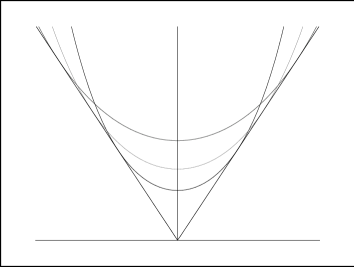
Figure 2: Catenaries and envelope

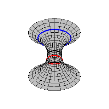
Figure 3: Maximal stability domains

Let ${\mathcal{C}}$ denote the catenoid ${\mathcal{C}}_{1}$ and let $F(t,\omega)$ denote the immersion $F(1,t,\omega)$.

Proposition 4.4

The $n$-dimensional catenoid ${\mathcal{C}}$ in $\mathbb{R}^{n+1}$ has the following properties.

1. The half catenoid ${\mathcal{C}}_{+}:=F([0,T_{n}[,S^{n-1})$ is weakly stable.

2. Let $z$ be the unique positive zero of the Jacobi field $e$. The domain ${\mathcal{D}}_{z}:=F(]-z,z[,S^{n-1})$ is a maximal weakly stable domain (any larger domain has index at least $1$). It is bounded by the two spheres where the catenoid ${\mathcal{C}}$ touches the envelope of the family.

3. The catenoid ${\mathcal{C}}$ has index $1$.

Proof. Assertions 1 and 2 follow immediately from the properties of the vertical and variation Jacobi fields and from Properties 2.3 and 2.4. See Figures 3 and 5.

Assertion 3 has been proved in [3] using the fact that the horizontal half-catenoids are stable, see Figure 5, and in [13] by another method. $\Box$

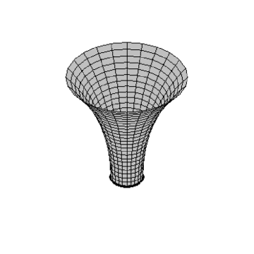
Figure 4: Stable vertical half

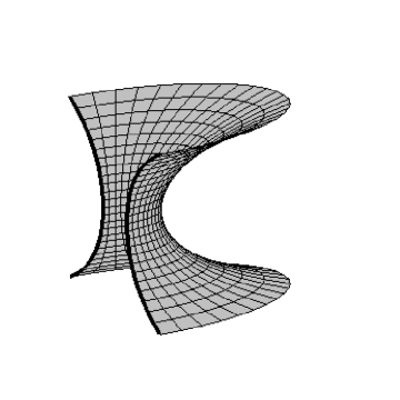
Figure 5: Stable horizontal half

Theorem 4.5

For $n\geq 3$, the $n$-dimensional catenoid ${\mathcal{C}}$ in $\mathbb{R}^{n+1}$ does not satisfy Lindelöf’s property. More precisely, letting $z$ be the positive zero of the Jacobi field $e$, there exists an $\ell\in]0,z[$ such that the following properties hold.

1. The domain ${\mathcal{D}}^{\prime}_{\ell}:=F(]-\ell,\infty[,S^{n-1})$ is weakly stable.

2. For any $\alpha>\ell$, there exists $\beta(\alpha)\in]0,\infty[$ such that the domain ${\mathcal{D}}_{\alpha,\beta(\alpha)}:=F(]-\alpha,\beta(\alpha)[,S^{n-1})$ is a maximal weakly stable domain. In particular, for $\alpha>\ell$, the domain ${\mathcal{D}}^{\prime}_{\alpha}:=F(]-\alpha,\infty[,S^{n-1})$ has index $1$.

3. When it exists, the maximal weakly stable domain ${\mathcal{D}}_{\alpha,\beta(\alpha)}$ is given by Lindelöf’s construction. More precisely, the tangents to the catenary $t\mapsto\big{(}c(t),t\big{)}$ at the two points $\big{(}c(\alpha),-\alpha\big{)}$ and $\big{(}c(\beta(\alpha)),\beta(\alpha)\big{)}$ meet on the axis of the catenary.

Proof.

We introduce the Jacobi field

$$w(\alpha,t):=v(\alpha)e(t)+e(\alpha)v(t).$$

Because $e$ is even and $v$ odd, it follows that $w(\alpha,-\alpha)=0$. Since $w(\alpha,0)=-v(\alpha)<0$ and $\lim_{t\to T_{n},\,t<T_{n}}w(\alpha,t)=e(\alpha)+T_{n}v(\alpha)$ (use (4.25) and (4.26)). Since $n\geq 3$, the value $T_{n}$ is finite and we introduce the Jacobi field $y(t)=e(t)+T_{n}v(t)$. We have $y(0)=-1$ and $y(z)=T_{n}v(z)$. It follows that $y$ has one (and only one) zero $\ell\in]0,z[$. For $\alpha\leq\ell$, we have that $y(\alpha)\leq 0$ and we may conclude that $w(\alpha,\cdot)$ does not vanish on $]-\alpha,\infty[$. On the other-hand, when $\alpha>\ell$, $w(\alpha,\cdot)$ has a unique positive zero $\beta(\alpha)$.

3) Writing the equations for the tangents to the catenary at the points $\big{(}c(\alpha),-\alpha\big{)}$ and $\big{(}c(\beta),\beta\big{)}$, we see that a necessary and sufficient condition for the tangents to intersect on the axis of the catenary is

$$\alpha+\beta=\frac{c(\alpha)}{c_{t}(\alpha)}+\frac{c(\beta)}{c_{t}(\beta)}.$$

Writing that $w(\alpha,\beta)=0$ we find the same necessary and sufficient condition. This proves the last assertion. $\Box$

The following figures illustrate the difference between the case $n\geq 3$ (Figures 7 and 7) and the case $n=2$.

When $n\geq 3$, the construction of the maximal weakly stable domains with tangents and the fact that the height of the catenoids is bounded shows that Lindelöf’s property does not hold.

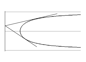
Figure 6: ${\mathcal{D}}_{\alpha,\beta(\alpha)},\leavevmode\nobreak\ n\geq 3$

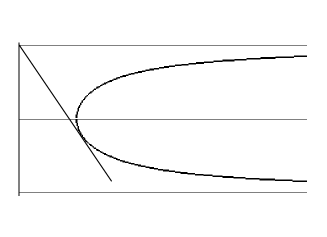
Figure 7: ${\mathcal{D}}^{\prime}_{\ell},\leavevmode\nobreak\ n\geq 3$

5 Catenoids in $\mathbb{H}^{2}\times\mathbb{R}$

Catenoids in $\mathbb{H}^{2}\times\mathbb{R}$ have been studied in [10, 3]. We take the ball model for $\mathbb{H}^{2}$ and we let $\rho$ denote the hyperbolic distance to $0$. We equip $\widehat{M}=\mathbb{H}^{2}\times\mathbb{R}$ with the product metric $\widehat{g}$.

5.1 Preliminaries

In this Section, we review the computations of [3].

The catenoids in $\mathbb{H}^{2}\times\mathbb{R}$ are generated by catenaries $C_{1}(a,\rho)=\big{(}\tanh(\rho),\lambda(a,\rho)\big{)}$ in a vertical plane $\gamma\times\mathbb{R}$, where $\gamma$ is a complete geodesic in $\mathbb{H}^{2}$, and where

(5.27) $$\lambda(a,\rho)=\sinh(a)\,\int_{a}^{\rho}\big{(}\sinh^{2}(t)-\sinh^{2}(a)\big{)}^{-1/2}\,dt,\leavevmode\nobreak\ a>0.$$

As a matter of fact, $C_{1}(a,\rho)$ describes a half-catenary and the whole catenary can be parametrized in the arc-length parameter $s$, by

(5.28) $$C_{2}(a,s)=\big{(}\tanh(R(a,s)/2),\Lambda(a,s)\big{)}$$

where the function $R(a,s)$ and $\Lambda(a,s)$ are smooth and, respectively even and odd. They satisfy the relations

(5.29) $$\left\{\begin{array}[]{ll}R(a,s)&=a+\cosh(a)\int_{0}^{s}\sinh(t)\big{(}\cosh^{2}(a)\cosh^{2}(t)-1\big{)}^{-1/2}\,dt,\\[7.0pt] \cosh(R(a,s))&=\cosh(a)\cosh(s)\text{ \leavevmode\nobreak\ and\leavevmode\nobreak\ }R(a,s)\geq a,\\[7.0pt] \Lambda(a,s)&=\sinh(a)\displaystyle\int_{0}^{s}(\cosh^{2}(a)\cosh^{2}(t)-1)^{-1/2}\,dt,\\[7.0pt] \Lambda_{s}^{2}+R_{s}^{2}&\equiv 1.\\ \end{array}\right.$$

The family $\{{\mathcal{C}}_{a}\}_{a>0}$ of catenoids in $\mathbb{H}^{2}\times\mathbb{R}$ is given (in the ball model) by

(5.30) $$X(a,s,\theta)=\begin{pmatrix}\tanh(R(a,s)/2)\omega_{\theta}\\[6.0pt] \Lambda(a,s)\\ \end{pmatrix}.$$

The metric $X^{*}\widehat{g}$ induced by $X$ on ${\mathcal{C}}_{a}$ is $ds^{2}+\sinh^{2}(R(a,s))d\theta^{2}$ and the unit normal is given by

(5.31) $$N(a,s,\theta)=\begin{pmatrix}\dfrac{\Lambda_{s}}{2\cosh^{2}(R(a,s)/2)}\omega_{\theta}\\ \\ R_{s}\\ \end{pmatrix},$$

where $\Lambda_{s}=\frac{\partial\Lambda}{\partial s}$ and $R_{s}=\frac{\partial R}{\partial s}$.

5.2 Jacobi fields

$\bullet$ The vertical Jacobi field is the function

(5.32) $$v(a,s)=\widehat{g}(\frac{\partial}{\partial t},N)=R_{s}.$$

Taking (5.29) into account, we find

(5.33) $$v(a,s)=\cosh(a)\sinh(s)\big{(}\cosh^{2}(a)\cosh^{2}(s)-1\big{)}^{-1/2}.$$

Note that $v(a,0)=0$ and $v(a,\infty)=1$.

$\bullet$ We take the variation Jacobi field to be

(5.34) $$e(a,s)=-\widehat{g}(\frac{\partial X}{\partial a}(a,s,\theta),N(a,s,\theta)).$$

This Jacobi field has been computed in [3]. We have

$$e(a,s)=\Lambda_{s}R_{a}-\Lambda_{a}R_{s},\text{\leavevmode\nobreak\ \leavevmode\nobreak\ and}$$

(5.35) $$\begin{array}[]{ll}e(a,s)=&\sinh^{2}(a)\cosh(s)\big{(}\cosh^{2}(a)\cosh^{2}(s)-1\big{)}^{-1}\cdots\\ &\hphantom{xxxxx}-v(a,s)\displaystyle\int_{0}^{s}B(a,t)\,dt,\end{array}$$

where

$$B(a,t):=\cosh(a)\sinh^{2}(t)\big{(}\cosh^{2}(a)\cosh^{2}(t)-1\big{)}^{-3/2}.$$

5.3 Stable domains on ${\mathcal{C}}_{a}$

Define the rotation invariant domains

(5.36) $${\mathcal{D}}_{\pm}=X(a,\mathbb{R}_{\pm},[0,2\pi]),\leavevmode\nobreak\ \text{and}$$

(5.37) $${\mathcal{D}}_{\alpha}=X(a,]-\alpha,\alpha[,[0,2\pi]).$$

In [3], we proved the following result.

Theorem 5.1

The catenaries ${\mathcal{C}}_{a}\subset\mathbb{H}^{2}\times\mathbb{R}$ have the following properties.

1. The domains ${\mathcal{D}}_{\pm}$ are weakly stable.

2. The function $e(a,s)$ has a unique positive zero $z(a)$, and

   • ${\mathcal{D}}_{\alpha}$ is stable for $0<\alpha<z(a)$.

   • $J_{{\mathcal{C}}_{a}}$ has eigenvalue $0$ in ${\mathcal{D}}_{z(a)}$ with Dirichlet boundary conditions.

   • ${\mathcal{D}}_{\alpha}$ is unstable for $\alpha>z(a)$.

3. For all $a>0$, the catenoid ${\mathcal{C}}_{a}$ has index $1$.

Sketch of the proof of Theorem 5.1.

Assertion 1 follows from Property 2.4, using the Jacobi field $v(a,s)$ which does not vanish in the interior of ${\mathcal{D}}_{\pm}$.

Assertion 2 is a consequence of Property 2.1 and the fact that the function $e(a,s)$ has a (unique) zero on $]0,+\infty[$. Note that the uniqueness of the positive zero of $e(a,s)$ is a consequence of Assertion 1.

Assertion 3. We refer to [3]. $\Box$

Theorem 5.2

The catenoids ${\mathcal{C}}_{a}$ in $\mathbb{H}^{2}\times\mathbb{R}$ do not satisfy Lindelöf’s property: the domains ${\mathcal{D}}_{\pm}$ are not maximally weakly stable. More precisely, there exists a unique $\ell(a)\in]0,z(a)[$ such that ${\mathcal{D}}^{\prime}_{\ell(a)}:=X(a,]-\ell(a),\infty[,[0,2\pi])$ is maximally weakly stable among rotationally invariant domains.

Proof. For $\alpha>0$, introduce the Jacobi field

(5.38) $$e(a,\alpha,s)=v(a,\alpha)e(a,s)+e(a,\alpha)v(a,s)$$

where $e$ and $v$ are given by (5.32) and (5.35).

Because the vertical Jacobi field $v$ does not vanish on $]0,\infty[$ and on $]-\infty,0[$, we have that $e(a,\alpha,\cdot)$ has at most one zero on these intervals (see also Theorem 5.1, Assertion 1). Oberve that $e(a,\alpha,-\alpha)=0$ and that $e(a,\alpha,0)=v(a,\alpha)>0$. It follows that $e(a,\alpha,\cdot)$ has a zero in $]0,\infty[$ if and only if $e(a,\alpha,\cdot)$ is negative near infinity. Using (5.38), we can write $e(a,s)=f(a,s)-v(a,s)\int_{0}^{s}B(a,t)\,dt$ where $f(a,s)=\sinh^{2}(a)\cosh(s)\big{(}\cosh^{2}(a)\cosh^{2}(s)-1\big{)}^{-1}$, $f(a,0)=1$, $f(a,\infty)=0$ and $B(a,t)=\cosh(a)\sinh^{2}(t)\big{(}\cosh^{2}(a)\cosh^{2}(t)-1\big{)}^{-3/2}$. Let $E(a)=\int_{0}^{\infty}B(a,t)\,dt$, a positive finite value. Using these notations, we have

$$e(a,\alpha,s)=v(a,\alpha)f(a,s)+v(a,s)[e(a,\alpha)-v(a,\alpha)\int_{0}^{s}B(a,t)\,dt].$$

The sign of $e(a,\alpha,s)$ near $+\infty$ is given by the sign of $e(a,\alpha)-E(a)v(a,\alpha)$.

$\rhd$  If $\alpha>z(a)$ (the unique positive zero of the variation Jacobi field $e(a,\cdot)$, then $e(a,\alpha)<0$ so that $e(a,\alpha)-E(a)v(a,\alpha)<0$ and hence $e(a,\alpha,s)$ must have a zero $\beta(\alpha)\in]0,\infty[$. Clearly, we must have $0<\beta(\alpha)<z(a)$. This is not surprising in view of Theorem 5.1, Assertion 2.

$\rhd$  If $\alpha=z(a)$, then $e(a,z(a),s)=v(a,z(a))e(a,s)$ has two zeroes $\pm z(a)$.

$\rhd$  If $0<\alpha<z(a)$, consider the Jacobi field $w(t):=e(a,t)-E(a)v(a,t)$. We have $w(0)=1$ and $w(z(a))=-E(a)v(a,z(a))<0$ so that $w$ has a unique positive zero $\ell(a)\in]0,z(a)[$. When $0<\alpha<\ell(a),w(\alpha)>0$ and hence $X(a,]-\alpha,\infty[,[0,2\pi]$ is weakly stable. For $\alpha>\ell(a),w(a)<0$, $e(a,\alpha,\cdot)$ has a positive zero $\beta(\alpha)$ and $X(a,]-\alpha,\beta(\alpha)[,[0,2\pi]$ is a maximal weakly stable domain. $\Box$

Remark. One could show that ${\mathcal{D}}_{\ell(a)}$ is maximally weakly stable by using a conformal transformation. This method does not apply in higher dimension whereas the above one does.

6 Catenoids in $\mathbb{H}^{n}\times\mathbb{R}$

We consider the space $\mathbb{H}^{n}\times\mathbb{R}$ with the product metric $\widehat{g}=g_{h}+dt^{2}$ and we work with the ball model for $(\mathbb{H}^{n},g_{h})$.

We consider a rotation hypersurface about the axis $\mathbb{R}$, with parametrization

(6.39) $$F(t,\omega)=\big{(}\tanh(f(t)/2)\omega,t\big{)}$$

where $f(t)>0$ is the hyperbolic distance to the axis. Using the flux formula (see Appendix A), we obtain easily the following differential equation for minimal rotation hypersurfaces in $\mathbb{H}^{n}\times\mathbb{R}$,

(6.40) $$\sinh^{n-1}\big{(}f(t)\big{)}\big{(}1+f_{t}^{2}(t)\big{)}^{-1/2}=C$$

for some constant $C$, where $f_{t}$ denotes the derivative of $f$ with respect to $t$.

Differentiating this equation, we have that $f$ also satisfies the equation

(6.41) $$\sinh\big{(}f(t)\big{)}f_{tt}(t)-(n-1)\cosh\big{(}f(t)\big{)}\big{(}1+f_{t}^{2}\big{)}=0.$$

Lemma 6.1

The Cauchy problem

(6.42) $$\left\{\begin{array}[]{lll}\sinh\big{(}f(t)\big{)}f_{tt}(t)&=&(n-1)\cosh\big{(}f(t)\big{)}\big{(}1+f_{t}^{2}\big{)},\\ f(0)&=&a,\\ f_{t}(0)&=&0,\\ \end{array}\right.$$

has a maximal solution of the form $\big{(}]-T(a),T(a)[,f(a,t)\big{)}$ where $t\mapsto f(a,t)$ is a smooth, even function of $t$. Furthermore, the function $f$ satisfies

(6.43) $$\left\{\begin{array}[]{lll}\sinh^{n-1}\big{(}f(a,t)\big{)}\big{(}1+f_{t}^{2}\big{)}^{-1/2}&=&\sinh^{n-1}(a),\\ f(a,t)&\geq&a,\text{ \leavevmode\nobreak\ for all\leavevmode\nobreak\ }t,\\ f_{t}\text{ \leavevmode\nobreak\ \leavevmode\nobreak\ has the sign of\leavevmode\nobreak\ }t.\\ \end{array}\right.$$

For $t\geq 0$, we have

$$f_{t}(a,t)=\big{(}\dfrac{\sinh^{2n-2}(f(a,t))-\sinh^{2n-2}(a)}{\sinh^{2n-2}(a)}\big{)}^{1/2}$$

and the function $f(a,\cdot)$ is a bijection from $[0,T(a)[$ to $[a,\infty[$. Let $\lambda(a,\cdot):[a,\infty[\to[0,T(a)[$ be the inverse function to $f$. Then

(6.44) $$\lambda(a,\rho)=\sinh^{n-1}(a)\int_{a}^{\rho}\big{(}\sinh^{2n-2}(u)-\sinh^{2n-2}(a)\big{)}^{-1/2}\,du$$

which shows that the value $T(a)$ is finite,

(6.45) $$T(a)=\sinh^{n-1}(a)\int_{a}^{\infty}\big{(}\sinh^{2n-2}(u)-\sinh^{2n-2}(a)\big{)}^{-1/2}\,du$$

It follows from the preceding formulas that

(6.46) $$f_{t}\big{(}1+f_{t}^{2}\big{)}^{-1/2}=\mathrm{sgn}(t)\big{(}1-(\frac{\sinh(a)}{\sinh(f)})^{2n-2}\big{)}^{1/2}.$$

Jacobi fields

The normal to the catenoid is given by

(6.47) $$N(a,t,\omega)=(1+f_{t}^{2})^{-1/2}\big{(}-\frac{\omega}{2\cosh^{2}(f/2)},f_{t}\big{)}.$$

It follows that the vertical Jacobi field $v(a,t)$ is an odd function of $t$ which satisfies

(6.48) $$\left\{\begin{array}[]{ll}v(a,t)&:=\widehat{g}(N,\frac{\partial}{\partial t})=f_{t}\big{(}1+f_{t}^{2}\big{)}^{-1/2}\\[6.0pt] &=\mathrm{sgn}(t)\big{(}1-(\frac{\sinh(a)}{\sinh(f)})^{2n-2}\big{)}^{1/2},\\[6.0pt] v(a,0)&=0,\leavevmode\nobreak\ \leavevmode\nobreak\ \lim_{t\to T(a)}v(a,t)=1.\\ \end{array}\right.$$

The variation Jacobi field $e(a,t)$ is an even function of $t$ which satisfies

(6.49) $$\left\{\begin{array}[]{ll}e(a,t)&:=\widehat{g}(N,\frac{\partial F}{\partial a})=-f_{a}\big{(}1+f_{t}^{2}\big{)}^{-1/2}\\[6.0pt] &=f_{t}(1+f_{t}^{2})^{-1/2}\lambda_{a}(a,f),\text{ \leavevmode\nobreak\ for\leavevmode\nobreak\ }t\geq 0,\\[6.0pt] v(a,0)&=-1.\\ \end{array}\right.$$

Note that the second equality follows from the fact that $f(a,\lambda(a,\rho))\equiv\rho$ for $\rho>a$.

It follows from Equation (6.44) that

$$\begin{array}[]{ll}\lambda_{a}(a,\rho)&=-\;\frac{\sinh(\rho)}{\sinh(a)}\frac{\cosh(a)}{\cosh(\rho)}\big{(}(\frac{\sinh(\rho)}{\sinh(a)})^{2n-2}-1\big{)}^{-1/2}+\leavevmode\nobreak\ \leavevmode\nobreak\ \cdots\\[8.0pt] &\hphantom{xxxx}+\cosh(a)\int_{1}^{\sinh(\rho)/\sinh(a)}(v^{2n-2}-1)^{-1/2}(\sinh^{2}(a)v^{2}+1)^{-3/2}\,dv.\end{array}$$

Using the above expressions, we find that for $t\geq 0$,

$$\begin{array}[]{ll}e(a,t)&=-\;\frac{\cosh(a)}{\cosh(f)}\big{(}\frac{\sinh(a)}{\sinh(f)}\big{)}^{n-2}+\leavevmode\nobreak\ \leavevmode\nobreak\ \cdots\\[6.0pt] &\hphantom{xxx}v(a,t)\cosh(a)\int_{1}^{\sinh(f)/\sinh(a)}(v^{2n-2}-1)^{-1/2}(\sinh^{2}(a)v^{2}+1)^{-3/2}\,dv.\end{array}$$

We write the preceding equality as

(6.50) $$\left\{\begin{array}[]{ll}e(a,t)&=:-e_{0}(a,t)+v(a,t)e_{1}(a,t),\text{ \leavevmode\nobreak\ where,}\\[6.0pt] e_{0}(a,t)&:=\frac{\cosh(a)}{\cosh(f)}\big{(}\frac{\sinh(a)}{\sinh(f)}\big{)}^{n-2},\text{ \leavevmode\nobreak\ positive and even,}\\[6.0pt] e_{0}(a,0)&=1,\leavevmode\nobreak\ \leavevmode\nobreak\ e_{0}(a,T(a)-)=0,\\[6.0pt] e_{1}(a,0)&=\cosh(a)\int_{1}^{\sinh(f)/\sinh(a)}(v^{2n-2}-1)^{-1/2}(\sinh^{2}(a)v^{2}+1)^{-3/2}\,dv\\[6.0pt] e_{1}(a,0)&=0,\leavevmode\nobreak\ \leavevmode\nobreak\ e_{1}(a,T(a)-)=E(a),\\[6.0pt] \end{array}\right.$$

where $E(a):=\cosh(a)\int_{1}^{\infty}(v^{2n-2}-1)^{-1/2}(\sinh^{2}(a)v^{2}+1)^{-3/2}\,dv$ is a finite, positive value.

Proposition 6.2

The vertical Jacobi field $v(a,t)$ only vanishes at $t=0$. As a consequence, the half-vertical catenoids ${\mathcal{C}}_{a,\pm}:=F(a,\mathbb{R}_{\pm},S^{n-1})$ are weakly stable.
The variation Jacobi field $e(a,t)$ has exactly one positive zero $z(a)\in]0,T(a)[$. As a consequence the domain ${\mathcal{D}}_{z(a)}:=F(a,]-z(a),z(a)[,S^{n-1})$ is a maximal weakly stable domain.

Proof. The proof is clear in view of Properties 2.3 and 2.4. Note that the fact that $e(a,\cdot)$ has a unique positive zero follows from the positivity of $v(a,\cdot)$ in $]0,\infty[$ and Sturm intertwining zeroes theorem. $\Box$

We now introduce the Jacobi field

$$e(a,\alpha,t):=v(a,\alpha)e(a,t)+e(a,\alpha)v(a,t).$$

Notice that $e(a,\alpha,-\alpha)=0$ and that $e(a,\alpha,0)=-v(a,\alpha)<0$, so that $e(a,\alpha,\cdot)$ cannot have another zero on $]-\infty,0[$. For $t\geq 0$, consider the Jacobi field

$$y(a,t):=e(a,t)+E(a)v(a,t).$$

We have that

$$y(a,\alpha)=\lim_{t\to T(a)-}e(a,\alpha,t).$$

It is clear that $y(a,\cdot)$ has a unique zero on $]0,\infty[$, namely some $\ell(a)\in]0,z(a)[$ (where $z(a)$ is the positive zero of $e(a,\cdot)$).

For $0<\alpha\leq\ell(a)$, we have that $y(a,\alpha)\leq 0$ and hence that $e(a,\alpha,t)<0$ for $t$ close enough to $T(a)$. This implies that for such values of $\alpha$, the function $v(a,\alpha,\cdot)$ cannot vanish on $]0,T(a)[$. For $\alpha>\ell(a)$, we have that $y(a,\alpha)>0$ so that $e(a,\alpha,\cdot)$ has a (unique) zero $\beta(\alpha)\in]0,T(a)[$.

We have proved,

Proposition 6.3

With the above notations,

1. the domain ${\mathcal{D}}^{\prime}_{\ell(a)}:=F(a,]-l(a),T(a)[,S^{n-1})$ is a maximal rotationally symmetric weakly stable domain,

2. the domain ${\mathcal{D}}_{\alpha,\beta(\alpha)}:=F(a,]-\alpha,\beta(\alpha)[,S^{n-1})$ is a maximal weakly stable domain.

7 Catenoids and catenoid cousins in $\mathbb{H}^{3}$

7.1 Hyperbolic computations

We work in the half-space model for the hyperbolic space,

(7.51) $$\mathbb{H}^{3}_{\{x_{1},x_{2},x_{3}\}}=\{(x_{1},x_{2},x_{3})\in\mathbb{R}^{3}\leavevmode\nobreak\ |\leavevmode\nobreak\ x_{3}>0\},\hskip 14.22636ptg_{h}=x_{3}^{-2}\big{(}dx_{1}^{2}+dx_{2}^{2}+dx_{3}^{2}\big{)}.$$

In the hyperbolic plane

(7.52) $$\mathbb{H}^{2}_{\{x,z\}}=\{(x,z)\in\mathbb{R}^{2}\leavevmode\nobreak\ |\leavevmode\nobreak\ z>0\},\hskip 14.22636ptg_{h}=z^{-2}\big{(}dx^{2}+dz^{2}\big{)},$$

we consider the Fermi coordinates $(u,v)$ defined as follows (see Figure 8). Given a point $m=m(x,z)$, let $m^{\prime}$ be its orthogonal projection on the vertical geodesic $\gamma=\{(0,e^{t})\leavevmode\nobreak\ |\leavevmode\nobreak\ t\in\mathbb{R}\}\subset\mathbb{H}^{2}_{\{x,z\}}$. Let $u$ denote the signed hyperbolic distance $d_{h}(m,m^{\prime})$ and $v$ the signed hyperbolic distance $d_{h}(m^{\prime},i)$ (where $i=(0,1)$).

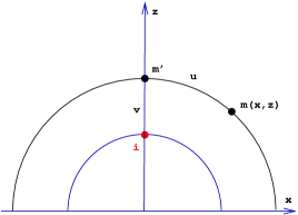
Figure 8: Hyperbolic $2$-plane

The following formulas relate the coordinates $(x,z)$ to the coordinates $(u,v)$.

(7.53) $$\begin{array}[]{lll}\left\{\begin{array}[]{lll}x&=&e^{v}\tanh(u),\\ z&=&\dfrac{e^{v}}{\cosh(u)},\\ \end{array}\right.&\text{ \leavevmode\nobreak\ and\leavevmode\nobreak\ }&\left\{\begin{array}[]{lll}u&=&\arg\sinh(\dfrac{x}{z}),\\ v&=&\dfrac{1}{2}\ln(x^{2}+z^{2}).\\ \end{array}\right.\\ \end{array}\vskip 12.0pt plus 4.0pt minus 4.0pt$$

In the coordinates $\{u,v\}$, the hyperbolic metric is given by

(7.54) $$g_{h}=du^{2}+\cosh^{2}(u)dv^{2}.$$

7.2 Rotation surfaces in $\mathbb{H}^{3}$

We consider a curve $f(t)=(t,f(t))$ in the plane $\mathbb{H}^{2}_{\{u,v\}}$ and the corresponding rotation surface $F:M\looparrowright\mathbb{H}^{3}_{\{x_{1},x_{2},x_{3}\}}$,

(7.55) $$F(t,\theta)=\begin{pmatrix}e^{f(t)}\tanh(t)\cos\theta\\[6.0pt] e^{f(t)}\tanh(t)\sin\theta\\[6.0pt] \dfrac{e^{f(t)}}{\cosh(t)}\\ \end{pmatrix}.$$

We will use the notation

(7.56) $$F(t,\theta)=\begin{pmatrix}e^{f(t)}\tanh(t)\,\omega_{\theta}\\[6.0pt] \dfrac{e^{f(t)}}{\cosh(t)}\\ \end{pmatrix}$$

where $\omega_{\theta}=(\cos\theta,\sin\theta)$ for short, and we denote $(-\sin\theta,\cos\theta)$ by $\dot{\omega}_{\theta}$.

The metric induced on $M$ from the immersion $F$ is given by the matrix

(7.57) $$G_{F}(t,\theta)=\begin{pmatrix}1+\cosh^{2}(t)f_{t}^{2}(t)&0\\[6.0pt] 0&\sinh^{2}(t)\\ \end{pmatrix},$$

where $f_{t}$ denotes the derivative of the function $f$ with respect to the variable $t$.

The unit normal vector $N_{F}$ to the immersion is given by

(7.58) $$N_{F}(t,\theta)=\frac{e^{f(t)}}{\big{(}1+\cosh^{2}(t)f_{t}^{2}(t)\big{)}^{1/2}}\begin{pmatrix}-(\frac{f_{t}(t)}{\cosh(t)}-\frac{\sinh(t)}{\cosh^{2}(t)})\,\omega_{\theta}\\[6.0pt] f_{t}(t)\tanh(t)+\frac{1}{\cosh^{2}(t)}\\ \end{pmatrix}.$$

The principal curvatures of the surface $M$ with respect to $N_{F}$ are given by

(7.59) $$\left\{\begin{array}[]{lll}k_{p}(t)&=&\dfrac{f_{tt}(t)\cosh(t)+2f_{t}(t)\sinh(t)+f_{t}^{3}(t)\cosh^{2}(t)\sinh(t)}{\big{(}1+\cosh^{2}(t)f_{t}^{2}(t)\big{)}^{3/2}}\,,\\ &&\\ k_{n}(t)&=&\dfrac{f_{t}(t)\cosh^{2}(t)}{\sinh(t)\big{(}1+\cosh^{2}(t)f_{t}^{2}(t)\big{)}^{1/2}}\,,\\ \end{array}\right.$$

where $k_{p}$ is the curvature of the generating curve in the hyperbolic plane $\mathbb{H}^{2}$ (see for example [11]).

$\blacktriangleright$ [Notes]

See Notes [090223].

[Notes] $\blacktriangleleft$

Taking these computations into account, the mean curvature of the rotation surface $M$ is given by

(7.60) $$H(t)\sinh(2t)=\frac{d}{dt}\;\frac{f_{t}(t)\sinh(t)\cosh^{2}(t)}{\big{(}1+\cosh^{2}(t)f_{t}^{2}(t)\big{)}^{1/2}}.$$

When $H$ is assumed to be constant, Equation (7.60) provides a first integral for the generating curves of rotation surfaces with constant mean curvature $H$ in the plane $\mathbb{H}^{2}_{\{u,v\}}$. These generating curves come in a family $C_{H,a}$ and will be called $H$-catenaries. The corresponding surfaces ${\mathcal{C}}_{H,a}$ will be called $H$-catenoids. They depend on a real parameter $a$.

More precisely, we will consider three cases, depending on the value of the mean curvature, $H=0$, $H=1$ and $0<H<1$. As a matter of fact, we could consider the cases $0\leq H<1$ and $H=1$, but the case $H=0$ is of particular importance.

We begin by general considerations.

7.2.1 General computations

Consider a graph $G$, $\varphi(a,t)=(t,\lambda(a,t))$ in the plane $\mathbb{H}^{2}_{\{u,v\}}$, see Figure 9. Assume that the curve extends by symmetry with respect to the $u$-axis as a smooth curve and that the extended curve admits an arc-length parametrization of the form

(7.61) $$\Phi(a,s)=\big{(}y(a,s),\Lambda(a,s)\big{)}$$

where $y(a,s)$ is a smooth even function of $s$ and $\Lambda(a,s)$ a smooth odd function of $s$, such that $\Lambda(a,s):=\lambda\big{(}a,y(a,s)\big{)}$ for $s\geq 0$.

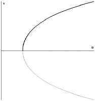
Figure 9: Curve in $\mathbb{H}^{2}$

The corresponding rotation surfaces in $\mathbb{H}^{3}$ are given by the parametrizations

(7.62) $$\begin{array}[]{lll}Y(a,s,\theta)&=&\begin{pmatrix}e^{\Lambda(a,s)}\tanh(y(a,s))\,\omega_{\theta}\\[6.0pt] \dfrac{e^{\Lambda(a,s)}}{\cosh(y(a,s))}\\ \end{pmatrix}.\\ \end{array}$$

The parameter $s$ is the arc-length parameter along the generating curve if and only if the following identity holds,

(7.63) $$1\equiv y_{s}^{2}+\cosh^{2}(y)\Lambda_{s}^{2}=y_{s}^{2}\big{(}1+\cosh^{2}(y)\lambda_{t}^{2}(a,y)\big{)},$$

where $y$ and $\Lambda$ stand respectively for $y(a,s)$ and $\Lambda(a,s)$ and where subscripts indicate differentiation.

According to (7.58), the unit normal vectors along the immersions are given by the formula

(7.64) $$N_{Y}(a,s,\theta)=e^{\Lambda(a,s)}\begin{pmatrix}-(\frac{\Lambda_{s}}{\cosh(y)}-y_{s}\frac{\sinh(y)}{\cosh^{2}(y)})\,\omega_{\theta}\\[6.0pt] \Lambda_{s}\tanh(y)+\frac{y_{s}}{\cosh^{2}(y)}\\ \end{pmatrix},$$

where $y$ stands for $y(a,s)$.

$\blacktriangleright$ [PB3]

[PB3] $\blacktriangleleft$

Having in mind the fact that we will work with minimal or constant mean curvature immersions, we now define Jacobi fields on the surface $M$ in the parametrization $Y$.

7.2.2 Jacobi fields

Recall that the function $y(a,s)$ is assumed to be even and that the function $\Lambda(a,s)$ is assumed to be odd.

$\bullet$ The Killing field associated with the hyperbolic translations along the vertical geodesic $t\mapsto(0,0,e^{t})$ in $\mathbb{H}^{3}_{\{x_{1},x_{2},x_{3}\}}$ is just the position vector. The vertical Jacobi field is the function

(7.65) $$v_{Y}(a,s)=g_{h}(Y,N_{Y})$$

given by the hyperbolic scalar product of the position vector $Y$ with the unit normal vector to the immersion at $Y$.

Property 7.1

The vertical Jacobi field $v_{Y}(a,s)=g_{h}(Y,N_{Y})$ is an odd function of $s$ given by

(7.66) $$v_{Y}(a,s)=\cosh(y(a,s))y_{s}(a,s).$$

$\bullet$ The variation Jacobi field is defined as the hyperbolic scalar product of the variation vector-field of the family with the unit normal vector, $e_{Y}(a,s)=g_{h}(Y_{a},N_{Y})$. We have

(7.67) $$Y_{a}(a,s,\theta)=e^{\Lambda(a,s)}\begin{pmatrix}(\Lambda_{a}\tanh(y)+\frac{y_{a}}{\cosh^{2}(y)})\,\omega_{\theta}\\[6.0pt] \frac{\Lambda_{a}}{\cosh(y)}-y_{a}\frac{\sinh(y)}{\cosh^{2}(y)}\\ \end{pmatrix}.$$

Property 7.2

The variation Jacobi field $e_{Y}(a,s)$ is an even function of $s$ given by

(7.68) $$e_{Y}(a,s)=g_{h}(Y_{a},N_{Y})=\cosh(y(a,s))\big{(}\Lambda_{a}y_{s}-\Lambda_{s}y_{a}\big{)}.$$

$\blacktriangleright$ [PB3]

[PB3] $\blacktriangleleft$

$\blacktriangleright$ [PB2]

[PB2] $\blacktriangleleft$

We now look into the three cases, $H=0$, $H=1$ and $0<H<1$.

7.3 Minimal catenoids in $\mathbb{H}^{3}$

7.3.1 Basic formulas

When $H=0$, Equation (7.60) yields the solutions curves $C_{0,a}$ (the lower index $0$ refers to the value of $H$), for $a\geq 0$,

(7.69) $$\lambda_{0}(a,t)=\sinh(2a)\int_{a}^{t}\dfrac{d\tau}{\cosh(\tau)\big{(}\sinh^{2}(2\tau)-\sinh^{2}(2a)\big{)}^{1/2}}$$

which are defined for $t\geq a$. Notice that this parametrization only covers a half-catenary and that we work up to a $v$-translation in $\mathbb{H}^{2}_{\{u,v\}}$, i.e. up to a hyperbolic translation with respect to the vertical geodesic in $\mathbb{H}^{2}_{\{x,z\}}$.

The arc-length parameter along the curve is given by

(7.70) $$S_{0}(a,t)=\int_{a}^{t}\frac{\sinh(2\tau)\,d\tau}{\big{(}\cosh^{2}(2\tau)-\cosh^{2}(2a)\big{)}^{1/2}}$$

or

(7.71) $$\cosh(2a)\cosh\big{(}2S_{0}(a,t)\big{)}=\cosh(2t),t\geq a.$$

Proposition 7.3

For $s\in\mathbb{R}$, define the functions $y_{0}(a,s)$ and $\Lambda_{0}(a,s)$ by the formulas

(7.72) $$\left\{\begin{array}[]{lll}y_{0}(a,s)&=&a+\displaystyle\int_{0}^{s}\frac{\cosh(2a)\sinh(2t)}{\big{(}\cosh^{2}(2a)\cosh^{2}(2t)-1\big{)}^{1/2}}\,dt\\ \text{and}&&\\ \Lambda_{0}(a,s)&=&\sqrt{2}\sinh(2a)\displaystyle\int_{0}^{s}\frac{\big{(}\cosh(2a)\cosh(2t)-1\big{)}^{1/2}}{\big{(}\cosh^{2}(2a)\cosh^{2}(2t)-1\big{)}}\,dt.\\ \end{array}\right.$$

1. The function $y_{0}$ is an even function of $s$ and $\Lambda_{0}$ an odd function of $s$.

2. For $s\geq 0$, the function $y_{0}(a,\cdot)$ is the inverse function of the function $S_{0}(a,\cdot)$. In particular,

   $$\cosh\big{(}2y_{0}(a,s)\big{)}=\cosh(2a)\,\cosh(2s).$$

3. For $s\geq 0$, we have $\Lambda_{0}(a,s)=\lambda_{0}(a,y_{0}(a,s))$.

4. For $s\in\mathbb{R}$, the functions $s\mapsto\big{(}y_{0}(a,s),\Lambda_{0}(a,s)\big{)}$ are arc-length parametrizations of the family of catenaries $C_{0,a},a>0$.

Proof. The proof is straightforward. $\Box$

For later reference, we introduce the function

(7.73) $$J_{0}(a,t)=\sinh(2a)(\cosh(2a)\cosh(2t)+1)^{-1}(\cosh(2a)\cosh(2t)-1)^{-1/2},$$

so that $\Lambda_{0}(a,s)=\sqrt{2}\int_{0}^{s}J_{0}(a,t)\,dt$. We compute $\frac{\partial J_{0}}{\partial a}(a,t)$ and we find,

(7.74) $$\left\{\begin{array}[]{ll}I_{0}(a,t)&=\dfrac{\partial J_{0}}{\partial a}(a,t)=\dfrac{n(\cosh(2a),\cosh(2t))}{d(\cosh(2a),\cosh(2t))},\text{\leavevmode\nobreak\ where}\\ &\\ n(A,T)&=A(3-A^{2})T^{2}+(A^{2}-1)T-2A,\\[6.0pt] d(A,T)&=(AT+1)^{2}(AT-1)^{3/2}.\\ \end{array}\right.$$

We note that $n(A,T)$ is a polynomial of degree $2$ in $T$.

$\blacktriangleright$ [Notes]

(see Notes [090318]).

[Notes] $\blacktriangleleft$

Lemma 7.4

Let $a_{1}>0$ be such that $\cosh^{2}(2a_{1})=\frac{11+8\sqrt{2}}{7}\approx 3.1876$, i.e. $a_{1}\approx 0.5915$. For $a\geq a_{1}$ and for all $t$, we have $n(cosh(2a),\cosh(2t))\leq 0$.

To the above family $C_{0,a},a>0$ of catenaries corresponds a family ${\mathcal{C}}_{0,a},a>0$ of catenoids in $\mathbb{H}^{3}$ with the arc-length parametrization $Y_{0}(a,s,\theta)$,

(7.75) $$Y_{0}(a,s,\theta)=\begin{pmatrix}e^{\Lambda_{0}}\tanh(y_{0})\,\omega_{\theta}\\[6.0pt] e^{\Lambda_{0}}/\cosh(y_{0})\\ \end{pmatrix}$$

where the functions $\Lambda_{0}(a,s)$ and $y_{0}(a,s)$ are given by Proposition 7.3.

Catenoids in $\mathbb{H}^{3}$ have been considered in [9, 4] and more recently in [12]. A new phenomenon has been pointed out by these authors, namely that among the family ${\mathcal{C}}_{0,a}$ of catenoids in $\mathbb{H}^{3}$, there are stable and index one catenoids. We now give a precise analysis of this phenomenon and we also consider Lindelöf’s property for catenoids in $\mathbb{H}^{3}$.

7.3.2 Jacobi fields on ${\mathcal{C}}_{0,a}$

According to (7.64), the unit normal $N_{0}(a,s,\theta)$ on ${\mathcal{C}}_{0,a}$ is given by

(7.76) $$N_{0}(a,s,\theta)=\dfrac{e^{\Lambda_{0}}}{\cosh(y_{0})}\,\begin{pmatrix}-n_{1}\,\omega_{\theta}\\[6.0pt] n_{2}\\ \end{pmatrix}$$

where

$$\left\{\begin{array}[]{ll}n_{1}(a,s)&=\Lambda_{0,s}-y_{0,s}\tanh(y_{0}),\leavevmode\nobreak\ y_{0,s}=\frac{\partial y_{0}}{\partial s},\\[8.0pt] n_{2}(a,s)&=\Lambda_{0,s}\sinh(y_{0})+y_{0,s}/\cosh(y_{0}).\\ \end{array}\right.$$

Applying the formulas (7.66) and (7.68) of Section 7.2.2, we have the expressions for the vertical and variation Jacobi fields on ${\mathcal{C}}_{0,a}$.

The variation Jacobi field $e_{0}(a,s)$ is given by

(7.77) $$e_{0}(a,s)=-g_{h}(Y_{0,a}(a,s,\theta),N_{0}(a,s,\theta))=-\cosh(y_{0})\big{(}\Lambda_{0,a}y_{0,s}-\Lambda_{0,s}y_{0,a}\big{)}.$$

We obtain

(7.78) $$\begin{array}[]{ll}e_{0}(a,s)=&\dfrac{\sinh^{2}(2a)\cosh(2s)}{\big{(}\cosh^{2}(2a)\cosh^{2}(2s)-1\big{)}}\leavevmode\nobreak\ \leavevmode\nobreak\ \leavevmode\nobreak\ \cdots\\[6.0pt] &\hphantom{xxxxxxx}\cdots\leavevmode\nobreak\ \leavevmode\nobreak\ \leavevmode\nobreak\ -\dfrac{\cosh(2a)\sinh(2s)}{\big{(}\cosh(2a)\cosh(2s)-1\big{)}^{1/2}}\displaystyle\int_{0}^{s}I_{0}(a,t)\,dt\end{array}$$

where $I_{0}(a,t)$ is defined by (7.74).

The vertical Jacobi field $v_{0}(a,s)$ is given by

(7.79) $$v_{0}(a,s)=\sqrt{2}\widehat{g}(Y_{0}(a,s,\theta),N_{0}(a,s,\theta))=\sqrt{2}\cosh(y_{0})y_{0,s}.$$

It follows that

(7.80) $$v_{0}(a,s)=\cosh(2a)\sinh(2s)\big{(}\cosh(2a)\cosh(2s)-1\big{)}^{-1/2}.$$

Let

(7.81) $$f_{0}(a,s)=\sinh^{2}(2a)\cosh(2s)\big{(}\cosh^{2}(2a)\cosh^{2}(2s)-1\big{)}^{-1}$$

an even function of $s$ which goes to $0$ at infinity. In view of Equations (7.78), (7.80) and (7.81), we have

(7.82) $$e_{0}(a,s)=f_{0}(a,s)-v_{0}(a,s)\int_{0}^{s}I_{0}(a,t)\,dt.$$

Observe that the integral

(7.83) $$E_{0}(a):=\int_{0}^{\infty}I_{0}(a,t)\,dt$$

exists for all values of $a$.

7.3.3 Stable domains on ${\mathcal{C}}_{0,a}$

We can now investigate the stability properties of the catenoids ${\mathcal{C}}_{0,a}$ in $\mathbb{H}^{3}$.

Lemma 7.5

The half-catenoids

(7.84) $${\mathcal{D}}_{0,a,\pm}=Y_{0}(a,\mathbb{R}_{\pm},[0,2\pi])$$

are weakly stable. It follows from this property that a Jacobi field $w(a,s)$ which only depends on the radial variable $s$ on ${\mathcal{C}}_{0,a}$ can have at most one zero on $\mathbb{R}^{\bullet}_{+}$ and on $\mathbb{R}^{\bullet}_{-}$.

Proof. Use Property 2.4 and the fact that $v_{0}(a,s)$ is a Jacobi field which only vanishes at $s=0$. $\Box$

Lemma 7.6

The half-catenoids $Y_{0}(a,\mathbb{R},]\varphi,\varphi+\pi[)$ are weakly stable. Negative eigenvalues of the Jacobi operator $J_{{\mathcal{C}}_{0,a}}$ on domains of revolution are necessarily associated with eigenfunctions depending only on the parameter $s$. The catenoids ${\mathcal{C}}_{0,a}$ have at most index $1$.

Proof. The fact that the index of ${\mathcal{C}}_{a}$ is at most $1$ has been proved by [12] using the same method as in [13]. Alternatively, one could use Jacobi fields associated to geodesics orthogonal to the axis of the catenoids. $\Box$

$\blacktriangleright$ [Notes]

See Ricardo’s notes 090509-rsa-lindeloef-killing.tex.

[Notes] $\blacktriangleleft$

We can now state the main theorem of this section. Recall that the number $E_{0}(a)$ is defined by (7.83) and that the Jacobi fields $v_{0}(a,s)$ and $e_{0}(a,s)$ are given respectively by (7.80) and (7.78), with the relation (7.82).

Theorem 7.7

Let ${\mathcal{C}}_{0,a}$ be the family of catenoids in $\mathbb{H}^{3}$ given by (7.75).

1. The index of the catenoid ${\mathcal{C}}_{0,a}$ depends on the value of the integral $E_{0}(a)$ defined by (7.83). More precisely, if $E_{0}(a)\leq 0$ then the catenoid ${\mathcal{C}}_{0,a}$ is stable, if $E_{0}(a)>0$, then the catenoid ${\mathcal{C}}_{0,a}$ has index $1$.

2. When ${\mathcal{C}}_{0,a}$ has index $1$, there exist $0<z(a)$ such that

   $${\mathcal{D}}_{0,z(a)}=Y_{0}(a,]-z(a),z(a)[,[0,2\pi])$$

   is a maximal weakly stable domain.

3. When ${\mathcal{C}}_{0,a}$ has index $1$, there exist $0<\ell(a)<z(a)$ such that

   $${\mathcal{D}}_{0,\ell(a)}=Y_{0}(a,]-\ell(a),\infty[,[0,2\pi])$$

   is a maximal weakly stable rotation invariant domain.

4. The catenoids ${\mathcal{C}}_{0,a}$ do not satisfy Lindelöf’s property.

5. There exist two numbers $0<a_{2}<a_{1}$ such that for all $a>a_{1}$, the catenoids ${\mathcal{C}}_{0,a}$ are stable, and for all $a<a_{2}$, the catenoids ${\mathcal{C}}_{0,a}$ have index $1$.

Proof.

Assertion 1. As stated in Lemma 7.5, the function $e_{0}(a,s)$ can have at most one zero on $]0,\infty[$ and at most one zero on $]-\infty,0[$. Observe that the function $e_{0}(a,s)$ is even and that $e_{0}(a,0)=1$. To determine whether $e_{0}$ has a zero, it suffices to look at its behaviour at infinity. If $E_{0}(a)>0$, the function $e_{0}(a,s)$ tends to $-\infty$ at infinity so that it has exactly two symmetric zeroes in $\mathbb{R}$. This implies that the index of ${\mathcal{C}}_{0,a}$ is at least $1$. Using Lemma 7.6, we conclude that ${\mathcal{C}}_{0,a}$ has index $1$. If $E_{0}(a)<0$, the function $e_{0}(a,s)$ tends to $+\infty$ at infinity so that it is always positive and the catenoid ${\mathcal{C}}_{0,a}$ is stable. Assume now that $E_{0}(a)=0$. We then have the relation

$$e_{0}(a,s)=f_{0}(a,s)+v_{0}(a,s)\int_{s}^{\infty}I_{0}(a,t)\,dt.$$

Using Equation (7.74), we see that $I_{0}(a,t)$ is positive for $t$ large enough provided that $\cosh^{2}(2a)\leq 3$. In that case, it follows that $e_{0}(a,s)$ is positive at infinity and hence that ${\mathcal{C}}_{0,a}$ is stable. If $E(a)=0$ and $\cosh^{2}(2a)>3$, we need to look at the behaviour of $e_{0}(a,s)$ at infinity more precisely. When $s$ tends to $+\infty$, we have

$$f_{0}(a,s)\sim 2\tanh^{2}(2a)e^{-2s},\leavevmode\nobreak\ \leavevmode\nobreak\ v_{0}(a,s)\sim\sqrt{\frac{\cosh(2a)}{2}}e^{s},\text{\leavevmode\nobreak\ \leavevmode\nobreak\ \leavevmode\nobreak\ and}$$

$$\int_{s}^{\infty}I_{0}(a,t)\,dt\sim\frac{2^{3/2}(3-\cosh^{2}(2a))}{3\cosh^{5/2}(2a)}e^{-3s}.$$

It follows that $e_{0}(a,s)\sim\frac{4}{3}e^{-2s}$ is positive at infinity and hence that ${\mathcal{C}}_{0,a}$ is stable. This proves Assertion 1.

Assertion 2. Saying that ${\mathcal{C}}_{0,a}$ has index $1$ is equivalent to saying the $E_{0}(a)>0$ and hence that $e_{0}$ as two symmetric zeroes. This proves Assetion 2.

Assertion 3. Given any $\alpha>0$, we introduce the Jacobi field $e_{0}(a,\alpha,s)$,

(7.85) $$e_{0}(a,\alpha,s)=v_{0}(a,\alpha)e_{0}(a,s)+e_{0}(a,\alpha)v_{0}(a,s).$$

This Jacobi field vanishes at $s=-\alpha<0$ so that it cannot vanish elsewhere in $]-\infty,0[$ and can at most vanish once in $]0,\infty[$. Using Equations (7.85) and (7.82), we can write

(7.86) $$e_{0}(a,\alpha,s)=v_{0}(a,\alpha)f_{0}(a,s)+v_{0}(a,s)\big{[}e_{0}(a,\alpha)-v_{0}(a,\alpha)\int_{0}^{s}I_{0}(a,t)\,dt\big{]}.$$

We have

$$e_{0}(a,\alpha,-\alpha)=0\text{\leavevmode\nobreak\ and\leavevmode\nobreak\ }e_{0}(a,\alpha,0)=v_{0}(a,\alpha)>0$$

so that $e_{0}(a,\alpha,\cdot)$ vanishes in $]0,\infty[$ if and only if $e_{0}(a,\alpha)-v_{0}(a,\alpha)E_{0}(a)<0$ (recall that $E_{0}(a)=\int_{0}^{\infty}I_{0}(a,t)\,dt$).

If ${\mathcal{C}}_{0,a}$ is stable, then clearly $e_{0}(a,\alpha,\cdot)$ cannot vanish twice in $\mathbb{R}$.

Assume that ${\mathcal{C}}_{0,a}$ has index $1$ or, equivalently, that $E_{0}(a)>0$. In that case, $e_{0}(a,\cdot)$ has exactly one positive zero $z(a)$.

$\rhd$ For $\alpha>z(a)$, $e_{0}(a,\alpha)<0$ so that $e_{0}(a,\alpha)-v_{0}(a,\alpha)E_{0}(a)<0$ and $e_{0}(a,\alpha,\cdot)$ has a positive zero $\beta$ (which must satisfy $\beta<z(a)$).

$\rhd$ For $\alpha=z(a)$, $e_{0}(a,\alpha,s)=v_{0}(a,\alpha)e_{0}(a,s)$ has two zeroes $\pm z(a)$.

$\rhd$ For $0<\alpha<z(a)$, we can argue as follows. Consider the Jacobi field $w(a,t)=e_{0}(a,t)-E_{0}(a)v_{0}(a,t)$. At $t=0$, we have $w(a,0)=1$ and at $t=z(a)$, we have $w(a,z(a))<0$ because $e_{0}(a,z(a))=0$, $E_{0}(a)>0$ and $v_{0}(a,z(a))>0$. It follows that $w(a,t)$ has a unique zero in $]0,z(a)[$ and hence that there exists a value $\ell(a)>0$ such that

$${\mathcal{D}}_{0,\ell(a)}=Y_{0}(a,]-\ell(a),\infty[,[0,2\pi])$$

is a maximal weakly stable rotation invariant domain. This proves Assertion 3.

Assertion 4. This follows immediately from the previous assertion.

Assertion 5. The first part of the Assertion follows from Lemma 7.4 which implies that $e(a,s)$ never vanishes when $a>a_{1}$. To prove the second part of Assertion 3, we can either use the fact that $E_{0}(a)$ tends to $+\infty$ when $a$ tends to zero from above or use the criteria given in [4] (Corollary 5.13, p. 708) or [12] (Corollary 4.2), see Section 7.3.4. $\Box$

$\blacktriangleright$ [Notes]

See Ricardo’s notes catenoids-h3-v8.pdf version 8, Theorem 1, page 9.

[Notes] $\blacktriangleleft$

We have the following geometric interpretation of Theorem 7.7

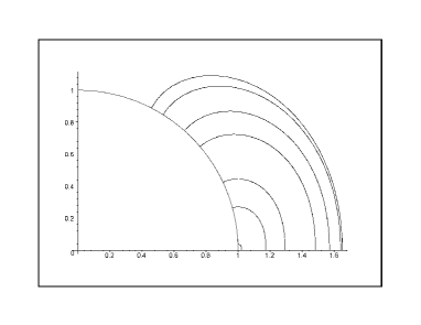
Figure 10: Foliating

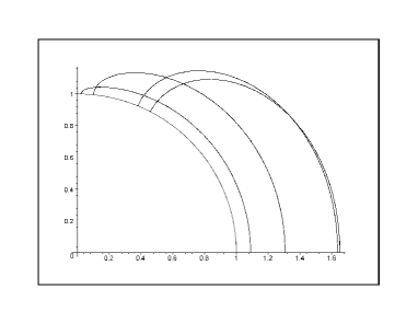
Figure 11: Intersecting

Proposition 7.8

We have the following geometric interpretation.

• Let ${\mathcal{S}}$ be an open interval on which $E_{0}<0$ (hence the catenoid ${\mathcal{C}}_{0,a}$ is stable for all $a\in{\mathcal{S}}$). For $a\in{\mathcal{S}}$, the catenaries $C_{0,a}$ locally foliate the hyperbolic plane $\mathbb{H}^{2}_{\{u,v\}}$.

• Let ${\mathcal{U}}$ be an open interval on which $E_{0}>0$ (hence the catenoid ${\mathcal{C}}_{0,a}$ has index $1$ for all $a\in{\mathcal{U}}$). For $a,b\in{\mathcal{U}}$, the catenaries $C_{0,a}$ and $C_{0,b}$ in $\mathbb{H}^{2}_{\{u,v\}}$ intersect exactly at two points. Furthermore, the family $\{C_{0,a}\}_{a\in{\mathcal{U}}}$ has an envelope. Furthermore, the points at which ${\mathcal{C}}_{0,a}$ touches the envelope correspond to the maximal stable domain ${\mathcal{D}}_{0,z(a)}$.

Proof.

Define the $v$-height function of the catenoid ${\mathcal{C}}_{0,a}$ by

(7.87) $$V_{0}(a)=\lim_{t\to\infty}\lambda_{0}(a,t)=\lim_{s\to\infty}\Lambda_{0}(a,s).$$

Lemma 7.9

Let $a_{2}>a_{1}>0$ be two values of the parameter $a$. The catenaries $C_{0,a_{1}}$ and $C_{0,a_{2}}$ intersect at most at two symmetric points and they do so if and only if $V_{0}(a_{2})>V_{0}(a_{1})$.

Proof. To prove the Lemma, consider the difference $w(t):=\lambda_{0}(a_{2},t)-\lambda_{0}(a_{1},t)$ for $t\geq a_{2}>a_{1}$. A straightforward computation shows that this function increases from the negative value $-\lambda_{0}(a_{1},a_{2})$ (achieved for $t=a_{2}$) to $V_{0}(a_{2})-V_{0}(a_{1})$ (the limit at $t=\infty$). It follows that $w$ has at most one zero and does so if and only if $V_{0}(a_{2})-V_{0}(a_{1})>0$.

The Proposition follows from the fact that $V_{0}(a)=\sqrt{2}\int_{0}^{\infty}J_{0}(a,t)\,dt$ and that $V^{\prime}_{0}(a)=\sqrt{2}E_{0}(a)$ where $E_{0}(a)$ is defined by (7.83). $\Box$

Figure 12: Intersecting

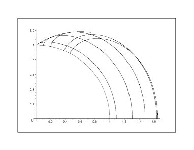
Figure 13: With envelope

Observation.  One can also define the $x$-height function of the catenoid ${\mathcal{C}}_{0,a}$ by

(7.88) $$X_{0}(a)=\lim_{s\mapsto\infty}e^{\Lambda_{0}(a,s)}\tanh(y_{0}(a,s))=e^{\sqrt{2}\int_{0}^{\infty}J_{0}(a,t)\,dt},$$

where $J_{0}(a,t)$ is defined by (7.73).

The critical points of $X_{0}(a)$ correspond to the zeroes of the function $E_{0}(a)$.

$\blacktriangleright$ [Notes]

See [090318] for more details.

[Notes] $\blacktriangleleft$

7.3.4 Numerical computations

Remarks.

1.  The graph (maple plot) of the function $a\mapsto E(a)$, for $a>0$ (see Figure 15) shows that there exists some $a_{0}\approx 0,4955\cdots$ such that

• for $a\geq a_{0}$, the catenoids ${\mathcal{C}}_{0,a}$ are stable and the corresponding catenaries locally foliate the hyperbolic plane,

• for $a<a_{0}$, the catenoids ${\mathcal{C}}_{0,a}$ have index $1$,

• the function $E_{0}(a)$ has a unique zero $a_{0}$ which is the unique critical point of $x$-height function $X_{0}(a)$. The properties of the family of catenoids change at the point $a_{0}$, from an intersecting family to a foliating family.

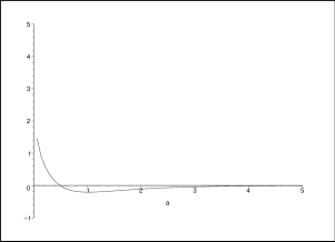
Figure 14: Graph $E_{0}(a)$

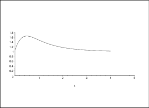
Figure 15: Graph $X_{0}(a)$

2.  The family of minimal catenoids in $\mathbb{H}^{3}$ has been described for the first time by H. Mori. To perform the computations, he used the representation of $\mathbb{H}^{3}$ as a hypersurface in the $4$-dimensional Lorentz space. The family of catenoids is described by a function $\phi(\alpha,s)$ ([9], Theorem 1, p. 791) which is the same as our function $\Lambda_{0}(a,s)$, Proposition 7.3, Equation (7.72), if we set $2\alpha=\cosh(2a)$. According to Mori’s Theorem 2 ([9], p. 792), for $\alpha\geq\frac{17}{2}$, i.e. for $a\geq a_{M}:=\mathrm{argcosh}(3)\approx 1.7627\cdots$, the catenoid ${\mathcal{C}}_{0,a}$ is (globally) stable. Mori’s proof relies on the following facts.

• The Jacobi operator on ${\mathcal{C}}_{0,a}$ is given by $J=-\Delta+2-|A|^{2}$, where the norm of the second fundamental form $|A|$ can be expressed in terms of $a,s$.

• The Laplacian is bounded from below, $-\Delta\geq\frac{1}{4}$ on ${\mathcal{C}}_{0,a}$ (this follows from Cheeger’s inequality).

• For $a\geq a_{M}$, we have $|A|^{2}\leq 2+\frac{1}{4}$.

This method for proving stability is far from optimal. This explains why Mori’s bound $a_{M}\approx 1.7627\cdots$ is worse than our bounds $a_{1}\approx 0.5915$ and $a_{0}\approx 0,4955\cdots$.

M. do Carmo and M. Dajczer proved that some catenoids in the family ${\mathcal{C}}_{0,a}$ are not stable. For that purpose, they proved ([4], Corollary 5.13, p. 708) that a stable complete minimal immersion, $M^{n}\looparrowright\mathbb{H}_{n+1}$ with finite total curvature must satisfy the inequality

$$\int_{M}|A_{M}|^{2}\big{(}|A_{M}|^{2}-n(n+1)\big{)}\,d\mu_{M}\leq 0.$$

Taking the explicit form of $|A|$ and $d\mu_{M}$ on the catenoids ${\mathcal{C}}_{0,a}$, the left-hand side of the above inequality give a function of $a$. Plotting this function, one sees that the catenoids ${\mathcal{C}}_{0,a}$ have at least index $1$ for $a\leq a_{CD}\approx 0,4668\cdots$. Using a different criterion, K. Seo slightly improved this bound. The bound $a_{CD}\approx 0,4668\cdots$ is slightly less that our bound $a_{0}\approx 0,4955\cdots$.

$\maltese$  Maple mori-et-alii.mws to be checked !  $\maltese$

7.4 Catenoid cousins in $\mathbb{H}^{3}$

7.4.1 Basic formulas

We now consider catenoid cousins, i.e. constant mean curvature $1$ rotation hypersurfaces in $\mathbb{H}^{3}(-1)$. In this case, the mean curvature equation (7.60) reads

(7.89) $$\sinh(2t)=\frac{d}{dt}\;\frac{f_{t}(t)\sinh(t)\cosh^{2}(t)}{\big{(}1+\cosh^{2}(t)f_{t}^{2}(t)\big{)}^{1/2}}.$$

which yields

$$\frac{f_{t}(t)\sinh(t)\cosh^{2}(t)}{\big{(}1+\cosh^{2}(t)f_{t}^{2}(t)\big{)}^{1/2}}=\frac{1}{2}\cosh(2t)-d,$$

for some constant $d\in\mathbb{R}$. It follows that

$$f_{t}^{2}\cosh^{2}(t)\big{[}\sinh^{2}(2t)-(\cosh(2t)-2d)^{2}\big{]}=\big{[}\cosh(2t)-2d\big{]}^{2}$$

$$f_{t}^{2}\cosh^{2}(t)\big{[}4d\cosh(2t)-1-4d^{2}\big{]}=\big{[}\cosh(2t)-2d\big{]}^{2}.$$

For a solution to exist, $d$ needs to be positive so that we may assume that $2d=e^{-2a}$ for some $a\in\mathbb{R}$, and we get

$$2f_{t}^{2}\cosh^{2}(t)e^{-2a}\big{(}\cosh(2t)-\cosh(2a)\big{)}=\big{(}\cosh(2t)-e^{-2a}\big{)}^{2}.$$

It follows from (7.89) that

(7.90) $$f_{t}=\dfrac{e^{a}\big{(}\cosh(2t)-e^{-2a}\big{)}}{\sqrt{2}\cosh(t)\sqrt{\cosh(2t)-\cosh(2a)}},\leavevmode\nobreak\ \leavevmode\nobreak\ t\geq|a|.$$

$\blacktriangleright$  We now limit ourselves to the embedded case and assume that $a>0$.

Equation (7.90) yields embedded catenary cousins $\{C_{1,a},a>0\}$, given by

(7.91) $$\lambda_{1}(a,t)=\int_{a}^{t}\dfrac{e^{a}\big{(}\cosh(2\tau)-e^{-2a}\big{)}}{\sqrt{2}\cosh(\tau)\sqrt{\cosh(2\tau)-\cosh(2a)}}\,d\tau,\text{ \leavevmode\nobreak\ for\leavevmode\nobreak\ }t\geq a,$$

where the lower index $1$ refers to $H=1$.

Notice that the function $\lambda_{1}$ describes the upper halves of catenary-like curves and that we work up to $v$-translations in $\mathbb{H}^{2}_{\{u,v\}}$, i.e. up to hyperbolic translations along the vertical geodesic $\gamma$ in $\mathbb{H}^{2}_{\{x,z\}}$.

The arc-length function along the curve $C_{1,a}$ is given by

$$S_{1}(a,t)=\int_{a}^{t}\big{(}1+\cosh^{2}(\tau)\lambda_{1,\tau}^{2}(a,\tau)\big{)}^{1/2}\,d\tau$$

i.e.

$$S_{1}(a,t)=\int_{a}^{t}\frac{e^{a}\sinh(2\tau)}{\sqrt{2}\sqrt{\cosh(2\tau)-\cosh(2a)}}\,d\tau.$$

Finally, we arrive at

$$S_{1}(a,t)=\frac{e^{a}}{\sqrt{2}}\sqrt{\cosh(2t)-\cosh(2a)}$$

i.e.

(7.92) $$\cosh(2t)=2e^{-2a}S_{1}^{2}(a,t)+\cosh(2a),\leavevmode\nobreak\ \leavevmode\nobreak\ t\geq a.$$

For $s>0$, we can define a positive function $y_{1}(a,s)$ by the relation

$$\cosh\big{(}2y_{1}(a,s)\big{)}=2e^{-2a}s^{2}+\cosh(2a)$$

and we can compute the derivative of the function $s\mapsto\lambda_{1}\big{(}a,y_{1}(a,s)\big{)}$. We obtain the formula

$$\partial_{s}\lambda_{1}\big{(}a,y_{1}(a,s)\big{)}=\frac{\sqrt{2}\big{(}2e^{-2a}s^{2}+\sinh(2a)\big{)}}{(2e^{-2a}s^{2}+\cosh(2a)+1)\sqrt{2e^{-2a}s^{2}+\cosh(2a)-1}}$$

which we can write as

$$\partial_{s}\lambda_{1}\big{(}a,y_{1}(a,s)\big{)}=\frac{e^{a}\big{(}2s^{2}+e^{2a}\sinh(2a)\big{)}}{2(s^{2}+e^{2a}\cosh^{2}(a))\sqrt{s^{2}+e^{2a}\sinh^{2}(a)}}.$$

We can use this formulas to define the functions $y_{1}(a,s)$ and $\Lambda_{1}(a,s)$ over $\mathbb{R}$ as follows.

Proposition 7.10

For $a>0$ and $s\in\mathbb{R}$, define the functions $y_{1}(a,s)$ and $\Lambda_{1}(a,s)$ by the formulas

(7.93) $$y_{1}(a,s)=a+\int_{0}^{s}\frac{2e^{-2a}t\,dt}{\sqrt{\big{(}2e^{-2a}t^{2}+\cosh(2a)\big{)}^{2}-1}},$$

and

(7.94) $$\Lambda_{1}(a,s)=\int_{0}^{s}\frac{e^{a}\big{(}2t^{2}+e^{2a}\sinh(2a)\big{)}\,dt}{2\big{(}t^{2}+e^{2a}\cosh^{2}(a)\big{)}\sqrt{t^{2}+e^{2a}\sinh^{2}(a)}}.$$

1. The function $y_{1}$ is smooth, even, and satisfies

   $$\cosh(2y_{1}(a,s))=2e^{-2a}s^{2}+\cosh(2a).$$

2. The function $\Lambda_{1}$ is smooth, odd, and satisfies $\Lambda_{1}(a,s)=\lambda_{1}(a,y_{1}(a,s))$ for $s\geq 0$.

3. For $a>0$, the maps $\mathbb{R}\ni s\mapsto\big{(}y_{1}(a,s),\Lambda_{1}(a,s)\big{)}\in\mathbb{H}^{2}_{\{u,v\}}$ are arc-length parametrizations of the family of embedded catenary cousins $\{C_{1,a}\}_{a>0}$ which generate the family $\{{\mathcal{C}}_{1,a}\}_{a>0}$ of embedded catenoid cousins (rotation surfaces with constant mean curvature $1$ in $\mathbb{H}^{3}(-1)$).

4. The parametrization of the family $\{{\mathcal{C}}_{1,a}\}_{a>0}$ in $\mathbb{H}^{3}_{\{x_{1},x_{2},x_{3}\}}$, is given by

   (7.95) $$Y_{1}(a,s)=\begin{pmatrix}e^{\Lambda_{1}(a,s)}\tanh(y_{1}(a,s))\,\omega_{\theta}\\[6.0pt] e^{\Lambda_{1}(a,s)}\frac{1}{\cosh(y_{1}(a,s))}\\ \end{pmatrix}.\vskip 12.0pt plus 4.0pt minus 4.0pt$$

7.4.2 Jacobi fields on ${\mathcal{C}}_{1,a}$

As in Section 7.2.2, we define the vertical and variation Jacobi fields on ${\mathcal{C}}_{1,a}$.

The vertical Jacobi field $v_{1}(a,s)$ on ${\mathcal{C}}_{1,a}$ is the scalar product of the Killing field of hyperbolic translations along the vertical geodesic $\gamma$ with the unit normal vector to the surface. According to formula (7.66), we have

Lemma 7.11

The vertical Jacobi field $v_{1}$ is a smooth odd function of $s$. It is given by

(7.96) $$v_{1}(a,s)=\cosh(y_{1}(a,s))y_{1,s}(a,s)=\dfrac{e^{-a}s}{\sqrt{s^{2}+e^{2a}\sinh^{2}(a)}}$$

and satisfies $v_{1}(a,0)=0$, $v_{1}(a,\infty)=e^{-a}$.

The variation Jacobi field $e_{1}(a,s)$ on ${\mathcal{C}}_{1,a}$ is the scalar product of the variation field of the family ${\mathcal{C}}_{1,a}$ with the unit normal vector to the surface. According to (7.68), we have

(7.97) $$e_{1}(a,s)=\cosh\big{(}y_{1}(a,s)\big{)}\big{(}\Lambda_{1,a}y_{1,s}-\Lambda_{1,s}y_{1,a}\big{)}(a,s).$$

which we can write as

$$v_{1}(a,s)\Lambda_{1,a}(a,s)-\cosh(y_{1}(a,s))y_{1,a}(a,s)\Lambda_{1,s}(a,s).$$

Using Proposition 7.10 and Lemma 7.11, we find the formula

(7.98) $$\cosh(y_{1})\,\Lambda_{1,s}\,y_{1,a}=\dfrac{\sinh^{2}(2a)-4e^{-4a}s^{4}}{4\big{(}e^{-2a}s^{2}+\cosh^{2}(a)\big{)}\big{(}e^{-2a}s^{2}+\sinh^{2}(a)\big{)}}.$$

By (7.94), we can write $\Lambda_{1}(a,s)$ as $\int_{0}^{s}A(a,t)\,dt$, where the integrand $A(a,t)$ is

(7.99) $$\left\{\begin{array}[]{lll}A(a,t)&=&\dfrac{2e^{a}t^{2}+e^{3a}\sinh(2a)}{2\big{(}t^{2}+e^{2a}\cosh^{2}(a)\big{)}\big{(}t^{2}+e^{2a}\sinh^{2}(a)\big{)}^{1/2}},\\[8.0pt] &=&\dfrac{A_{1}(a,t)}{2A_{2}(a,t)A_{3}^{1/2}(a,t)},\\ \end{array}\right.$$

where the second equality defines the functions $A_{i}$.

One can now compute the derivative of $A(a,t)$ with respect to the variable $a$.

$$A_{a}(a,t)=\dfrac{A_{1,a}(a,t)}{2A_{2}(a,t)A_{3}^{1/2}(a,t)}-\dfrac{A_{1}(a,t)B_{2}(a)}{2A_{2}^{2}(a,t)A_{3}^{1/2}(a,t)}-\dfrac{A_{1}(a,t)B_{3}(a)}{4A_{2}(a,t)A_{3}^{3/2}(a,t)},$$

where

$$B_{2}(a)=\partial_{a}\big{(}e^{2a}\cosh^{2}(a)\big{)},\leavevmode\nobreak\ \leavevmode\nobreak\ B_{3}(a)=\partial_{a}\big{(}e^{2a}\sinh^{2}(a)\big{)}.$$

It follows that

$$\begin{array}[]{ll}A_{a}(a,t)=&\dfrac{2e^{a}t^{2}+e^{3a}(3\sinh(2a)+2\cosh(2a))}{2A_{2}(a,t)A_{3}^{1/2}(a,t)}-\dfrac{A_{1}(a,t)B_{2}(a)}{2A_{2}^{2}(a,t)A_{3}^{1/2}(a,t)}\leavevmode\nobreak\ \leavevmode\nobreak\ \cdots\\[6.0pt] &\hphantom{xxxxxx}-\dfrac{A_{1}(a,t)B_{3}(a)}{4A_{2}(a,t)A_{3}^{3/2}(a,t)},\\ \end{array}$$

i.e.

(7.100) $$\left\{\begin{array}[]{l}A_{a}(a,t)=B(a,t)-C(a,t),\text{ \leavevmode\nobreak\ where\leavevmode\nobreak\ }\\ B(a,t),C(a,t)>0,\text{ \leavevmode\nobreak\ for\leavevmode\nobreak\ }a>0,t\in\mathbb{R},\\ B(a,t)\sim\frac{e^{a}}{|t|},\text{ \leavevmode\nobreak\ at infinity,}\\ C(a,t)=O(\frac{1}{|t|^{3}}),\text{ \leavevmode\nobreak\ at infinity.}\\ \end{array}\right.$$

Finally, with the above notations, we can write the variation Jacobi field as

$$\begin{array}[]{ll}e_{1}(a,s)=&\;-\,\dfrac{e^{4a}\sinh^{2}(a)\cosh^{2}(a)-s^{4}}{\big{(}s^{2}+e^{2a}\cosh^{2}(a)\big{)}\big{(}s^{2}+e^{2a}\sinh^{2}(a)\big{)}}\,-\,v_{1}(a,s){\displaystyle\int_{0}^{s}C(a,t)\,dt}+\leavevmode\nobreak\ \leavevmode\nobreak\ \cdots\\ &\\ &\hphantom{xxxxx}\cdots\leavevmode\nobreak\ \leavevmode\nobreak\ +v_{1}(a,t){\displaystyle\int_{0}^{s}B(a,t)\,dt}\\ \end{array}$$

We have proved,

Lemma 7.12

The variation Jacobi field $e_{1}$ is a smooth, even function of $s$ which can be written as

(7.101) $$e_{1}(a,s)=-f_{1}(a,s)+v_{1}(a,s){\displaystyle\int_{0}^{s}B(a,t)\,dt},$$

where the function $f_{1}$ is a smooth, even function of $s$, such that $f_{1}(a,0)=1$ and $f_{1}(a,\infty)$ finite. Furthermore,

$$\lim_{s\to\infty}v_{1}(a,s){\displaystyle\int_{0}^{s}B(a,t)\,dt}=+\infty.$$

$\blacktriangleright$ [PB2]

$\maltese$  Computations to be checked !  $\maltese$

[PB2] $\blacktriangleleft$

7.4.3 Stable domains on the embedded catenoid cousins

We can now investigate the stability properties of the embedded catenoids cousins $\{{\mathcal{C}}_{1,a}\}_{a>0}$ in $\mathbb{H}^{3}(-1)$.

Lemma 7.13

The upper and lower halves of the embedded catenoid cousins

(7.102) $${\mathcal{D}}_{1,a,\pm}=Y_{1}(a,\mathbb{R}_{\pm},[0,2\pi]),$$

are weakly stable. It follows from this property that a Jacobi field $w(a,s)$ which only depends on the radial variable $s$ on ${\mathcal{C}}_{1,a}$, for $a>0$, can have at most one zero on $\mathbb{R}^{\bullet}_{+}$ and on $\mathbb{R}^{\bullet}_{-}$.

Proof. Use Property 2.4 and the fact that $v_{1}(a,s)$ is a Jacobi field which only vanishes at $s=0$. $\Box$

Lemma 7.14

The vertical halves of the catenoid cousins $Y_{1}(a,\mathbb{R},]\varphi,\varphi+\pi[)$ are weakly stable. Negative eigenvalues of the Jacobi operator $J_{{\mathcal{C}}_{1,a}}$ on domains of revolution are necessarily associated with eigenfunctions depending only on the parameter $s$. The embedded catenoid cousins ${\mathcal{C}}_{1,a}$ have at most index $1$.

Proof. Consider Jacobi fields associated to geodesics orthogonal to the axis of the catenoids. $\Box$

$\blacktriangleright$ [Notes]

See Ricardo’s notes 090509-rsa-lindeloef-killing.tex.

[Notes] $\blacktriangleleft$

We can now state the main theorem of this section. Recall that the Jacobi fields $v_{1}(a,s)$ and $e_{1}(a,s)$ are given respectively by Lemmas 7.11 and 7.12.

Theorem 7.15

Let $\{{\mathcal{C}}_{1,a},a>0\}$ be the family of embedded catenoid cousins in $\mathbb{H}^{3}$ given by the parametrization $Y_{1}$, Equation (7.95).

1. The Jacobi field $e_{1}(a,s)$ has exactly one positive zero $z_{1}(a)$ and the domains

   $${\mathcal{D}}_{1,a,z_{1}(a)}=Y_{1}(a,]-z_{1}(a),z_{1}(a)[,[0,2\pi])$$

   are maximal weakly stable domains.

2. For any $\alpha>0$, there exists a $\beta(\alpha)>0$ such that the domains

   $${\mathcal{D}}_{1,a,-\alpha,\beta(\alpha)}=Y_{1}(a,]-\alpha,\beta(\alpha)[,[0,2\pi])$$

   are maximal weakly stable domains.

3. In particular, the embedded catenoid cousins $\{{\mathcal{C}}_{1,a}\}_{a>0}$ satisfy Lindelöf’s property: the upper and lower halves of the embedded catenoid cousins ${\mathcal{D}}_{1,a,\pm}$ are maximal rotationally symmetric domains.

4. The index of the catenoid ${\mathcal{C}}_{1,a}$ is equal to $1$.

Proof.

Assertion 1. As we have seen in Lemma 7.13, the function $e_{1}(a,s)$ can have at most one zero on $]0,\infty[$ and at most one zero on $]-\infty,0[$. By Lemma 7.12, the function $e_{1}(a,s)$ is even, $e_{1}(a,0)=-1$ and $e_{1}(a,\infty)=\infty$. It follows that $e_{1}(a,s)$ has exactly two symmetric zeroes in $\mathbb{R}$. This proves Assertion 1.

Assertion 2. Given any $\alpha>0$, we introduce the Jacobi field $e_{1}(a,\alpha,s)$,

(7.103) $$e_{1}(a,\alpha,s)=v_{1}(a,\alpha)e_{1}(a,s)+e_{1}(a,\alpha)v_{1}(a,s).$$

This Jacobi field vanishes at $s=-\alpha<0$ so that it cannot vanish elsewhere in $]-\infty,0[$ and can at most vanish once in $]0,\infty[$. Using Lemma 7.12, we can write

$$e_{1}(a,\alpha,s)=-v_{1}(a,\alpha)f_{1}(a,s)+v_{1}(a,s)\big{(}e_{1}(a,\alpha)+v_{1}(a,\alpha)\int_{0}^{s}B(a,t)\,dt\big{)}.$$

It follows that $e_{1}(a,\alpha,-\alpha)=0$, $e_{1}(a,\alpha,0)<0$ and $\lim_{s\to\infty}e_{1}(a,\alpha,s)=+\infty$, and hence that $e_{1}(a,\alpha,\cdot)$ must vanish at least once. This proves Assertion 2.

Assertion 3. This is a consequence of Assertion 2.

Assertion 4. This assertion follows from Assertion 1 and from Lemma 7.14. This has also been proved, using different methods, by Lima and Rossman [7]. $\Box$

7.5 Surfaces with constant mean curvature $0\leq H<1$

One can also study rotation surfaces with constant mean curvature $H$, $0\leq H<1$ in $\mathbb{H}^{3}(-1)$. This is similar to the case of minimal surfaces.

More precisely, $H$-rotation surfaces in $\mathbb{H}^{3}(-1)$, with $0\leq H<1$, come in a one-parameter family ${\mathcal{C}}_{H,a}$. For some values of $a$ the surfaces are stable, for other values of $a$ they have index $1$. Furthermore, they do not satisfy Lindelöf’s property.

The computations are much more complicated but similar to the minimal case. The functions involved depend continuously on the parameter $H$, for $0\leq H<1$.

7.6 Higher dimensional catenoids

The method described in the previous sections could be applied to study the stable domains on higher dimensional catenoids (minimal rotation hypersurfaces or constant mean curvature $1$ rotation hypersurfaces) in $\mathbb{H}^{n+1}$.

8 Appendix A

In this Appendix, we give a flux formula which is valid in a quite general framework.

Let $M^{n}\looparrowright(\widehat{M}^{n+1},\widehat{g})$ be an isometric embedding with mean curvature vector $\overrightarrow{H}$.

Given a relatively compact domain $D\subset M$, let $\nu$ denote the unit normal to $\partial D$, pointing inwards. We denote by $d\mu_{M}$ the Riemannian measure for the induced metric on $M$ and by $d\mu_{\partial D}$ the Riemannian measure for the induced metric on $\partial D$.

Proposition 8.1

Given any Killing vector-field ${\mathcal{K}}$ on $\widehat{M}$, we have the flux formula,

(8.104) $$n\int_{D}\widehat{g}({\mathcal{K}},\overrightarrow{H})\,d\mu_{M}=-\;\int_{\partial D}\widehat{g}({\mathcal{K}},\nu)\,d\mu_{\partial D}.$$

Proof. Recall that according to [5] (p. 237 ff), the vector-field ${\mathcal{K}}$ is a Killing field on $\widehat{M}$ if and only if $\widehat{g}(\widehat{D}_{X}{\mathcal{K}},X)=0$ for all vector-field $X$ on $\widehat{M}$ (here $\widehat{D}$ is the covariant derivative associated with the Riemannian metric $\widehat{g}$).

Given the Killing field ${\mathcal{K}}$, let $\omega$ be the dual $1$-form, $\omega(\cdot)=\widehat{g}({\mathcal{K}},\cdot)$ and let $\omega_{M}=\omega|_{M}$ be the restriction of $\omega$ to $M$.

The following formula holds,

(8.105) $$\delta_{M}\omega_{M}=-n\;g_{M}({\mathcal{K}},\overrightarrow{H})$$

where $\delta_{M}$ is the divergence in the induced metric on $M$.

Indeed, let $\{E_{i}\}_{1\leq i\leq n}$ be a local onf on $M$, then

$$\begin{array}[]{ll}\delta_{M}\omega_{M}&=-\;\sum_{i}(D_{E_{i}}\omega_{M})(E_{i})\\ &=-\;\sum_{i}[E_{i}\cdot(\omega_{M}(E_{i}))-\omega_{M}(D_{E_{i}}E_{i})]\\ &=-\;\sum_{i}[E_{i}\cdot\widehat{g}({\mathcal{K}},E_{i})+\widehat{g}({\mathcal{K}},D_{E_{i}}E_{i})]\\ &=-n\widehat{g}({\mathcal{K}},\overrightarrow{H})-\;\sum_{i}\widehat{g}(\widehat{D}_{E_{i}}{\mathcal{K}},E_{i})\\ \end{array}$$

which proves Formula (8.105). We can now apply the divergence theorem in $D$,

$$\begin{array}[]{ll}n\int_{D}\widehat{g}({\mathcal{K}},\overrightarrow{H})\,d\mu_{M}&=-\;\int_{D}\delta_{M}(\omega_{M})\,d\mu_{M}\\ &=-\int_{\partial D}\omega_{M}(\nu)\,d\mu_{\partial D}.\end{array}$$

The Proposition follows. $\Box$

$\blacktriangleright$ [Notes]

[090712-divergence-killing-fields-flux.pdf]

[Notes] $\blacktriangleleft$

References

- [1] Lucas Barbosa and Manfredo do Carmo. Stability of minimal surfaces and eigenvalues of the laplacian. Math. Zeit., 173:13–28, 1980.
- [2] Lucas Barbosa, Jonas Gomes, and Alexandre Silveira. Foliation of -dimensional space forms by surfaces with constant mean curvature. Bol. Soc. Bras. Mat., 18:2:1–12, 1987.
- [3] Pierre Bérard and Ricardo Sa Earp. Minimal hypersurfaces in , total curvature and index. arXiv:0808.3838, 2008.
- [4] Manfredo do Carmo and Marcos Dajczer. Hypersurfaces in spaces of constant curvature. Transactions of the American Mathematical Society, 277:685–709, 1983.
- [5] Shoshichi Kobayashi and Katsumi Nomizu. Foundations of differential geometry, Vol. I. Interscience Publishers, 1963.
- [6] H. Blaine Lawson, Jr. Lectures on minimal submanifolds. Vol. I, volume 9 of Mathematics Lecture Series. Publish or Perish Inc., Wilmington, Del., Second edition, 1980.
- [7] Levi Lopes de Lima and Wayne Rossman. On the index of constant mean curvature surfaces in hyperbolic space. Indiana Univ. Math. J., 47:685–723, 1998.
- [8] Lorenz Lindelöf. Sur les limites entre lesquelles le caténoïde est une surface minimale. Mathematische Annalen, 2:160–166, 1870.
- [9] Hiroshi Mori. Minimal surfaces of revolution in and their stability properties. Indiana Univ. Math. J., 30:787–794, 1981.
- [10] Ricardo Sa Earp and Eric Toubiana. Screw motion surfaces in and . Illinois J. Math., 49(4):1323–1362, 2005.
- [11] Ricardo Sa Earp and Eric Toubiana. Introduction à la géométrie hyperbolique et aux surfaces de Riemann. Cassini, Paris, 2009.
- [12] Keomkyo Seo. Stable minimal hypersurfaces in the hyperbolic space. Preprint, 2009.
- [13] Luen-Fai Tam and Detang Zhou. Stability properties of the higher dimensional catenoid in . Proc. Amer. Math. Soc., 137:3451–3461, 2009.
Pierre Bérard
Université Joseph Fourier
Institut Fourier - Mathématiques (UJF-CNRS)
B.P. 74
38402 Saint Martin d’Hères Cedex - France
Pierre.Berard@ujf-grenoble.fr
Ricardo Sa Earp
Departamento de Matemática
Pontifícia Universidade Católica do Rio de Janeiro
22453-900 Rio de Janeiro - RJ - Brazil
earp@mat.puc-rio.br