Modelling CO formation in the turbulent interstellar medium

Abstract

We present results from high-resolution three-dimensional simulations of turbulent interstellar gas that self-consistently follow its coupled thermal, chemical and dynamical evolution, with a particular focus on the formation and destruction of H₂ and CO. We quantify the formation timescales for H₂ and CO in physical conditions corresponding to those found in nearby giant molecular clouds, and show that both species form rapidly, with chemical timescales that are comparable to the dynamical timescale of the gas.

We also investigate the spatial distributions of H₂ and CO, and how they relate to the underlying gas distribution. We show that H₂ is a good tracer of the gas distribution, but that the relationship between CO abundance and gas density is more complex. The CO abundance is not well-correlated with either the gas number density $n$ or the visual extinction $A_{\rm V}$: both have a large influence on the CO abundance, but the inhomogeneous nature of the density field produced by the turbulence means that $n$ and $A_{\rm V}$ are only poorly correlated. There is a large scatter in $A_{\rm V}$, and hence CO abundance, for gas with any particular density, and similarly a large scatter in density and CO abundance for gas with any particular visual extinction. This will have important consequences for the interpretation of the CO emission observed from real molecular clouds.

Finally, we also examine the temperature structure of the simulated gas. We show that the molecular gas is not isothermal. Most of it has a temperature in the range of 10–20 K, but there is also a significant fraction of warmer gas, located in low-extinction regions where photoelectric heating remains effective.

1 Introduction

As essentially all star formation within the Milky Way occurs within cold, dense clouds of molecular gas (Lada & Lada, 2003), understanding how these clouds form, and how and why they then form stars, is crucial if we are to develop any real understanding of the process of star formation (Mac Low & Klessen, 2004; Ballesteros-Paredes et al., 2007; McKee & Ostriker, 2007). Observations of molecular emission lines provide us with a great deal of information on the internal structure and dynamics of molecular clouds, and may also hold important clues to their past dynamical history (Ferriere, 2001).

Traditionally, molecular clouds have been viewed as quasi-static objects that form stars slowly over a long lifetime (Zuckerman & Evans, 1974; Shu, Adams & Lizano, 1987; Krumholz, Matzner & McKee, 2006). In this picture, the dynamical evolution of a cloud and the chemical evolution of the gas within it are only loosely coupled, and can be modelled separately. In the past few years, however, this traditional picture has begun to give way to a new picture of clouds as inherently dynamical entities, whose formation and evolution are dominated by the effects of turbulence (Ballesteros-Paredes et al., 1999; Klessen, Heitsch & Mac Low, 2000; Klessen, 2001; Elmegreen & Scalo, 2004; Scalo & Elmegreen, 2004). The dynamical evolution of the cloud is rapid, with a timescale comparable to those of key chemical processes such as the conversion of atomic to molecular hydrogen (H₂) or the freeze-out of molecules onto the surfaces of interstellar dust grains in dark cores. If this picture is correct, then the dynamics and chemistry of the gas are strongly coupled, with one directly influencing the evolution of the other, and to model them correctly we must model them together.

An additional impetus towards the development of coupled models of molecular cloud dynamics and chemistry comes from the realization that if the internal motions of the clouds are dominated by supersonic turbulence, then it is far more difficult than is often appreciated to infer details of their three-dimensional structure from emission or absorption line observations. Because we see clouds in projection, we have no direct information about the line-of-sight positions of emission or absorption features, only about their radial velocities. In a supersonically turbulent cloud, random velocity variations along the line of sight can create coherent features in position-position-velocity (PPV) space that actually correspond to multiple, physically-separated regions in real space, or, conversely, can break up a real physical feature into multiple distinct features in PPV space (Ballesteros-Paredes & Mac Low 2002; see also Klessen, Heitsch & Mac Low 2000, Heitsch, Mac Low, & Klessen 2001, Federrath et al. 2009). To properly interpret these observations, we need to be able to compare them with simulated observations produced from numerical cloud models that capture the full dynamical and chemical complexity of the clouds and the dense cores within them.

Previous attempts to model cloud formation have not properly addressed the coupling between the cloud dynamics and the cloud chemistry. Most attempts have focussed either on a detailed treatment of cloud chemistry within the framework of a highly simplified dynamical model (e.g. Hennebelle & Pérault, 1999, 2000; Koyama & Inutsuka, 2000, 2002; Bergin et al., 2004) or on a detailed treatment of the dynamics, but without any treatment of the chemistry (e.g. Balsara et al., 2004; Kritsuk & Norman, 2004; Slyz et al., 2005; Hennebelle & Audit, 2007; Hennebelle et al., 2008; Banerjee et al., 2009). Recently, some studies have begun to treat the formation of molecular hydrogen (${\rm H_{2}}$) in high-resolution, three-dimensional simulations of cloud formation (Dobbs, Bonnell, & Pringle, 2006; Dobbs & Bonnell, 2007; Glover & Mac Low, 2007a, b; Dobbs et al., 2008). This is a useful step forward, but although ${\rm H_{2}}$ makes up most of the mass of a giant molecular cloud (GMC), it is very difficult to observe, owing to the weakness of its rotational lines and their large energy separations. Much of what we know about molecular clouds comes instead from observations of carbon monoxide (CO), but until now there has been no attempt to model the far more complex chemistry of CO in a high-resolution three-dimensional simulation.

In this paper, we present a lightweight treatment of gas-phase chemistry and radiative cooling that we have developed to tackle this problem. Our treatment is outlined in Section 2 and includes a simplified model for CO formation and destruction that tracks the abundances of thirty-two distinct chemical species (§2.1), an approximate treatment of ${\rm H_{2}}$ self-shielding and dust extinction that uses the “six-ray” approximation of Glover & Mac Low (2007a, b) (§2.2) and a detailed cooling function (§2.3). We show the results of some tests of the model in Section 3, and discuss the initial conditions used for our simulations in Section 4. In Sections 5–7, we present a few preliminary results of these simulations, concerning the time evolution of the mean chemical abundances (§5), the density and temperature probability distribution functions (§6), and the spatial distribution of molecular hydrogen and CO (§7). We conclude with a brief summary in Section 8.

2 Method

2.1 Basic framework

We solve the equations of fluid flow for a magnetised interstellar gas using a modified version of the ZEUS-MP hydrodynamical code (Norman, 2000; Hayes et al., 2006). An earlier version of this modified code was presented in Glover & Mac Low (2007a). In the present version, we have updated and extended the cooling function, as described in §2.3 below. We have also improved and significantly extended our treatment of gas phase chemistry. We now track the abundances of thirty-two species. Thirteen of these species – ${\rm H^{-}}$, $\rm{H}_{2}^{+}$, $\rm{H}_{3}^{+}$, ${\rm CH}^{+}$, ${\rm CH}_{2}^{+}$, ${\rm OH}^{+}$, $\rm{H_{2}O}^{+}$, ${\rm H_{3}O^{+}}$, ${\rm CO}^{+}$, ${\rm HOC^{+}}$, $\rm{O^{-}}$, ${\rm C^{-}}$ and ${\rm O_{2}^{+}}$ – are assumed to be instantaneously in chemical equilibrium. For the remaining nineteen species – ${\rm e^{-}}$, $\rm{H}^{+}$, ${\rm H}$, ${\rm H_{2}}$, $\rm{He}$, $\rm{He}^{+}$, $\rm{C}$, $\rm{C^{+}}$, $\rm{O}$, $\rm{O}^{+}$, ${\rm OH}$, $\rm{H_{2}O}$, ${\rm CO}$, ${\rm C_{2}}$, $\rm{O}_{2}$, ${\rm HCO^{+}}$, ${\rm CH}$, ${\rm CH}_{2}$ and ${\rm CH}_{3}^{+}$ – we follow the full non-equilibrium evolution.

As in Glover & Mac Low (2007a), we represent the abundance of each of the non-equilibrium species with a tracer field that advects as a density. To ensure consistent advection of the chemical species, such that elemental abundances are conserved locally, as well as globally, we use a modified version of the Consistent Multi-fluid Advection (CMA) algorithm of Plewa & Müller (1999), described in Appendix A. The chemical rate equations governing the creation and destruction of these species are solved in an operator-split fashion, using the implicit integrator DVODE (Brown, Byrne, & Hindmarsh, 1989). The gas energy equation is also operator-split: the effects of any radiative heating or cooling of the gas are combined with those of the pressure-work term into a rate equation that is coupled to the chemical rate equations and so is solved implicitly by DVODE, while the advection of the gas energy density is handled as in the unmodified ZEUS-MP code. For reasons of computational efficiency, we use conservation laws for charge and elemental abundance to determine the abundances of ${\rm e^{-}}$, H, He, C and O, reducing the number of rate equations that DVODE must solve to fifteen (fourteen chemical rate equations plus the energy equation).

To model the chemistry of the gas, we use a chemical network consisting of 218 reactions between 32 species. Details of the reactions included in the network, along with the rate coefficients adopted in each case, are given in Tables 2–8 in Appendix B. Note that in our present study, we include no grain surface reactions other than the formation of ${\rm H_{2}}$ (reaction 165). The chemical effects of grain surface recombination and the freeze-out of CO, ${\rm H_{2}O}$, etc., in dense gas will be treated in future work.

2.2 Photochemistry

To model the photochemistry of optically thin gas, we assume an incident radiation field corresponding to the standard interstellar radiation field, as determined by Draine (1978). This field has a strength $G_{0}=1.7$ in Habing (1968) units, corresponding to an integrated flux of $2.7\times 10^{-3}\>{\rm erg}\>{\rm cm^{-2}}\>{\rm s^{-1}}$. Photodissociation and photoionization rates appropriate for this field strength are listed in Table 7.

In optically thick gas, it is necessary to account for absorption by dust, by the Lyman-Werner lines of ${\rm H_{2}}$ (important for ${\rm H_{2}}$ self-shielding and CO shielding), and by the ultraviolet absorption lines of CO (important for CO self-shielding). To treat these processes with full accuracy in a three-dimensional hydrodynamic simulation is beyond our current capabilities. The problem is one of computational cost: in a hydrodynamical simulation with $N$ fluid elements, the cost of resolving a monochromatic radiation field with the same spatial resolution, and with a comparable angular resolution, is of order $O(N^{5/3})$, as we require $O(N^{2/3})$ rays to fully sample the angular distribution of the radiation field for each of the $N$ fluid elements. To model line absorption, the radiation field must also be discretised in frequency-space, increasing the cost to $O(N_{\nu}\times N^{5/3})$, where $N_{\nu}$ is the number of frequency bins required. In comparison, the cost of modelling the hydrodynamics is only of order $O(N)$. Thus, the cost of properly treating the radiation field in an optically thick $128^{3}$ zone hydrodynamical simulation is $128^{2}N_{\nu}$ times greater than the cost of solving for the hydrodynamical evolution, which is far out of the reach of our current computational resources.

To overcome this problem, we are forced to approximate. The approach that we have chosen to adopt is the “six-ray” method used in Glover & Mac Low (2007a, b), which is based on an original idea by Nelson & Langer (1997). In this approximation, we compute photochemical rates in each zone in our simulation volume by averaging over a small number of lines of sight. Specifically, we compute the column densities of ${\rm H_{2}}$, CO, and H nuclei in all forms (i.e. $N_{\rm H,tot}\simeq N_{\rm H}+2N_{{\rm H_{2}}}+N_{\rm{H}^{+}}$, where $N_{\rm H}$, $N_{{\rm H_{2}}}$ and $N_{\rm{H}^{+}}$ are the column densities of atomic H, molecular ${\rm H_{2}}$, and protons, respectively) in both the positive and negative directions along each of the three coordinate axes of the simulation. For each zone we therefore know the column densities in six different directions (or, alternatively, along six rays).

The rates of most of the reactions listed in Table 7 are sensitive only to the amount of dust extinction, and for a plane-parallel slab geometry, the rates in optically thick gas are related to those in optically thin gas by the expression

$$R_{\rm thick}=R_{\rm thin}f_{\rm dust}\equiv R_{\rm thin}\exp(-\gamma A_{\rm V}),$$ (1)

where $R_{\rm thin}$ is the optically thin rate, $f_{\rm dust}\equiv\exp(-\gamma A_{\rm V})$ is the dust shielding factor, $A_{\rm V}$ is the visual extinction in magnitudes, and where the appropriate value of $\gamma$ for each reaction is listed in Table 7. Using the relationship

$$A_{\rm V}=\frac{N_{\rm H,tot}}{1.87\times 10^{21}\>{\rm cm^{-2}}}$$ (2)

between $A_{\rm V}$ and $N_{\rm H,tot}$, as is appropriate for gas in the diffuse ISM (Draine & Bertoldi, 1996), we can associate a value of $A_{\rm V}$ with each of our six rays for any given zone in our simulation volume. We can then calculate the total rate in that zone, $R_{\rm thick,i}$, as

$$R_{\rm thick,i}=\frac{1}{6}R_{\rm thin}\sum_{j=1}^{6}\exp(-\gamma A_{{\rm V},j}),$$ (3)

where $A_{{\rm V},j}$ is the visual extinction along ray $j$.

To treat the photodissociation of ${\rm H_{2}O^{+}}$ and ${\rm H_{3}O^{+}}$ (reactions 188–195), we use a very similar approach. However, for these reactions the optically thick and optically thin rates are related by the more complicated expression (Sternberg & Dalgarno, 1995),

$$R_{\rm thick}=R_{\rm thin}\exp(-2.55A_{\rm V}+0.0165A_{\rm V}^{2}),$$ (4)

for $A_{\rm V}\leq 15$, and by Equation 1 with $\gamma=2.8$ for $A_{\rm V}>15$. Hence, the total rate in zone $i$ is given in this case by

$$R_{\rm thick,i}=\frac{1}{6}R_{\rm thin}\sum_{j=1}^{6}\left[f_{\rm A}\exp(-2.55A_{{\rm V},j}+0.0165A_{{\rm V},j}^{2})+(1-f_{\rm A})\exp(-2.8A_{{\rm V},j})\right],$$ (5)

where $f_{\rm A}=1$ for $A_{{\rm V},j}\leq 15$, and $f_{\rm A}=0$ for $A_{{\rm V},j}>15$, and where $A_{{\rm V},j}$ is computed in the same manner as before.

To treat ${\rm H_{2}}$ photodissociation accurately, one must take into account not only absorption by dust, but also the effects of ${\rm H_{2}}$ self-shielding. If we assume that the effects of dust absorption and self-shielding can be treated separately, then for a plane-parallel geometry the effects of dust absorption can be modeled by a dust shielding factor given by Equation 1, with $\gamma=3.74$ (Draine & Bertoldi, 1996). Similarly, the effects of ${\rm H_{2}}$ self-shielding can be modeled by a factor (Draine & Bertoldi, 1996)

$$f_{\rm shield}=\frac{0.965}{(1+x/b_{5})^{2}}+\frac{0.035}{(1+x)^{1/2}}\exp\left[-8.5\times 10^{-4}(1+x)^{1/2}\right],$$ (6)

where $x=N_{{\rm H_{2}}}/(5\times 10^{14}\>{\rm cm}^{-2})$, and $b_{5}=b/(10^{5}\>{\rm cm}\>{\rm s}^{-1})$, where $b$ is the Doppler broadening parameter. The fully shielded ${\rm H_{2}}$ photodissociation rate then follows as

$$R_{\rm H_{2},thick}=f_{\rm dust}f_{\rm shield}R_{\rm H_{2},thin}.$$ (7)

Using our six-ray approximation, we can compute $f_{\rm dust}$ and $f_{\rm shield}$ for each ray, and hence can compute the total rate as

$$R_{\rm H_{2},thick,i}=\frac{1}{6}R_{\rm H_{2},thin}\sum_{j=1}^{6}f_{{\rm dust},j}f_{{\rm shield},j}.$$ (8)

Finally, to treat CO photodissociation, it is necessary to take account of three separate contributions to the shielding: CO self-shielding, shielding of CO by the ${\rm H_{2}}$ Lyman-Werner lines, and dust shielding. For a plane-parallel geometry, the shielded CO photodissociation rate is related to the optically thin rate by

$$R_{\rm CO,thick}=f_{\rm CO}f_{\rm H_{2}}f_{\rm dust}R_{\rm CO,thin},$$ (9)

where $f_{\rm CO}$ and $f_{\rm H_{2}}$ are functions of the CO and ${\rm H_{2}}$ column densities, respectively, and have been tabulated by Lee et al. (1996), and where $f_{\rm dust}$ is given by Equation 1, using the value of $\gamma$ from Table 7. Using our six-ray approximation, we can compute values of $f_{\rm CO}$, $f_{\rm H_{2}}$ and $A_{\rm V}$ for each ray, from which the partial contribution from that ray to the total rate follows as

$$R_{\rm CO,thick,i}=\frac{1}{6}R_{\rm CO,thin}\sum_{j=1}^{6}f_{{\rm CO},j}f_{{\rm H_{2}},j}f_{{\rm dust},j}.$$ (10)

2.3 Thermal model

We model the radiative and chemical heating and cooling of the gas with a cooling function that contains contributions from 18 different processes, listed in Table 1. Our treatment of most of these processes largely follows that in Glover & Mac Low (2007a), to which we refer readers desiring further details; the few exceptions are noted below.

Process	Reference(s)
Cooling:
C fine structure lines	Atomic data – Silva & Viegas (2002)
	Collisional rates (${\rm H}$) – Abrahamsson, Krems & Dalgarno (2007)
	Collisional rates (${\rm H_{2}}$) – Schroder et al. (1991)
	Collisional rates (${\rm e^{-}}$) – Johnson et al. (1987)
	Collisional rates ($\rm{H}^{+}$) – Roueff & Le Bourlot (1990)
$\rm{C^{+}}$ fine structure lines	Atomic data – Silva & Viegas (2002)
	Collisional rates (${\rm H_{2}}$) – Flower & Launay (1977)
	Collisional rates (${\rm H}$, $T<2000\>{\rm K}$) – Hollenbach & McKee (1989)
	Collisional rates (${\rm H}$, $T>2000\>{\rm K}$) – Keenan et al. (1986)
	Collisional rates (${\rm e^{-}}$) – Wilson & Bell (2002)
O fine structure lines	Atomic data – Silva & Viegas (2002)
	Collisional rates (${\rm H}$) – Abrahamsson, Krems & Dalgarno (2007)
	Collisional rates (${\rm H_{2}}$) – see Glover & Jappsen (2007)
	Collisional rates (${\rm e^{-}}$) – Bell, Berrington & Thomas (1998)
	Collisional rates ($\rm{H}^{+}$) – Pequignot (1990, 1996)
${\rm H_{2}}$ rovibrational lines	Le Bourlot, Pineau des Forêts & Flower (1999)
CO and ${\rm H_{2}O}$ rovibrational lines	Neufeld & Kaufman (1993); Neufeld, Lepp & Melnick (1995)
OH rotational lines	Pavlovski et al. (2002)
Gas-grain energy transfer	Hollenbach & McKee (1989)
Recombination on grains	Wolfire et al. (2003)
Atomic resonance lines	Sutherland & Dopita (1993)
${\rm H}$ collisional ionisation	Abel et al. (1997)
${\rm H_{2}}$ collisional dissociation	See Table 2
Compton cooling	Cen (1992)
Heating:
Photoelectric effect	Bakes & Tielens (1994); Wolfire et al. (2003)
${\rm H_{2}}$ photodissociation	Black & Dalgarno (1977)
UV pumping of ${\rm H_{2}}$	Burton, Hollenbach & Tielens (1990)
${\rm H_{2}}$ formation on dust grains	Hollenbach & McKee (1989)
Cosmic ray ionisation	Goldsmith & Langer (1978)

Table 1: Processes included in our thermal model.

2.3.1 Fine structure cooling

The extremely simplified model of ISM chemistry presented in Glover & Mac Low (2007a) assumed that all of the carbon in the gas would be kept in singly ionized form by the interstellar radiation field, and so in that paper there was no need to treat cooling from the fine structure lines of neutral carbon. However, the significantly improved treatment of ISM chemistry presented in this paper removes this assumption and so it is necessary to include them in our thermal model. To do this, we largely follow the same prescription as in Glover & Jappsen (2007). The one exception is in the rates for the collisional excitation of the fine structure lines of atomic carbon by collisions with atomic hydrogen. Glover & Jappsen (2007) use rates for this process that were taken from Hollenbach & McKee (1989), but in this work we use instead the more accurate rates recently calculated by Abrahamsson, Krems & Dalgarno (2007). We also adopt their new rates for the excitation of atomic oxygen by atomic hydrogen in place of the rates used in our previous work.

2.3.2 ${\rm CO}$ and ${\rm H_{2}O}$ cooling

To treat rotational cooling from CO and ${\rm H_{2}O}$, we use the tabulated cooling functions of Neufeld & Kaufman (1993) and Neufeld, Lepp & Melnick (1995). They use a large velocity gradient (LVG) approach to compute the cooling rates from CO and ${\rm H_{2}O}$ as a function of temperature, density and effective optical depth. Based on the results of their calculations, they present fits to the CO and ${\rm H_{2}O}$ rotational cooling functions of the form

$$\frac{1}{L_{\rm m}}=\frac{1}{L_{0}}+\frac{n_{{\rm H_{2}}}}{L_{\rm LTE}}+\frac{1}{L_{0}}\left[\frac{n_{{\rm H_{2}}}}{n_{1/2}}\right]^{\alpha}\left(1-\frac{n_{1/2}L_{0}}{L_{\rm LTE}}\right),$$ (11)

where $L_{\rm m}$ is a cooling rate coefficient defined such that the cooling rate per unit volume from species m (where m = CO or ${\rm H_{2}O}$) is given by $\Lambda_{\rm m}=L_{\rm m}n_{\rm m}n_{{\rm H_{2}}}$, and where $L_{\rm 0}$ is the cooling rate coefficient in the low density limit, $L_{\rm LTE}$ is the cooling rate per molecule when the rotational level populations are in local thermodynamic equilibrium (LTE), and $n_{1/2}$ is the ${\rm H_{2}}$ number density at which $L_{\rm m}=0.5L_{\rm 0}$. $L_{0}$ is purely a function of temperature, but the other three fit parameters ($L_{\rm LTE}$, $n_{1/2}$ and $\alpha$) depend on both the temperature and the effective optical depth of the gas. Neufeld, Lepp & Melnick (1995) parameterise the latter in terms of an effective column density per unit velocity, $\tilde{N}({\rm m})$, for each coolant ${\rm m}$. For a flow without any special symmetry in which the LVG approximation applies, Neufeld & Kaufman (1993) give this parameter as

$$\tilde{N}({\rm m})=\frac{n({\rm m})}{|{\bf{\nabla\cdot v}}|}.$$ (12)

For CO rotational cooling, Neufeld & Kaufman (1993) and Neufeld, Lepp & Melnick (1995) tabulate values of the fitting parameters for temperatures in the range $10\>{\rm K}<T<2000\>{\rm K}$ and effective column densities in the range $14.5<\log{\tilde{N}({\rm CO})}<19.0$, where $\tilde{N}({\rm CO})$ has units of cm^-2 per km s^-1. For ${\rm H_{2}O}$ rotational cooling, they tabulate values for temperatures $10\>{\rm K}<T<4000\>{\rm K}$ and optical depth parameters $10.0<\log{\tilde{N}({\rm H_{2}O})}<19.0$. At low temperatures, Neufeld, Lepp & Melnick (1995) list values of the cooling rate for both the ortho and the para variants of ${\rm H_{2}O}$. To compute the total water cooling rate, we assume that the ortho:para ratio is fixed at 3:1.

To properly treat gas below $10\>{\rm K}$, we would not only have to extend the Neufeld, Lepp & Melnick (1995) cooling functions to lower temperatures, but would also have to take into account several other physical processes that are not included in our current model, such as the freeze-out of CO and water onto dust grains, or the fact that the dust temperature in the cloud will decrease as the extinction increases (Goldsmith, 2001). To avoid this, in the simulations presented here we have introduced an artificial temperature floor at $10\>{\rm K}$ and switch off radiative cooling in gas colder than this.

To account for cooling from CO and water at very high temperatures ($T>2000\>{\rm K}$ for CO, $T>4000\>{\rm K}$ for ${\rm H_{2}O}$), we adopt cooling rates that are the same as the rates at the largest tabulated temperature. As we expect CO and ${\rm H_{2}O}$ to be rapidly destroyed by collisional dissociation and chemical reactions with atomic hydrogen at these high temperatures, any uncertainty in the cooling rates per CO or ${\rm H_{2}O}$ molecule in this regime will not have a large effect on the total cooling rate, owing to the small molecular abundances. This approximation should therefore be reasonable for most uses. Nevertheless, a treatment of CO and ${\rm H_{2}O}$ cooling along the same lines as Neufeld & Kaufman (1993) and Neufeld, Lepp & Melnick (1995), but which extended to higher temperatures, would clearly be desirable.

To treat gas with $\tilde{N}$ below the tabulated range, we simply adopt the same fitting parameters as are given for the smallest value of $\tilde{N}$ that is tabulated. As the latter generally corresponds to gas that is already very close to the optically thin limit, this assumption should give accurate results. To handle the case where $\tilde{N}$ in the simulation exceeds the largest tabulated value, we again use rates corresponding to the largest value that is tabulated. Consequently, we will overestimate the cooling rate in very dense, highly shielded gas, particularly when the velocity divergence of this gas is small. However, as this gas is unlikely to be well-resolved in our simulations in any case, this simplification is again unlikely to introduce large uncertainties into our results.

The Neufeld & Kaufman (1993) and Neufeld, Lepp & Melnick (1995) treatments assume that only collisions with ${\rm H_{2}}$ are important in determining the CO or ${\rm H_{2}O}$ rotational cooling rates, as is appropriate in a fully molecular gas. However, at early times or at low gas densities, the ${\rm H_{2}}$ abundance is small, and collisions with atomic hydrogen or with electrons may also become important. We therefore follow Yan (1997) and Meijerink & Spaans (2005) and replace $n_{{\rm H_{2}}}$ in Equation 11 with an effective number density $n_{\rm eff}$. For CO rotational cooling, $n_{\rm eff}$ is given by

$$n_{\rm eff,CO,rot}=n_{{\rm H_{2}}}+\sqrt{2}\left(\frac{\sigma_{\rm H}}{\sigma_{{\rm H_{2}}}}\right)n_{{\rm H}}+\left(\frac{1.3\times 10^{-8}\>{\rm cm^{-1}}\>{\rm s^{-1}}}{\sigma_{{\rm H_{2}}}v_{e}}\right)n_{\rm e},$$ (13)

where $\sigma_{{\rm H}}=2.3\times 10^{-15}\>{\rm cm^{-2}}$, $\sigma_{{\rm H_{2}}}=3.3\times 10^{-16}(T/1000\>{\rm K})^{-1/4}\>{\rm cm^{-2}}$, and $v_{e}=1.03\times 10^{4}\,(T/1\>{\rm K})^{1/2}\>{\rm cm}\>{\rm s^{-1}}$. For ${\rm H_{2}O}$ rotational cooling, $n_{\rm eff}$ is given by

$$n_{\rm eff,H_{2}O,rot}=n_{{\rm H_{2}}}+10\,n_{{\rm H}}+\left(\frac{k_{\rm e}}{k_{{\rm H_{2}}}}\right)n_{\rm e},$$ (14)

where $k_{{\rm H_{2}}}=7.4\times 10^{-12}T^{1/2}\>{\rm cm^{3}}\>{\rm s^{-1}}$, and $k_{\rm e}$ is given by

$$k_{\rm e}={\rm dex}\left[-8.020+15.749/T^{1/6}-47.137/T^{1/3}+76.648/T^{1/2}-60.191/T^{2/3}\right].$$ (15)

These formulae for $n_{\rm eff}$ are adapted from those in Meijerink & Spaans (2005), with one exception: the expression for $k_{\rm e}$ is taken from Faure, Gorfinkiel & Tennyson (2004), because the expression given by Meijerink & Spaans (2005) for $k_{\rm e}$ blows up at low temperatures.

To treat CO and ${\rm H_{2}O}$ vibrational cooling, we again use the results of Neufeld & Kaufman (1993). They present fitting functions of the form

$$\frac{1}{L_{\rm M}}=\frac{1}{L_{0}}+\frac{n_{{\rm H_{2}}}}{L_{\rm LTE}}$$ (16)

for both CO and ${\rm H_{2}O}$, and give analytical fits to $L_{0}(T)$ for both coolants, as well as numerical values for $L_{\rm LTE}$ for temperatures $100\>{\rm K}<T<4000\>{\rm K}$ and effective column densities $13.0<\log{\tilde{N}}<20.0$. Our treatment of cooling at temperatures and effective column densities that lie outside these bounds is the same as that used for CO and ${\rm H_{2}O}$ rotational cooling, as described above. As before, we account for CO and ${\rm H_{2}O}$ cooling in gas that is not fully molecular by replacing $n_{{\rm H_{2}}}$ in Equation 16 with an effective number density $n_{\rm eff}$, taken from Meijerink & Spaans (2005). For CO vibrational cooling, this is given by

$$n_{\rm eff,CO,vib}=n_{{\rm H_{2}}}+50\,n_{{\rm H}}+\left(\frac{L_{\rm CO,e}}{L_{\rm CO,0}}\right)n_{\rm e},$$ (17)

where

$$L_{\rm CO,e} = 1.03\times 10^{-10}\left(\frac{T}{300}\right)^{0.938}\exp\left(\frac{-3080}{T}\right),$$ (18)

$$L_{\rm CO,0} = 1.14\times 10^{-14}\exp\left(\frac{-68.0}{T^{1/3}}\right)\exp\left(\frac{-3080}{T}\right),$$ (19)

while for $\rm{H_{2}O}$ vibrational cooling we have

$$n_{\rm eff,\rm{H_{2}O},vib}=n_{{\rm H_{2}}}+10n_{{\rm H}}+\left(\frac{L_{\rm\rm{H_{2}O},e}}{L_{\rm\rm{H_{2}O},0}}\right)n_{\rm e},$$ (20)

where

$$L_{\rm\rm{H_{2}O},e} = 2.6\times 10^{-6}T^{-1/2}\exp\left(\frac{-2325}{T}\right),$$ (21)

$$L_{\rm\rm{H_{2}O},0} = 0.64\times 10^{-14}\exp\left(\frac{-47.5}{T^{1/3}}\right)\exp\left(\frac{-2325}{T}\right),$$ (22)

and where in all of these expressions, $T$ is the gas temperature in K.

Finally, we note that when $\tilde{N}$ is large, isotopic variants of CO and ${\rm H_{2}O}$ can contribute significantly to the total cooling rate, as they will have much smaller effective column densities and so will be less affected by self-absorption. To model cooling from the isotopic species ${}^{13}{\rm C}^{16}{\rm O}$, ${}^{12}{\rm C}^{18}{\rm O}$ and ${\rm H_{2}}^{18}{\rm O}$, we follow Neufeld, Lepp & Melnick (1995) and assume that the cooling rate coefficients for these isotopic species are the same as for the standard variants ${}^{12}{\rm C}^{16}{\rm O}$ and ${\rm H_{2}}^{16}{\rm O}$, and that they have abundance ratios of 1%, 0.2% and 0.2%, respectively, compared to the standard variants. We do not include the effects of other isotopic variants (e.g. deuterated water, ${\rm HDO}$ or ${\rm D_{2}O}$) as we expect their abundances to be too small for them to contribute significantly.

2.3.3 ${\rm OH}$ cooling

To model cooling from OH, we use a rate taken from Pavlovski et al. (2002), based on Hollenbach & McKee (1979). This rate assumes that the OH molecules are not in LTE, which is a reasonable assumption provided that the gas density $n<10^{10}\>{\rm cm^{-3}}$ (Hollenbach & McKee, 1979).

3 Code tests

In testing our modified version of ZEUS-MP, our main focus was on verifying the additional physics that we have added to the code, as the unmodified code has already undergone significant testing (see e.g. Stone & Norman, 1992a, b; Hayes et al., 2006).

To verify that our simplified model of CO formation and destruction performs as expected, we have used our chemical network and cooling function to model the chemical and thermal evolution of static gas for a range of different number densities and obscuring average column densities (or visual extinctions). We then compared the results of these single zone models with the results of similar simulations performed using a detailed chemical network derived from the UMIST99 compilation of reaction rates (Le Teuff, Millar & Markwick, 2000), and using the same cooling function. By modelling the thermal as well as the chemical evolution of the gas, we are able to quantify the effect of errors in the chemical abundances of the major coolants on the thermal state of the gas. In all of these tests, we use the same incident radiation field, cosmic ray ionization rate, elemental abundance of carbon and oxygen, etc. as in our three-dimensional simulations described below. We ran each of our test models for a total time of $3.1\times 10^{14}\>{\rm s}$, or about 10 million years.

Our initial comparisons showed significant discrepancies between the results obtained using our simplified chemical model and the UMIST99-derived model. The abundances of the dominant carbon and oxygen carrying species were generally reproduced accurately in both models, but we found large differences in the abundances of some of the trace species. However, further investigation showed that these discrepancies were caused primarily by differences in the reaction rate coefficients adopted for several key reactions in our model compared to those used in the UMIST model. Specifically, we found that to get good agreement between the models, it was necessary to ensure that the same values were used for the rates of the following reactions: H⁺ recombination (reaction 12); He⁺ recombination (reaction 17); charge transfer from He⁺ to H (reaction 18); the destruction of CH by atomic hydrogen (reaction 35); the formation of CO from C and OH (reaction 46); the formation of O₂ from O and OH (reaction 47); dissociative charge transfer from He⁺ to CO (reaction 104); H${}_{3}^{+}$ dissociative recombination (reactions 110–111); CH⁺ dissociative recombination (reaction 112); H₂O⁺ dissociative recombination (reactions 120–122); H₃O⁺ dissociative recombination (reactions 123–126); H₂ formation on dust grains (reaction 165), and, lastly, H₂ photodissociation (reaction 168). In a couple of cases, the differences in rate coefficients are a result of the use of a different low temperature extrapolation from the same experimental data, but in most cases, the differences are due to our use of recent experimental or theoretical values that post-date the construction of the UMIST99 model. We therefore expect the values used in our model (and listed in Table 2) to be the more accurate ones. We also note that we are not the first group to remark on the sensitivity of astrochemical reaction networks to the large uncertainties that exist in some reaction rate coefficients (see e.g. Vasyunin et al., 2004; Wakelam et al., 2005), and that uncertainties of this kind in the input physics are an important, but currently unavoidable, limitation on the accuracy of simulations of molecular cloud chemistry.

Having made these adjustments, so that we are comparing like with like, we find good agreement between the results produced using our simplified chemical network and the results produced using the full UMIST network. This is illustrated in Figures 1–3. In Figure 1a, we show how the C⁺, C and CO abundances vary as a function of $A_{\rm V}$ at the end of our test runs for an initial density of $n_{0}=100\>{\rm cm^{-3}}$. The results from our simplified model are plotted as dotted lines, while those from the UMIST model are plotted as solid lines. Figure 1b gives a similar comparison of the OH, H₂O and O₂ abundances, while in Figure 1c we plot the ratio of the gas temperature in the simplified model to that in the full model. We find very good agreement for all of the plotted abundances at all $A_{\rm V}$, and only very small differences in the temperature.

In Figure 2, we give a similar comparison for the case of gas with $n_{0}=1000\>{\rm cm^{-3}}$. Again we find good agreement for most species, although in this case the simplified model predicts too large an abundance of neutral carbon at $A_{\rm V}>6$. However, this disagreement is possibly a little misleading. As Figure 3 demonstrates, the evolution of the C abundance with time at high $A_{\rm V}$ is very similar in both the simplified and the full models, but the final conversion of the residual C and C⁺ to CO occurs slightly later in the simplified model. It should also be noted that we expect our neglect of the effects of freeze-out to have a larger impact on the gas-phase chemistry of high $A_{\rm V}$ gas than the small discrepancy noted here.

Figure 1: (a) Abundances of C⁺, C and CO, plotted as a function of $A_{\rm V}$, at the end of our static, single-zone simulations with $n_{0}=100\>{\rm cm^{-3}}$. The results produced by our simplified chemical model are given as dotted lines, while the results of the UMIST model are shown by solid lines. (b) As (a), but for the OH, H₂O and O₂ abundances. (c) As (a), but showing the ratio of gas temperature produced by the simplified model to that produced by the full UMIST model. Note that we plot the ratio rather than the individual temperatures because the difference between the models is very small, of the order of 0.05%.

Figure 2: (a) As Figure 1a, but for $n_{0}=1000\>{\rm cm^{-3}}$. (b) As (a), but for the OH, H₂O and O₂ abundances. (c) As (a), but for the gas temperature $T$.

Figure 3: (a) Time evolution of the C⁺, C and CO abundances in a test run with $n_{0}=100\>{\rm cm^{-3}}$ and $A_{\rm V}=10$. (b) As (a), but for $n_{0}=1000\>{\rm cm^{-3}}$

Finally, regarding the cooling function, we note that most of its features are already well-tested, as described in Glover & Mac Low (2007a). The main addition that requires testing is our implementation of CO and H₂O cooling. We have verified that this is implemented correctly by ensuring that we can reproduce all of the tabulated values for the CO and H₂O cooling rates given in Neufeld & Kaufman (1993) and Neufeld, Lepp & Melnick (1995), and by ensuring that the rates vary smoothly in between the tabulated values.

4 Initial conditions

In this paper, we present the results of a small set of simulations of supersonic turbulence designed to address the issue of numerical convergence, and to highlight the capabilities of the code. We performed three simulations with numerical resolutions of $64^{3}$, $128^{3}$ and $256^{3}$ zones, respectively, that we will hereafter denote as runs R1, R2, and R3. All three simulations shared the same set of initial conditions: a periodic box of side length $L=20\>{\rm pc}$, filled with initially uniform atomic gas with a density $n_{0}=300\>{\rm cm^{-3}}$ and a temperature $T_{0}=60\>{\rm K}$, permeated by a magnetic field with an initial field strength $B_{0}=2\>\mu{\rm G}$ oriented parallel to the $z$-axis of the box. The initial turbulent velocity field had an RMS velocity of $v_{\rm rms}=5\>{\rm km}\>{\rm s^{-1}}$ and was constructed in the same fashion as in Glover & Mac Low (2007b). The turbulence was driven as outlined in Mac Low et al. (1998) and Mac Low (1999) with a driving power $\dot{E}=2.805\times 10^{35}\>{\rm erg}\>{\rm s^{-1}}$ so that the RMS velocity of the turbulence remained approximately $5\>{\rm km}\>{\rm s^{-1}}$ throughout each of the runs. To allow us to make meaningful comparisons between the different resolution runs, we ensured that the same turbulence driving pattern was used in each case.

As in Glover & Mac Low (2007a, b), we adopted standard solar abundances of hydrogen and helium, and abundances of carbon and oxygen taken from Sembach et al. (2000), i.e. $x_{\rm C}=1.41\times 10^{-4}$ and $x_{\rm O}=3.16\times 10^{-4}$, where $x_{\rm C}$ and $x_{\rm O}$ are the fractional abundances by number of carbon and oxygen relative to hydrogen.

We ran each simulation until a time $t_{\rm end}=1.8\times 10^{14}\>{\rm s}\simeq 5.7\>{\rm Myr}$. This corresponds to almost three turbulent crossing times, $t_{\rm cross}=L/(2v_{\rm rms})\simeq 2\>{\rm Myr}$. As we shall see later, this is long enough to allow most of the fluid quantities to reach a state of statistical equilibrium.

It should be noted that our simulations are somewhat inconsistent in that they adopt periodic boundary conditions for the gas, but do not do the same for the radiation. This is an unfortunate but necessary compromise. Our simulations do not have sufficient dynamical range to follow both the process of cloud assembly and the evolution of gas within the cloud, and so we use periodic boundary conditions for the gas in order to be able to focus on a small volume of already assembled material, while continuing to use a more physically appropriate boundary condition for the radiation that has it simply penetrating inwards from the edges of the box.

5 Time evolution of mean chemical abundances

We begin our discussion of the results of our simulations by examining the time evolution of the spatially-averaged mass-weighted mean abundances of several key chemical species in our three simulations. We define the mass-weighted mean abundance of a species m as

$${\langle x_{\rm m}}\rangle_{\rm M}=\frac{\sum_{i,j,k}x_{\rm m}(i,j,k)\rho\Delta V(i,j,k)}{M_{\rm tot}},$$ (23)

where $x_{\rm m}(i,j,k)$ is the fractional abundance of species m, $\rho(i,j,k)$ is the mass density in zone $(i,j,k)$, $\Delta V(i,j,k)$ is the volume of zone $(i,j,k)$, $M_{\rm tot}$ is the total mass of gas present in the simulation, and where we sum over all grid zones. In all but one case, we define the fractional abundance $x_{\rm m}$ of species m as the abundance by number of the species relative to the abundance of hydrogen nuclei, i.e.

$$x_{\rm m}=\frac{n_{\rm m}}{n},$$ (24)

where $n_{\rm m}$ is the number density of species m and $n$ is the number density of hydrogen nuclei. The exceptional case is that of ${\rm H_{2}}$, for which this convention would give a value of $x_{{\rm H_{2}}}=0.5$ for gas in which the hydrogen is fully molecular. This has the potential to be confusing for readers who are unfamiliar with this convention, and so for clarity we define the fractional abundance of ${\rm H_{2}}$ to be

$$x_{{\rm H_{2}}}=\frac{2n_{{\rm H_{2}}}}{n},$$ (25)

so that $x_{{\rm H_{2}}}=1$ for fully molecular hydrogen. Note also that this is the same convention as is used in Glover & Mac Low (2007a, b), and so the values of $x_{{\rm H_{2}}}$ and ${\langle x_{{\rm H_{2}}}}\rangle_{\rm M}$ discussed here can be directly compared to those in our previous papers.

5.1 Molecular hydrogen

In Figure 4, we show how the mass-weighted mean abundance of ${\rm H_{2}}$, ${\langle x_{{\rm H_{2}}}}\rangle_{\rm M}$, evolves in runs R1, R2, and R3. At early times, we see some dependence on the numerical resolution of the simulation. This is probably a consequence of the fact that denser structures are formed as we increase the numerical resolution, on account of the better resolution of turbulent compression (see e.g. Federrath et al., 2009, Figure 5). As the ${\rm H_{2}}$ formation rate depends on the density, the formation rate thus also increases.

Similar results were found previously by Glover & Mac Low (2007b). At late times, most of the resolution dependence disappears. The value of ${\langle x_{{\rm H_{2}}}}\rangle_{\rm M}$ in the $64^{3}$ zone run remains slightly smaller than that in the higher resolution runs, but there is almost no difference between the results of the $128^{3}$ and $256^{3}$ zone runs, suggesting that in this case, a numerical resolution of $128^{3}$ zones is enough to reproduce the final H₂ abundance accurately.

Regarding the time evolution of the ${\rm H_{2}}$ fraction, we first note that we see the same rapid growth in the ${\rm H_{2}}$ abundance as we found in Glover & Mac Low (2007b). Within only 1 Myr, the hydrogen has already become 50% molecular. Nevertheless, it is also clear that ${\langle x_{{\rm H_{2}}}}\rangle_{\rm M}$ has yet to settle into a steady state by the end of the simulations at $t=5.7\>{\rm Myr}$. Although the ${\rm H_{2}}$ chemistry in the denser gas has largely reached a steady state by this point, there remain some low-density regions in which the ${\rm H_{2}}$ formation timescale is longer than the time elapsed in the simulation (despite the acceleration of ${\rm H_{2}}$ formation caused by the turbulence).

Figure 4: Time evolution of the mass-weighted ${\rm H_{2}}$ abundance in simulations R1, R2 and R3, which have numerical resolutions of $64^{3}$ zones (dot-dashed), $128^{3}$ zones (dashed) and $256^{3}$ zones (solid), respectively.

5.2 Carbon chemistry: ${\mathbf{C}^{+}}$, C and CO

In Figure 5, we examine the time evolution of the mass-weighted mean abundances of $\rm{C^{+}}$, ${\rm C}$, and CO. The first point to note here is the very rapid change in ${\langle x_{\rm{C^{+}}}}\rangle_{\rm M}$ and ${\langle x_{\rm{C}}}\rangle_{\rm M}$ at the beginning of the simulation. This is a consequence of our choice of initial conditions. We began with all of our carbon in the form of $\rm{C^{+}}$, which has a short recombination timescale $t_{\rm rec,C^{+}}<0.1\>{\rm Myr}$ for our initial temperature of $60\>{\rm K}$ and initial density of $300\>{\rm cm^{-3}}$. In the interior of the simulation volume, the value of $x_{\rm{C^{+}}}$ in photoionisation equilibrium is typically much smaller than this starting value. Thus, there is a rapid conversion of $\rm{C^{+}}$ to $\rm{C}$, resulting in the rapid changes in ${\langle x_{\rm{C^{+}}}}\rangle_{\rm M}$ and ${\langle x_{\rm{C}}}\rangle_{\rm M}$ visible in the Figure. Once we are past this initial transient, the subsequent evolution of ${\langle x_{\rm{C^{+}}}}\rangle_{\rm M}$ and ${\langle x_{\rm{C}}}\rangle_{\rm M}$ occurs on a much slower timescale. It is driven by a combination of two main factors: the changes that are occuring in the density structure of the gas, in response to the turbulence, and the conversion of $\rm{C^{+}}$ and $\rm{C}$ into CO.

The CO abundance evolves rapidly within the first few million years of the simulations. During the first 0.5 Myr, there is almost no CO present, but by $t=1\>{\rm Myr}$, 12% of the total carbon has been incorporated into CO. This fraction increases to 32% by $t=2\>{\rm Myr}$, and reaches a steady-state value of around 50% at $t>4$ Myr. Atomic carbon dominates for $t<3$ Myr, while CO dominates at $t>3$ Myr. The steady-state value of the C/CO ratio is approximately 55%. This is consistent with the values computed by Papadopoulos, Thi & Viti (2004) for gas with a density of order $10^{3}\>{\rm cm^{-3}}$ and a visual extinction $A_{\rm V}\sim 1$–10 that is illuminated by the standard interstellar radiation field, and is compatible with the ratio observed in a number of nearby molecular clouds (see e.g. Plume, Jaffe & Keene, 1994).

At early times, the C and CO abundances clearly depend on the numerical resolution of the simulation: in higher resolution simulations, we find more CO and less C than in lower resolution simulations. However, the difference between the runs lessens with time and with increasing resolution. For times $t>4\>{\rm Myr}$, there is very little difference between the results of the $128^{3}$ and $256^{3}$ zone runs. The $\rm{C^{+}}$ abundance shows very little sensitivity to the numerical resolution throughout the simulation, as it is located primarily in large, low-density regions that are well resolved in all of our simulations.

Figure 5: Time evolution of the mass-weighted abundances of atomic carbon, CO, and $\rm{C^{+}}$ in simulations with numerical resolutions of $64^{3}$ zones (dot-dashed), $128^{3}$ zones (dashed) and $256^{3}$ zones (solid).

5.3 Oxygen chemistry: O, OH, $\mathbf{H_{2}O}$ and $\mathbf{O_{2}}$

In Figure 6, we examine the time evolution of the mass-weighted mean abundances of O, OH, $\rm{H_{2}O}$, and ${\rm O_{2}}$. It is clear from the Figure that most of the oxygen remains in atomic form at the end of the simulation, with roughly 23% having been incorporated into CO (not plotted here), and less than 1% into other molecules (primarily $\rm{H_{2}O}$ at early times and ${\rm O_{2}}$ at late times). Our values for the O and OH abundances appear to be numerically well converged during most of the period simulated, with the exception of a short period around $t=2\>{\rm Myr}$; note that this corresponds to a turbulent crossing time, and hence to the time at which the first major shock-shock interactions are occurring. This is also the time at which most of the CO is forming. Our values for the $\rm{H_{2}O}$ and ${\rm O_{2}}$ abundances are less well converged, although there is some indication that the results of the $128^{3}$ and $256^{3}$ runs have converged by the end of the simulation. The O and OH abundances appear to have reached a steady state by $t=t_{\rm end}$, but there is no indication that the $\rm{H_{2}O}$ and ${\rm O_{2}}$ abundances have done so.

Figure 6: Time evolution of the mass-weighted abundances of atomic oxygen, OH, $\rm{H_{2}O}$ and ${\rm O_{2}}$ in simulations with numerical resolutions of $64^{3}$ zones (dot-dashed), $128^{3}$ zones (dashed) and $256^{3}$ zones (solid).

If we compare the mean mass-weighted abundances of $\rm{H_{2}O}$ and ${\rm O_{2}}$ that we find in these simulations with the values (or upper limits) measured in local star-forming regions, then it becomes immediately apparent that there is a significant discrepancy. In our simulations, we find that at times $t>2\>{\rm Myr}$ (corresponding to roughly a single turbulent crossing time), ${\langle x_{\rm{H_{2}O}}}\rangle_{\rm M}\sim 3$–$5\times 10^{-7}$ and ${\langle x_{{\rm O_{2}}}}\rangle_{\rm M}\sim 1$–$10\times 10^{-7}$. However, observations of a number of local star-forming regions with the Submillimeter Wave Astronomy Satellite (SWAS) and the Odin satellite find $\rm{H_{2}O}$ and ${\rm O_{2}}$ abundances that are more than a factor of ten smaller (see e.g. Bergin et al., 2000; Goldsmith et al., 2000; Pagani et al., 2003; Larsson et al., 2007). This discrepancy is probably due to the neglect of freeze-out processes in our current study. Static gas-phase chemical models of molecular clouds overproduce $\rm{H_{2}O}$ and ${\rm O_{2}}$ in a similar fashion to our dynamical models (Bergin et al., 2000; Goldsmith et al., 2000) and the inclusion of grain-surface processes in these models is widely seen as the most promising way to restore agreement with the observations. A few studies have considered the effects of turbulent mixing, using an approach based in mixing-length theory, and have suggested that this could also suppress the gas-phase $\rm{H_{2}O}$ and ${\rm O_{2}}$ abundances (Chièze & Pineau des Forêts, 1989; Xie, Allen & Langer, 1995). However, our current results would appear to rule this out as a solution to the ‘water problem’. Another possibility is that there is some as-yet unidentified problem with the reaction rate coefficients used for the oxygen gas-phase chemistry, but this is not an issue that our dynamical models can address.

Since our results for the $\rm{H_{2}O}$ and ${\rm O_{2}}$ abundances are unrealistic compared to those measured in real molecular clouds, for one or more of the reasons noted above, will not discuss these molecules any further in this paper, and will focus our attention in the following sections on ${\rm H_{2}}$ and CO.

6 Density and temperature probability distribution functions

6.1 Probability density functions (PDFs) at $t=t_{\rm end}$

In Figure 7, we plot the mass-weighted and volume-weighted probability density functions of the total gas number density $n_{\rm tot}$ at the end of simulations R1, R2 and R3, i.e. at $t_{\rm end}=5.7\>{\rm Myr}$. We note first that both PDFs have a log-normal shape around their peak, although they deviate from this shape in the far wings of the distribution. This form for the density distribution is not unexpected. Previous studies of the density PDF produced by fully-developed supersonic turbulence in isothermal gas find that it has a log-normal form (e.g. Padoan et al., 1997; Passot & Vázquez-Semadeni, 1998; Nordlund & Padoan, 1999; Klessen, 2000; Ostriker, Stone & Gammie, 2001; Li et al., 2004; Lemaster & Stone, 2008; Federrath, Klessen & Schmidt, 2008):

$$p_{s}\,{\rm d}s=\frac{1}{\sqrt{2\pi\sigma^{2}_{s}}}\exp\left[-\frac{\left(s-\left<s\right>\right)^{2}}{2\sigma_{s}^{2}}\right]\,{\rm d}s,$$ (26)

where $s=\ln(\rho/\left<\rho\right>)$, $\left<\rho\right>$ is the mean density of the gas, and where the mean $\left<s\right>$ is related to the dispersion $\sigma_{s}$ by $\left<s\right>=-\sigma_{s}^{2}/2$ due to the constraint of mass conservation. However, the tails of the PDFs may significantly deviate from this log-normal distribution due to intermittent fluctuations (Kritsuk et al., 2007; Schmidt et al., 2009; Federrath et al., 2009).

Padoan et al. (1997) argue that the logarithmic density dispersion $\sigma_{s}$ is related to the RMS Mach number of the flow, ${\cal M}$, by

$$\sigma_{s}^{2}=\ln\left(1+b^{2}{\cal M}^{2}\right),$$ (27)

where $b\approx 0.5$. More recently, Federrath, Klessen & Schmidt (2008) have shown that the proportionality parameter $b$ depends on the relative strength of solenoidal compared to compressive modes in the forcing field used to initialize and drive the turbulence. For purely solenoidal forcing, they find that $b\simeq 1/3$, while for purely compressive forcing, $b\simeq 1$.

We have measured the proportionality constant $b$ using equation (27) in the regime of fully developed turbulence ($3.8\,\rm Myr<t<t_{\rm end}$) and find a mean value of $b=0.32$. However, $b$ decreases systematically in time from $b=0.36$ at $t=3.8\,{\rm Myr}$ to $b=0.27$ at $t=t_{\rm end}$.

Instead of using the total number density to estimate $b$, we additionally used the PDF of CO number density to compute $b$. Since the PDF of CO number density significantly departs from a log-normal distribution, we make use of the expression for the linear density dispersion (Padoan et al., 1997; Passot & Vázquez-Semadeni, 1998; Federrath et al., 2009),

$$\sigma_{\rho}=b{\cal M}\,.$$ (28)

This equation for the dispersion does not assume a log-normal distribution (Federrath, Klessen & Schmidt, 2008). Again, we find a systematic decrease of $b$ in time with $b=0.39$ at $t=3.8\,{\rm Myr}$ and $b=0.33$ at $t=t_{\rm end}$. The mean value in the regime of fully developed turbulence is $b=0.35$, slightly larger than our estimate using the total number density. This is most likely due to the broad plateau of small CO number density seen in its PDF (see Fig. 9).

Although the gas in our simulations is non-isothermal, the deviations from isothermality do not appear to cause major changes in the density PDF compared to the isothermal case. This is consistent with the previous findings of Glover & Mac Low (2007b) for gas at a slightly lower mean density ($n_{0}=100\>{\rm cm^{-3}}$ in the majority of their runs, compared with $n_{0}=300\>{\rm cm^{-3}}$ here). However, simulations such as that of Hennebelle & Audit (2007) that consider much lower mean densities and so probe the regime in which the gas is thermally unstable produce a broad, bimodal PDF that is not log-normal.

Regarding the numerical convergence of the density PDF, we note that we find good convergence over much of the density range probed by our simulations, but that there is not yet convergence in the wings of the distribution (see also Hennebelle & Audit 2007; Federrath et al. 2009). In particular, there appears to be a systematic shift to higher densities with increasing numerical resolution that is particularly apparent in the mass-weighted version of the plot, and that causes a slight shift in the position of the peak. This behaviour is to be expected, since we are unable to fully resolve the shocks in our simulations, even at our highest numerical resolution. As Glover & Mac Low (2007a) demonstrate, the characteristic cooling length of shock-heated gas, $L_{\rm cool}$, at our mean density is of the order of 0.01 pc, and so to resolve these cooling lengths with four grid cells in our 20 pc box, we would need to use a numerical resolution of 8000³, far larger than is currently possible (although Hennebelle & Audit 2007 have successfully resolved the post-shock cooling regions in two-dimensional simulations of interstellar turbulence). To properly resolve shocks occuring in gas denser than the mean, where the cooling length is smaller, we would require an even higher numerical resolution. Since our shocks are under-resolved, the effect of increasing the numerical resolution is to decrease the size of the cooling regions behind the shocks (which cannot be smaller than the grid spacing $\Delta x$, even if $L_{\rm cool}\ll\Delta x$), which also allows for greater compression of the cold, post-shock gas. Fortunately, the effect of this on the density PDF appears to be relatively small, and hence we should be able to trust the results of our simulations, provided that the quantities of interest are not dominated by the behaviour in the wings of the density PDF. We also note that quantities that are dependent on the behaviour of the wings of the PDF are in any case difficult to characterise based on a single simulation, since the wings are strongly affected by turbulent intermittency (Kritsuk et al., 2007; Federrath, Klessen & Schmidt, 2009; Federrath et al., 2009), and so vary from realisation to realisation of the same turbulence simulation, even if the overall shape of the PDF remains the same when averaged over long enough times.

Figure 7: (a) Mass-weighted PDF of total number density $n_{\rm tot}$ at a time $t=t_{\rm end}$ in runs R1 (green line), R2 (blue line) and R3 (red line). (b) As (a), but for the volume-weighted PDF.

Figure 8: (a) Mass-weighted PDF of ${\rm H_{2}}$ number density $n_{{\rm H_{2}}}$ at a time $t=t_{\rm end}$ in runs R1 (green line), R2 (blue line) and R3 (red line). (b) As (a), but for the volume-weighted PDF.

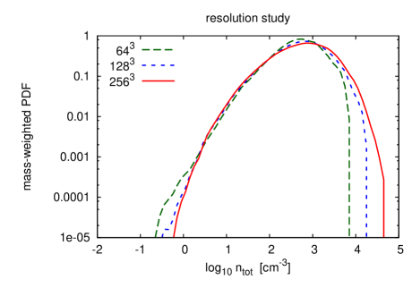
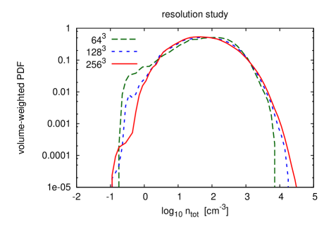
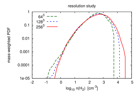
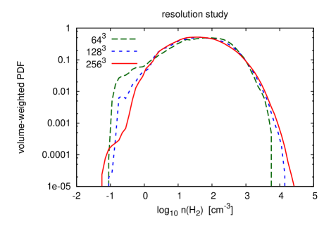
In Figure 8, we plot the mass-weighted and volume-weighted PDFs of the H₂ number density $n_{\rm H_{2}}$ at $t=t_{\rm end}$. Comparing these with the PDFs of the total number density shown in the previous Figure, we see that there is very good agreement. This is to be expected: given that only a few percent of the gas remains in atomic form at this point in the simulations, it is unsurprising that the PDF of the H₂ number density closely follows the PDF of total number density.

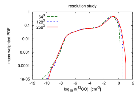
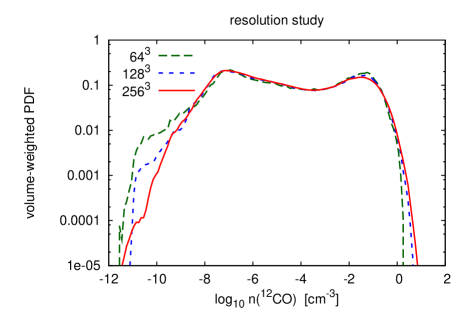
In Figure 9, we plot the mass-weighted and volume-weighted PDFs of the CO number density $n_{\rm CO}$ at $t=t_{\rm end}$. Unlike the PDFs of total number density and H₂ number density, this is not lognormal. The mass-weighted PDF has a clear peak at $n_{\rm CO}\sim 10^{-1}\>{\rm cm^{-3}}$, and falls off sharply at higher CO number densities in a fashion similar to a lognormal, but at lower CO number densities there is a clear feature in the distribution function, which decreases only slightly from $n_{\rm CO}\sim 10^{-2}\>{\rm cm^{-3}}$ down to $n_{\rm CO}\sim 10^{-8}\>{\rm cm^{-3}}$. The volume-weighted PDF also shows a peak at $n_{\rm CO}\sim 10^{-1}\>{\rm cm^{-3}}$, but is actually bimodal, with a second peak at $n_{\rm CO}\sim 10^{-7}\>{\rm cm^{-3}}$, although it is also clear that a large number of zones have CO number densities in between these two values.

The curious shape of the CO number density PDFs can be better understood once we realise that we are dealing with a PDF made up of two separate contributions, one coming from grid zones with $x_{\rm CO}\simeq x_{\rm C,tot}$ and a second from grid zones with $x_{\rm CO}\ll x_{\rm C,tot}$, and that the dependence of $n_{\rm CO}$ on $n_{\rm tot}$ is very different in these two sets of zones.

If $x_{\rm CO}\simeq x_{\rm C,tot}$, or in other words if almost all of the carbon in a zone has been converted to CO, then clearly $n_{\rm CO}$ is directly proportional to $n_{\rm tot}$. The contribution that these zones make to the PDF therefore simply mirrors the lognormal shape of the underlying mass density PDF. A significant fraction of the carbon in our simulation is located in such fully molecular zones, and it is the contribution of the gas in these regions that gives us our high density peak in the CO number density PDF.

On the other hand, if $x_{\rm CO}\ll x_{\rm C,tot}$ and, crucially, if the CO fraction is not tightly correlated with the total gas density, then we would expect to find only a weak correlation between $n_{\rm CO}$ and $n_{\rm tot}$. In other words, if the scatter in the values of $x_{\rm CO}$ in gas with a given $n_{\rm tot}$ is large, then this scatter will wash out the effects of any correlation between $n_{\rm CO}$ and $n_{\rm tot}$. As we will see later, in Section 7, a considerable fraction of the gas in our simulations behaves in this fashion, and it is this that is responsible for the extended low-density plateau that we see in the CO number density PDF. We will return to this point in Section 7.

As far as the numerical convergence of the PDFs is concerned, we see very good agreement between the results of our three runs over a very wide range of CO number densities. Differences between the three runs are only apparent in the tails of the distribution. Increasing the resolution increases the mass fraction in regions with very high CO number density, which simply reflects the fact that we better resolve the dense, post-shock gas in the highest resolution simulation, as already noted above. We also find fewer regions with very low CO number density in our higher resolution simulations, which again seems to be a consequence of the resolution-dependence of the wings of the underlying mass-density PDF.

Figure 9: (a) Mass-weighted PDF of CO number density $n_{\rm CO}$ at a time $t=t_{\rm end}$ in runs R1 (green line), R2 (blue line) and R3 (red line). (b) As (a), but for the volume-weighted PDF.

Figure 10: (a) Mass-weighted PDF of gas temperature $T$ at a time $t=t_{\rm end}$ in runs R1 (green line), R2 (blue line) and R3 (red line). (b) As (a), but for the volume-weighted PDF.

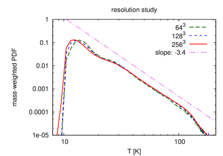
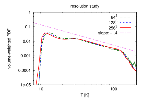
Finally, in Figure 10, we plot the mass-weighted and volume-weighted PDFs of the gas temperature $T$ at $t=t_{\rm end}$. Several features of these plots stand out. First, as the temperature approaches 10 K, the PDF falls steeply, and there is almost no gas in the simulation with $T<10\>{\rm K}$. This feature of the plot is artificial, and is a consequence of our adoption of a temperature floor at $T=T_{\rm dust}=10\>{\rm K}$ in our treatment of the radiative cooling (see §2.3.2 above). Thus, the only fluid elements that have $T<10\>{\rm K}$ are those that had temperatures close to 10 K and then underwent a strong rarefaction, leading to significant adiabatic cooling. Moreover, this must have happened within the last 0.1 Myr, or else cosmic ray heating would have warmed the gas up above 10 K again. As is apparent from the PDFs, very few of the fluid elements in our simulations find themselves in this situation at any given time.

The second obvious feature of the temperature PDFs is the clear power-law tail between 30 K and 120 K in both the mass and the volume-weighted PDFs. This tail is composed of gas with a low $A_{\rm V,eff}$ that is heated primarily by photoelectric emission from dust grains and is cooled primarily by C⁺ fine structure emission. The equilibrium temperature of this gas varies approximately as a power-law function of density, $T_{\rm eq}\propto n^{0.7}$ (Larson, 2005; Glover & Mac Low, 2007b).

Regarding numerical convergence, we again find good convergence for the majority of the PDF, with significant differences visible only around the low temperature peak in the distribution. Increasing the numerical resolution shifts the peak to slightly lower gas temperatures, reflecting the fact that the coldest gas is also, typically, the densest, and that this dense material is better resolved in the higher resolution simulations.

6.2 Time evolution of the PDFs

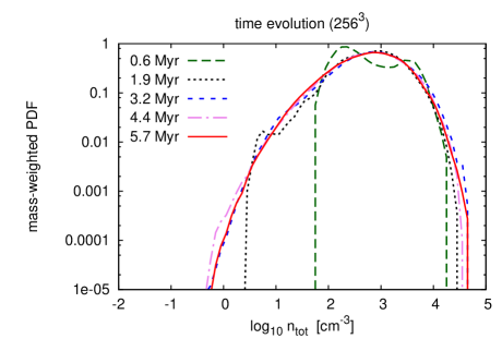
In Figure 11a, we show how the mass-weighted PDF of the total number density evolves with time in the $256^{3}$ run R3. The first output time for which data is plotted, $t=0.6\>{\rm Myr}$, corresponds to less than half of a turbulent crossing time, and at this point in the simulation, the imprint of the initial conditions is still quite apparent. The density PDF at this time is clearly not lognormal. Instead, it is bimodal, with one peak close to the starting density $n_{0}=300\>{\rm cm^{-3}}$, corresponding to gas which has not yet been significantly affected by the turbulence, and a second peak at $n\sim 3000\>{\rm cm^{-3}}$, corresponding to gas that has already been compressed by the strong, large-scale shocks present in the initial turbulent velocity field.

By the time of the second output dump at $t=1.9\>{\rm Myr}$, corresponding to roughly one turbulent crossing time, the picture is quite different. The characteristic lognormal density PDF has now been established, although a few fluctuations in the low density tail of the PDF are still apparent. These have vanished by the time of our third output dump, at $t=3.2\>{\rm Myr}$, and from this point on we see very little evidence for any change in the PDF, suggesting that the density distribution has reached a statistical steady state.

Figure 11: (a) Evolution with time of the mass-weighted PDF of the total number density $n_{\rm tot}$ in our $256^{3}$ zone run, R3. Values are plotted for $t=0.6\>{\rm Myr}$ (green long-dashed line), $t=1.9\>{\rm Myr}$ (black dotted line), $t=3.2\>{\rm Myr}$ (blue short-dashed line), $t=4.4\>{\rm Myr}$ (mauve dot-dashed line) and $t=5.7\>{\rm Myr}$ (red solid line). (b) As (a), but for the ${\rm H_{2}}$ number density. (c) As (a), but for the CO number density. (d) As (a), but for the gas temperature.

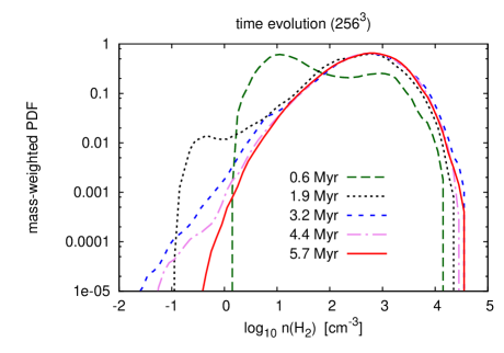
In Figure 11b, we plot the mass-weighted PDF of the H₂ number density in run R3 at various output times. As in Figure 11a, the PDF at the earliest output time is clearly not lognormal, but after one turbulent crossing time, it has become lognormal over much of the range of densities plotted. This is easily understood when one considers that by $t=1.9\>{\rm Myr}$, roughly 80% of the hydrogen in the simulation has already become molecular (see Figure 4) and that we expect there to be a clear correlation between gas density and molecular fraction (see Glover & Mac Low 2007b, or §7 below). At gas densities where the hydrogen is almost fully molecular, we expect that the H₂ number density PDF will simply track the underlying density PDF. Comparison of Figures 11a and 11b shows that this is the case for H₂ number densities greater than $n_{\rm H_{2}}\sim 10\>{\rm cm^{-3}}$ at $t=1.9\>{\rm Myr}$. Lower H₂ number densities correspond to regions of low density gas where a significant fraction of atomic hydrogen remains, and in these regions there is no simple mapping between gas density and H₂ number density, since here the H₂ fraction is sensitive not only to the current density and the degree of shielding, but also to the previous dynamical history of the gas (Glover & Mac Low, 2007b; Federrath et al., 2008). It is therefore not surprising that at these low densities the PDF is not lognormal.

At later output times, we see little change in the PDF at densities $n_{\rm H_{2}}>10\>{\rm cm^{-3}}$, which simply reflects the fact that there is very little change in the underlying density PDF. At lower densities, the PDF continues to evolve with time. The mass fraction of gas with extremely low H₂ number densities, $n_{\rm H_{2}}<0.3\>{\rm cm^{-3}}$, significantly decreases. This gas physically corresponds to gas with a low total number density and low H₂ fraction. As time passes, the H₂ fraction in this gas increases, and so the H₂ number densities increase, even though the statistical distribution of the total number densities is unchanged. At the latest output time, $t=5.7\>{\rm Myr}$, the shape of the full H₂ number density PDF is almost identical to that of the full density PDF, since by this point, almost all of the hydrogen has become molecular.

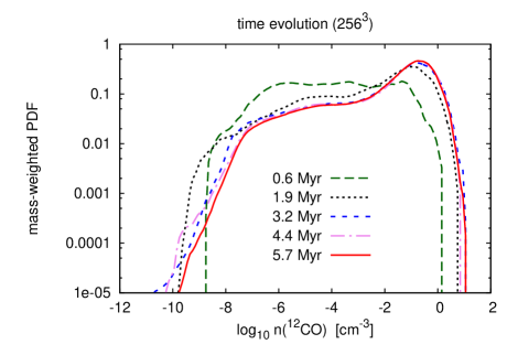
In Figure 11c, we show how the mass-weighted PDF of the CO number density evolves with time in run R3. Just as with $n_{\rm tot}$ and $n_{\rm H_{2}}$, the shape of the PDF at our earliest output time bears little resemblance to its later shape, while by the time of the second output dump, the shape of the final PDF has become far better established. Unlike $n_{\rm tot}$ and $n_{\rm H_{2}}$, however, we continue to see evolution in both the low and the high density portions of the PDF, and it is only after $3.2\>{\rm Myr}$, corresponding to 1.6 turbulent crossing times, that the CO number density PDF reaches a statistical steady state. This longer evolutionary timescale is a consequence of the longer time required to form CO, compared to H₂. Between $t=1.9\>{\rm Myr}$ and $t=3.2\>{\rm Myr}$, the total mass of H₂ in the simulation increases by about 15%, while the total mass of CO increases by about 50%.

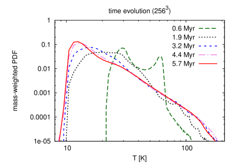
Finally, in Figure 11d, we show how the mass-weighted temperature PDF varies with time. At the earliest output time, this has a two-peaked structure: a high temperature peak, centered on $T\sim 65\>{\rm K}$, corresponding to unshocked gas that still has a density and temperature close to its initial value, and a low temperature peak, centered on $T\sim 30\>{\rm K}$, corresponding to shocked, higher-density gas (compare with the density PDF at $t=0.6\>{\rm Myr}$ in Figure 11a). By $t=1.9\>{\rm Myr}$, this double-peaked structure has disappeared, but as with the CO number density PDF, it is not until $t=3.2\>{\rm Myr}$ that large portions of the PDF settle into their final form. By this point, the power-law high temperature tail has become fully established, and the PDF at temperatures $T>30\>{\rm K}$ shows very little evolution at later times. On the other hand, the portion of the PDF around the low temperature peak continues to evolve. The PDF peaks at $T\simeq 16\>{\rm K}$ at $t=3.2\>{\rm Myr}$, but by $t=4.4\>{\rm Myr}$ the peak has shifted to $T\simeq 13\>{\rm K}$, while by $t=5.7\>{\rm Myr}$, it has shifted further, to $T\simeq 12\>{\rm K}$. We therefore see a systematic increase with time of the amount of cold gas present in the simulation. This increase has not yet come to an end by the end of our simulation, although it has significantly slowed: there is far more evolution in the temperature PDF between $t=3.2\>{\rm Myr}$ and $t=4.4\>{\rm Myr}$ than there is between $t=4.4\>{\rm Myr}$ and $t=5.7\>{\rm Myr}$. This increase in the mass of cold gas is simply driven by radiative cooling of dense, fully-molecular gas. At temperatures $T\gg 10\>{\rm K}$, the cooling time of the gas is very short, but for temperatures close to our temperature floor of 10 K, it becomes comparable to the dynamical time (see e.g. Figure 2a in Neufeld, Lepp & Melnick, 1995).

7 Spatial distribution of $\mathbf{H_{2}}$ and CO

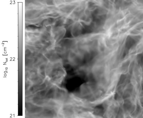
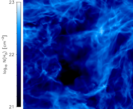
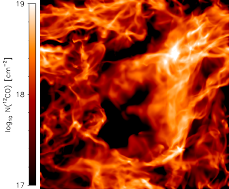
In Figure 12a, we plot the column density of hydrogen nuclei, $N_{\rm H,tot}$, projected along the $z$-axis of the simulation (i.e. along the axis parallel to the direction of the initial magnetic field) in run R3 and at time $t=t_{\rm end}$. In Figures 12b and 12c, we show similar plots of the H₂ and CO column densities. The basic morphology of the gas is the same in all three plots. The gas has a filamentary distribution, and large spatial variations in the column densities are apparent, including, coincidentally, a rather prominent under-density visible toward the bottom-left of the figures. The plots of $N_{\rm H,tot}$ and $N_{\rm H_{2}}$ are very difficult to distinguish, which is unsurprising since most of the hydrogen gas in the simulation is molecular by this point. On the other hand, the plot of CO column density is clearly different from the other two plots: the underdense regions are larger, and also more numerous, particularly towards the edges of the box. Similar results are found if we consider projections along lines of sight perpendicular to the initial magnetic field.

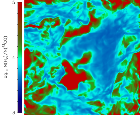
The difference between the spatial distributions of $N_{\rm CO}$ and $N_{\rm H_{2}}$ can be more clearly highlighted by plotting the ratio $N_{\rm H_{2}}/N_{\rm CO}$, as we do in Figure 12d. Along lines of sight corresponding to the highest column densities, this ratio is around $10^{3.5}$, as we would expect for gas in which all of the hydrogen is in the form of H₂ and all of the carbon is in the form of CO. However, if we look along lines of sight that pass through regions of lower total column density, then we find values for this ratio that are up to a factor of thirty larger. Along these lines of sight, much of the carbon remains in the form of C or C⁺. It is clear from Figure 12d that the regions with low CO column densities are found preferentially towards the edges of the simulation volume. This is only to be expected, given our treatment of the external ultraviolet radiation. Gas close to an edge of the simulation volume will tend to have a low column density of dust between itself and the edge, and so will be more readily affected by UV photons propagating inwards in that direction, even if in other directions, that same gas is well-shielded. However, it should be stressed that this is not simply an edge effect: when the column density is low, UV photons can penetrate in to the volume to considerable depths, and are not confined to a narrow region at the surface of the box.

Similarly, the two large regions with high H₂:CO column density ratios that are close to the center of the projections are well-shielded by dust along the $x$ and $y$ axes of the simulation, but have a low column density of material shielding them in the $z$ direction, and so are strongly affected by UV photons propagating inwards in that direction.

Clearly, if we were to solve for the UV radiation field using much higher angular resolution, we would expect to obtain slightly different results for the spatial distributions of the CO column density and the H₂:CO column density ratio. Nevertheless, the picture we obtain here is qualitatively correct. The clumpiness created by the turbulence opens up channels in the gas distribution, allowing UV photons to propagate far deeper into the cloud than would be possible if it were a single homogeneous mass of gas (see also Boisse, 1990; Padoan et al., 2004; Bethell, Zweibel & Li, 2007).

Figure 12: (a) Column density of hydrogen nuclei, $N_{\rm H,tot}$, in run R3 at time $t=t_{\rm end}$, viewed along a line of sight parallel to the $z$-axis of the simulation volume. This direction is also parallel to the initial orientation of the magnetic field. (b) As (a), but for the ${\rm H_{2}}$ column density. (c) As (a), but for the CO column density. (d) Ratio of ${\rm H_{2}}$ column density to CO column density along the same line of sight through run R3 at time $t=t_{\rm end}$.

7.1 CO to $\mathbf{H_{2}}$ ratio

The results shown in Figure 12 indicate that the amount of CO in the gas depends in part upon the column density of the material shielding the gas, but being two-dimensional projections, they do not easily allow us to quantify this dependence, or to separate the effects of increased shielding from the effects of increased gas number density. To do this, we need to make use of the full three-dimensional spatial information contained in the datacube.

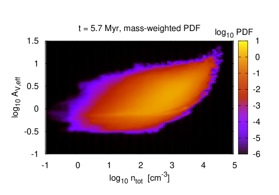
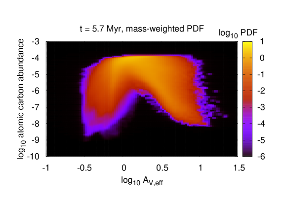
In Figure 13a, we show how the fractional abundance of CO, $x_{\rm CO}$, depends on the number density $n_{\rm tot}$ by plotting the mass-weighted two-dimensional PDF of these two quantities. In Figure 13b, we show a similar plot of $x_{\rm CO}$ versus the effective visual extinction $A_{\rm V,eff}$. For a grid cell at position $\vec{x}$, we define the effective visual extinction $A_{\rm V,eff}$ as

$$A_{\rm V,eff}=-\frac{1}{2.5}\ln\left[\frac{1}{6}\left(\sum_{p=1}^{3}e^{-2.5A_{\rm V}(x_{p+})}+e^{-2.5A_{\rm V}(x_{p-})}\right)\right]$$ (29)

where $A_{\rm V}(x_{p+})$ is the visual extinction of material between the cell and the edge of the volume in the positive direction along the $x_{p}$ axis, and $A_{\rm V}(x_{p-})$ is the same in the negative direction. The choice of the factor of 2.5 occurs because the CO photodissociation rate scales with the visual extinction $A_{\rm V}$ as $\exp(-2.5A_{\rm V})$. The value of $A_{\rm V,eff}$ corresponds to the visual extinction used in our code, in the context of our six-ray approximation, for computing the CO photodissociation rate (see Section 2.2).

Figure 13: (a) Mass-weighted two-dimensional PDF of CO fractional abundance $x_{\rm CO}$ versus gas number density $n_{\rm tot}$. (b) Mass-weighted two-dimensional PDF of CO fractional abundance $x_{\rm CO}$ versus effective visual extinction $A_{\rm V,eff}$ (defined in Equation 29). (c) Mass-weighted two-dimensional PDF of $x_{\rm CO}$ versus $\exp(+2.5A_{\rm V,eff})n_{\rm tot}$. (d) Mass-weighted two-dimensional PDF of $x_{\rm CO}$ versus $\xi$, defined in Equation 34.

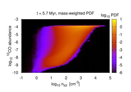
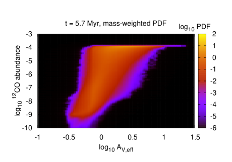
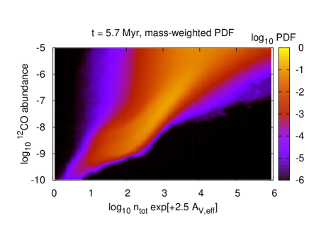
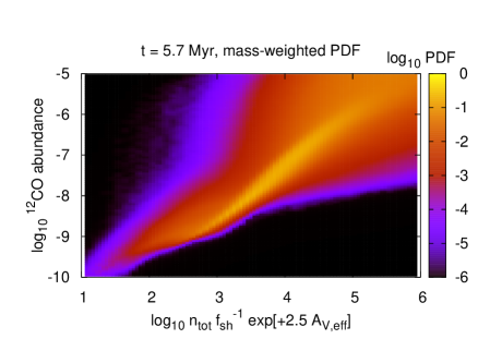
Figure 13a demonstrates that there is only a weak correlation between the CO abundance and the number density. At densities $n_{\rm tot}<10\>{\rm cm^{-3}}$, most of the gas has a very low CO abundance, $x_{\rm CO}<10^{-8}$. On the other hand, at densities $n_{\rm tot}>10^{4}\>{\rm cm^{-3}}$, almost all of the carbon in the gas is found in the form of CO. At densities between these two extremes, however, there is a very wide spread in $x_{\rm CO}$ at any given $n_{\rm tot}$. For instance, at $n_{\rm tot}=100\>{\rm cm^{-3}}$, values of $x_{\rm CO}$ between $10^{-9}$ and $1.4\times 10^{-4}$ are almost equally probable. This large scatter in $x_{\rm CO}$ is unexpected and demands an explanation.

A large part of the puzzle is explained by Figure 13b, which shows that there is a correlation between $x_{\rm CO}$ and the effective visual extinction, $A_{\rm V,eff}$, that is stronger than the correlation between CO fraction and gas number density. This is in line with our expectations based on our discussion of the H₂:CO column density ratio above, and is also readily explained by considering the microphysics of CO formation and destruction. Consider the following simplified model for the CO abundance. CO is formed from gas phase C or C⁺ by a variety of reactions, but the most important ones involve either a hydrocarbon radical (e.g. CH) or its ion (e.g. CH⁺), or the OH radical or its ion, OH⁺. In cold gas, the formation of one of these intermediate species is the rate-limiting step in forming CO, as the various routes by which these species can be formed typically involve either a radiative association reaction with H₂, or the cosmic ray ionization of H₂, both of which are slow processes. Let us suppose, for simplicity, that reactions involving hydrocarbon radicals and ions dominate. In that case, we can write the CO formation rate as $R_{\rm form}n_{\rm C,tot}n_{\rm H_{2}}$, where $n_{\rm C,tot}=n_{\rm C}+n_{\rm C^{+}}$, and where $R_{\rm form}$ is the formation rate of our intermediate species, multiplied by a factor that accounts for the fact that some of the intermediate radicals and ions will be photodissociated, rather than reacting to form CO (or a further intermediate, such as CO⁺, that reacts rapidly to form CO). If CO is primarily destroyed by photodissociation, at a rate $R_{\rm pd}n_{\rm CO}$, then in chemical equilibrium, the CO fractional abundance is given by

$$x_{\rm CO}=\left(\frac{R_{\rm form}}{R_{\rm pd}}\right)x_{\rm C,tot}n_{\rm H_{2}}.$$ (30)

The photodissociation rate $R_{\rm pd}$ can be written in terms of $A_{\rm V,eff}$ as $R_{\rm pd}=2\times 10^{-10}f_{\rm sh}\exp(-2.5A_{\rm V,eff})$, where $f_{\rm sh}=f_{\rm CO}f_{\rm H_{2}}$ is the product of the shielding factors due to CO self-shielding ($f_{\rm CO}$) and due to the shielding of CO by H₂ ($f_{\rm H_{2}}$) that we introduced in §2.2. We can therefore rewrite Equation 30 as

$$x_{\rm CO}=\left(\frac{R_{\rm form}}{2\times 10^{-10}}\right)f_{\rm sh}^{-1}e^{2.5A_{\rm V,eff}}x_{\rm C,tot}n_{\rm H_{2}}.$$ (31)

Consideration of the different processes involving C or C⁺ that lead to the formation of CH or CH⁺ suggests that $R_{\rm form}$ should have a value of roughly $10^{-17}\>{\rm cm^{3}}\>{\rm s^{-1}}$, give or take an order of magnitude. If we assume, again for simplicity, that in fact $R_{\rm form}=2\times 10^{-17}\>{\rm cm^{3}\>s^{-1}}$, then Equation 31 becomes

$$x_{\rm CO}=10^{-7}e^{2.5A_{\rm V,eff}}f_{\rm sh}^{-1}x_{\rm C,tot}n_{\rm H_{2}}.$$ (32)

If we further simplify matters by assuming that the H₂ fraction is of order one, and that most of the carbon in the gas is still in the form of C or C⁺, so that $x_{\rm C,tot}\sim 10^{-4}$, then we obtain the following expression for $x_{\rm CO}$

$$x_{\rm CO}\sim 10^{-11}e^{2.5A_{\rm V,eff}}f_{\rm sh}^{-1}n.$$ (33)

Given the large number of assumptions and simplifications that we have made above, this expression should clearly be treated only as a rough order-of-magnitude estimate of the CO abundance. Nevertheless, this simplified model does highlight some of the behaviour that we see for the actual CO abundance in our simulations. Our simplified model predicts that the abundance of CO should vary only linearly with the gas number density, and with $f_{\rm sh}^{-1}$ (which itself is a complicated function of $N_{\rm H_{2}}$ and $N_{\rm CO}$), but should vary exponentially with $A_{\rm V,eff}$. Thus, small changes in $A_{\rm V,eff}$ will produce a much larger change in $x_{\rm CO}$ than even relatively large changes in $n$, and so we would expect to find a much stronger correlation between $x_{\rm CO}$ and $A_{\rm V,eff}$ than between $x_{\rm CO}$ and $n_{\rm tot}$, as indeed is the case in our simulations (see Figure 13).

Figure 14: Mass-weighted two-dimensional PDF of $A_{\rm V,eff}$ versus $n_{\rm tot}$.

If the behaviour of $x_{\rm CO}$ is determined primarily by the amount of shielding by dust and molecules, rather than by the density, then we would expect to obtain a much tighter correlation if, instead of plotting $x_{\rm CO}$ against $n_{\rm tot}$, we plot $x_{\rm CO}$ against $n_{\rm tot}\exp(2.5A_{\rm V,eff})$ or, even better, against

$$\xi\equiv n_{\rm tot}\exp(2.5A_{\rm V,eff})f_{\rm sh}^{-1}.$$ (34)

This we have done in Figures 13c and 13d. These Figures show that when the CO fraction is small, then we obtain a much tighter correlation between $x_{\rm CO}$ and $\xi$ than between $x_{\rm CO}$ and $n_{\rm tot}$, while accounting for the effects of shielding from CO and H₂ improves the correlation even further. This confirms that most of the scatter we see in the $x_{\rm CO}$–$n_{\rm tot}$ plot at low $x_{\rm CO}$ is due to the fact that the CO fraction is far more sensitive to changes in the amount of shielding than to changes in the density, and that the amount of shielding is not well correlated with the gas density. This point is further emphasised in Figure 14, which shows that there is indeed a large scatter in the effective visual extinction at most densities.

If the CO abundance is large, then the relationship between $x_{\rm CO}$ and the amount of shielding becomes quite different, and the clear correlation found at low $x_{\rm CO}$ rapidly vanishes. Our simplified model for $x_{\rm CO}$ again can give us insight into why this happens. Consider that in order to produce a CO abundance $x_{\rm CO}\sim 10^{-5}$, our model predicts that we must have $\xi\sim 10^{6}$. For a gas density $n\sim 300\>{\rm cm^{-3}}$, this means that the CO photodissociation rate is reduced by a factor of roughly 3000 compared to the optically thin value, i.e. $R_{\rm pd}\sim 10^{-13}\>{\rm s^{-1}}$. The corresponding photodissociation timescale is then $0.3\>{\rm Myr}$, which is not negligible in comparison to the dynamical timescale of the gas, and so it is probably no longer safe to assume either that the gas is in chemical equilibrium or that photodissociation dominates the destruction of CO. As our model was based on both of these assumptions, it is unsurprising that it breaks down at high $x_{\rm CO}$.

To summarise, what these results are showing us is that in low extinction gas, the CO abundance is determined by a combination of the extinction and the density, with the extinction playing the primary role, while at high extinction, other physics, such as the dynamical history of the gas, or the impact of other destruction mechanisms, such as charge transfer with $\rm{He}^{+}$, becomes far more important.

The relationship between $A_{\rm V,eff}$ and $n_{\rm tot}$, shown in Figure 14, is also worth discussing. As noted above, there is no strong correlation between these two quantities. However, they are not completely uncorrelated either. There is a clear deficit of zones with high $A_{\rm V,eff}$ at low densities, and there is also a deficit of zones with low $A_{\rm V,eff}$ at high densities. The latter is a consequence of the finite resolution of our simulation, since the value of $A_{\rm V,eff}$ in a given zone has a lower bound

$$A_{\rm V,eff}=\frac{0.5n\Delta x}{1.87\times 10^{21}\>{\rm cm^{-2}}},$$ (35)

where $\Delta x$ is the size of a grid zone, corresponding to absorption within the zone itself. However, this does not explain the deficit of points with high extinction and low density. Instead, this is due to the fact that there are only very few voids in the density distribution that are entirely surrounded by high extinction material. In addition, little of the mass in the simulation volume is to be found at these very low densities.

Also of interest is the fact that the smallest values of $A_{\rm V,eff}$ found in our simulation are roughly 0.1–0.3, rather than zero. The reason for this is quite simple. The regions in the simulation with the lowest values of $A_{\rm V,eff}$ are those at the edges and corners. These regions are highly exposed to radiation propagating inwards from the nearest edges of the box. However, at the same time, they are very well shielded from radiation propagating inwards from the opposite edges of the box, since they are protected by the full width of gas in the simulation. Therefore, these zones see a mean intensity that is smaller than the mean intensity that they would see if the opacity in every direction were zero, and hence they have a non-zero $A_{\rm V,eff}$, even though the visual extinction between them and the closest edge of the box may be very close to zero. It is also clear that our “six-ray” approximation tends to overestimate the degree to which the zones at the edges of the box are shielded. For instance, consider a zone located at the edge of the box, in the center of one of the six faces. In one direction it has a very low $A_{\rm V}$; however, in the other five directions, it may have a very high $A_{\rm V}$. Therefore, using our approximation we would predict that it would see a mean intensity of radiation that was roughly one-sixth of the value in the absence of shielding, while in reality it should see a mean intensity that is only one-half of the optically thin value. Fortunately, this is only really a problem for zones right at the edge of our simulation, and most of the gas should not be significantly affected. To test this, we verified that the removal of 32 zones of material from each of the edges of our $256^{3}$ simulation did not significantly affect the PDFs reported in this paper.

Figure 15: Mass-weighted two-dimensional PDF of the fractional abundance of atomic carbon, $x_{\rm C}$ versus effective visual extinction $A_{\rm V,eff}$.

7.2 Comparison to photodissociation region models

To conclude this section, it is interesting to compare our results for the CO distribution with what we would expect based on classical models of uniform density photodissociation regions (see e.g. Hollenbach & Tielens, 1999, and references therein). These predict that we should find an outer shell of C⁺ surrounding a shell of neutral carbon, that in turn surrounds a central region dominated by CO. If we examine how the C and CO abundances vary with visual extinction (Figures 13b and 15), then they are to some degree consistent with this picture. We see a peak in the typical atomic carbon abundance at $A_{\rm V,eff}\sim 1$, followed by a decline at higher $A_{\rm V,eff}$, as CO begins to dominate. However, what is apparent in both figures is the large degree of scatter around this underlying trend. There are many regions of high extinction in which the C abundance is very small, as the PDR models would predict, but at the same time there are also regions in which $x_{\rm C}$ remains large at high $A_{\rm V}$. Similarly, although most regions with $A_{\rm V}>2$ are CO dominated, there is also a significant amount of mass with high extinction that still has a very low CO abundance.

Some of this scatter is surely due to the highly inhomogeneous nature of the density field. As we have already seen, the density of gas with a given $A_{\rm V,eff}$ can vary over several orders of magnitude. In addition, it is likely that turbulent mixing of material between high extinction and low extinction sightlines also plays an important role in determining the spatial distribution of C⁺, C and CO (see also Glover & Mac Low, 2007b; Federrath et al., 2008). To properly disentangle these effects lies beyond the scope of this introductory paper, but is something we plan to revisit in future work.

8 Summary

In this paper, we have outlined the methods that we have developed to model the coupled thermal, chemical and dynamical evolution of the turbulent gas making up giant molecular clouds. We have shown that it is now possible to perform high-resolution simulations in three dimensions that track the thermal and chemical evolution of the gas in a realistic fashion. The chemical network that we use in our simulations is significantly simplified compared to the most detailed models available, but nevertheless performs with acceptable accuracy for our purposes, and the largest errors in our models come not from our simplified chemistry, but from our approximate treatment of the effects of the external radiation field.

We have performed simulations with numerical resolutions of $64^{3}$, $128^{3}$ and $256^{3}$, and have demonstrated that most of our results are well-converged in our $256^{3}$ run. The main exception is the high density tail of the density PDF, which is not fully converged at a resolution of $256^{3}$ zones (although the peak of the density PDF is well converged). This results from the improvement of our ability to resolve dense post-shock gas with increasing numerical resolution, and is also responsible for the small dependence on resolution that remains in our determination of the O₂ and H₂O abundances, and in the gas temperature distribution at the lowest temperatures.

We have also quantified the timescales on which various quantities of interest reach a statistical steady state. The density PDF, which has the same log-normal form as found in many previous simulations of interstellar turbulence, reaches a steady state after roughly one and a half turbulent crossing times, as does the H₂ number density distribution in all but the lowest density gas. On the other hand, the CO number density distribution takes closer to two crossing times to settle into a steady state, and the temperature distribution still has not reached a final steady state after three crossing times.

We find that CO formation occurs rapidly in the dense, turbulent gas studied here. Most of the CO is produced within the first 2–3 Myr of the simulation, i.e. within 1–2 turbulent crossing times. For comparison, most of the H₂ produced in the simulation forms within a single crossing time. These short chemical timescales suggest that the limiting timescale in the formation of a molecular cloud is not the time required to convert the hydrogen to H₂ and the carbon to CO, but rather the time required to assemble the cloud material from the low density ISM. Once large enough spatial and column densities are reached, conversion of the gas to molecular form should follow very quickly.

Our simulations also demonstrate that the gas in molecular clouds is not isothermal. Most of the molecular gas has a low temperature, in the range of 10–20 K, but there is also a clear power-law tail in the temperature PDF at higher temperatures, made up of low extinction gas heated by photoelectric emission from dust grains.

We have found that the CO abundances produced in our simulations are not well correlated with the gas density. This means that the use of a density cut to identify molecular regions in turbulence simulations that do not self-consistently follow the chemical evolution of the gas is dangerous, and may give misleading results. Similarly, the assumption that all observed CO is at roughly the same gas density may be similarly misleading, as is the assumption that all of the CO in a molecular cloud is located at densities that are high enough for its rotational lines to be thermalized.

The poor correlation that we find between CO abundance and gas density is explained by the sensitivity of the CO to the amount of UV shielding provided by the dust, H₂ and CO. Variations in the amount of shielding produce a far greater variation in the CO abundance than do variations in the gas density. In addition, the amount of shielding provided by the gas is not well correlated with the density, owing to the highly inhomogeneous nature of the density field. The important role that density inhomogeneities play in determining the chemical structure of molecular clouds has long been recognized (see e.g. Stutzki & Guesten, 1990; Gierens, Stutzki & Winnewisser, 1992; Williams, Blitz & Stark, 1995), but the most sophisticated current PDR models continue to rely on a somewhat artificial picture of their structure, visualising them as an ensemble of clumps with well-defined densities surrounded by a much lower density interclump medium (e.g. Sun et al., 2008; Kramer et al., 2008). The picture suggested by our simulations is rather different. We find a continuous density distribution, with no clear separation between ‘clump’ and ‘interclump’ material, and with continual turbulent mixing of gas between low-density and high-density regions. We look forward to exploring the observational consequences of this picture in greater detail in future work.

Appendix A Ensuring consistent advection of chemical species

A.1 Consistent Multi-fluid Advection (CMA)

Let $x_{m}(i,j,k)$ be the fractional abundance relative to hydrogen of chemical species $m$ in grid zone $(i,j,k)$, let $X_{n}(i,j,k)$ be the elemental abundance, relative to hydrogen, of element $n={\rm H},{\rm He},{\rm C}$ or O in grid zone $(i,j,k)$, and let $N_{n,m}$ be the number of nuclei of element $n$ in species $m$. Then for each element $n$, we can construct a constraint equation of the form

$$\sum_{m}N_{n,m}x_{m}(i,j,k)=X_{n}(i,j,k).$$ (36)

Now, if we assume that the elemental composition of the gas remains the same throughout our simulation volume, i.e. that the elemental abundances $X_{n}$ are independent of position, then these constraint equations become

$$\sum_{m}N_{n,m}x_{m}(i,j,k)=X_{n}.$$ (37)

Although it is trivial to ensure that these constraints are satisfied at the start of our simulations, ensuring that they remain satisfied as the gas is evolved forward in time is not so simple.

The root cause of the problem is to be found in the advection scheme. Most Eulerian treatments of multi-species flows model the species abundances $x_{m}$ as passive scalars that are advected with the flow. If we consider a one-dimensional scheme, for simplicity, then we can write the advection equation for a given species $m$ in grid zone $i$ in finite volume form as

$$\rho_{i}x_{m,i}(t+\Delta t)\Delta V_{i}=\rho_{i}x_{m,i}(t)\Delta V_{i}-\Delta t\left[A_{i+1/2}F_{i+1/2}-A_{i-1/2}F_{i-1/2}\right],$$ (38)

where $F_{i+1/2}=\rho_{i+1/2}v_{i+1/2}x_{m,i+1/2}$ is the flux of $x_{m}$ from zone $i$ into zone $i+1$, $F_{i-1/2}=\rho_{i-1/2}v_{i-1/2}x_{m,i-1/2}$ is the flux of $x_{m}$ from zone $i-1$ into zone $i$, $A_{i-1/2}$ and $A_{i+1/2}$ are the areas of the interfaces between zones $i-1$ and $i$, and between zones $i$ and $i+1$, respectively, and $\Delta V_{i}$ is the zone volume.

If the elemental abundances $X_{n}$ are independent of position, then at both interfaces of zone $i$, the species fluxes should satisfy the constraint equations

$$\left[\sum_{m}N_{n,m}x_{m,i\pm 1/2}\right]\rho_{i\pm 1/2}v_{i\pm 1/2}=X_{n}\rho_{i\pm 1/2}v_{i\pm 1/2}.$$ (39)

In order to ensure stability, fluxes are often computed from the distribution of the flow variables upstream of the interface (“upwinding”) using some interpolation scheme. For instance, in ZEUS-MP, which uses van Leer (1977) advection, the upwinded interpolated value $q_{i}^{*}$ of a zone-centered scalar $q$ at the negative interface of zone $i$ is given by (Stone & Norman, 1992a)

$$q_{i}^{*}=\left\{\begin{array}[]{lr}q_{i-1}+(\Delta x_{i-1}-v_{i-1/2}\Delta t)(dq_{i-1}/2)&\hskip 36.135ptv_{i-1/2}>0\\ q_{i}+(\Delta x_{i}+v_{i-1/2}\Delta t)(dq_{i}/2)&\hskip 36.135ptv_{i-1/2}<0\end{array}\right.$$ (40)

where $q_{i}$ is the zone-centered value of $q$ in zone $i$, $\Delta x_{i}$ is the size of zone $i$, and $dq_{i}$ is the monotonized van Leer slope, given by

$$dq_{i}=\left\{\begin{array}[]{lr}\frac{2(\Delta q_{i-1/2}\Delta q_{i+1/2})}{\Delta q_{i-1/2}+\Delta q_{i+1/2}}&\hskip 36.135pt\Delta q_{i+1/2}\Delta q_{i-1/2}>0\\ 0&\hskip 36.135pt\Delta q_{i+1/2}\Delta q_{i-1/2}\leq 0\end{array}\right.$$ (41)

where $\Delta q_{i+1/2}=(q_{i+1}-q_{i})/\Delta x_{i}$. (Note that in Equation 40, we have neglected any motion of the underlying coordinate grid, for simplicity). Given $q_{i}^{*}$, the flux then follows from $F_{i-1/2}=q_{i}^{*}v_{i-1/2}$. Also in common usage is the Piecewise Parabolic Method (PPM) of Colella & Woodward (1984), which uses higher-order interpolation, and so produces a better quality solution (at the cost of increased computational effort).

Unfortunately, as several authors have noted (Fryxell, Müller & Arnett, 1989; Larrouturou, 1991; Plewa & Müller, 1999), the fact that the interpolation profiles in these schemes are constructed independently for each chemical species means that there is no guarantee that the resulting fluxes actually satisfy Eq. 39. In general, they do not do so. Moreover, this violation occurs even when the underlying advection scheme is conservative. Thus, even if our initial chemical abundances satisfy the constraints represented by Equation 37, as soon as we begin advecting them with a standard higher-order scheme, these constraints will be violated.

This problem is often dealt with by a renormalization of species abundances following the advection step to ensure that Eq. 37 is satisfied. However, as Plewa & Müller (1999) note, this procedure lacks any formal justification and can lead to large systematic errors in the abundances of the least abundant species. It can also destroy the conservative nature of the scheme. Plewa & Müller (1999) suggest an improved way of dealing with this problem, which they term the Consistent Multi-fluid Advection (CMA) method. They consider the case in which one has only a single constraint equation

$$\sum_{m}N_{1,m}x_{m}(i,j,k)=1,$$ (42)

where we have chosen to set $X_{n}=1$ for simplicity. The example they consider is a fluid consisting of many different elements (but no composite molecules), whose mass fractions must sum to unity. An alternative example, more in keeping with our discussion here, is a gas consisting of only one element (e.g. hydrogen) that can form several different stable chemical species (e.g. $\rm{H}^{+}$, ${\rm H^{-}}$, ${\rm H}$, ${\rm H_{2}}$). They show that in this case, one can satisfy Equation 42 while preserving the conservative nature of the advection scheme by replacing the interpolated abundances $x_{i\pm 1/2,m}$ used to construct the fluxes in Equation 38 with the modified abundances

$$\chi_{i\pm 1/2,m}=\frac{x_{i\pm 1/2,m}}{\sum_{m}N_{1,m}x_{i\pm 1/2,m}}.$$ (43)

In other words, instead of ensuring that the constraint equation is satisfied by normalizing the abundances after the advection step, we ensure that it is satisfied by normalizing the fluxes during the advection step.

When dealing with the PPM code, additional modifications are necessary to avoid problems related to PPM’s contact discontinuity detection algorithm, as discussed in Section 2.3 of Plewa & Müller (1999). However, these problems do not occur with the simpler van Leer advection scheme used in ZEUS-MP, and so we do not discuss them further here.

A.2 Extending the CMA algorithm

Although Plewa & Müller’s CMA algorithm is simple to implement and is highly effective in practice, its applicability to chemically reacting flow is limited. The problem comes from the assumption that the chemical abundances must satisfy only a single constraint equation. In a flow containing compounds of multiple elements, such as CO, this is not the case. In such a flow, our modified interface abundances for carbon and oxygen must satisfy both

$$\sum_{m}N_{{\rm C},m}x_{m}=X_{\rm C}$$ (44)

and

$$\sum_{m}N_{{\rm O},m}x_{m}=X_{\rm O}$$ (45)

If we rescale the abundances of those species containing carbon according to

$$\chi_{i\pm 1/2,m}=\frac{X_{\rm C}}{\sum_{m}N_{{\rm C},m}x_{i\pm 1/2,m}}x_{i\pm 1/2,m}$$ (46)

and those species containing oxygen according to

$$\chi_{i\pm 1/2,m}^{\prime}=\frac{X_{\rm O}}{\sum_{m}N_{{\rm O},m}x_{i\pm 1/2,m}}x_{i\pm 1/2,m}$$ (47)

then we will find, in general, that for species containing both carbon and oxygen, $\chi_{i\pm 1/2,m}^{\prime}\neq\chi_{i\pm 1/2,m}$. We therefore cannot use the simple CMA prescription to rescale the interface abundances (and the fluxes) in this kind of flow.

To avoid this problem, we propose an extension of the CMA algorithm, which we term modified CMA (or MCMA, for short). The basic idea behind this algorithm is the same as that motivating the CMA algorithm: we aim to modify the chemical abundances used to construct the species fluxes, such that the fluxes satisfy the appropriate chemical abundance constraint equations, while the advection scheme itself remains conservative. We accomplish this by writing the rescaled abundances as

$$\chi_{i\pm 1/2,m}=\left(\sum_{k}\eta_{k}\frac{N_{k,m}}{N_{{\rm tot,m}}}\right)x_{i\pm 1/2,m}$$ (48)

where $N_{k,m}$ is the number of nuclei of element $k$ in species $m$, $N_{{\rm tot},m}$ is the total number of nuclei in species $m$, and the $\eta_{k}$ are correction factors chosen so that the set of constraint equations

$$\sum_{m}N_{k,m}\chi_{i\pm 1/2,m}=X_{k}$$ (49)

are simultaneously satisfied. The required correction factors $\eta_{k}$ can be found by solving the matrix equation

$$\mathbf{M\eta}=\mathbf{X}$$ (50)

where $\mathbf{\eta}=(\eta_{1},...,\eta_{k})$, $\mathbf{X}=(X_{1},...,X_{k})$, and where the elements of the matrix $\mathbf{M}$ are given by

$$M_{kl}=\sum_{m}\frac{N_{k,m}}{N_{{\rm tot},m}}N_{l,m}x_{i\pm 1/2,m},$$ (51)

where we sum over all species $m$. In a flow with a mix of species containing only a single element, $N_{1,m}/N_{\rm tot,m}=1$ for all $m$, and this prescription reduces to Plewa & Müller’s CMA scheme.

The main drawback of this scheme compared to the original Plewa & Müller (1999) scheme is that we must now perform a matrix inversion for every flux on every advection step. However, the rank of this matrix scales only as the number of elements, not the number of species, and so this additional cost will generally be dwarfed by the cost of solving the chemical rate equations themselves.

Appendix B List of chemical reactions

Table 2: List of collisional gas-phase reactions included in our chemical model

No.	Reaction	Rate coefficient $({\rm cm}^{3}\>{\rm s}^{-1})$	Notes	Ref.
1	${\rm H}+{\rm e^{-}}\rightarrow{\rm H^{-}}+\gamma$	$k_{1}={\rm dex}[-17.845+0.762\log{T}+0.1523(\log{T})^{2}$		1
		$\phantom{k_{1}={\rm dex}[}\mbox{}-0.03274(\log{T})^{3}]$	$T\leq 6000\>{\rm K}$
		$\phantom{k_{1}}={\rm dex}[-16.420+0.1998(\log{T})^{2}$
		$\phantom{k_{1}={\rm dex}}\mbox{}-5.447\times 10^{-3}(\log{T})^{4}$
		$\phantom{k_{1}={\rm dex}}\mbox{}+4.0415\times 10^{-5}(\log{T})^{6}]$	$T>6000\>{\rm K}$
2	${\rm H^{-}}+{\rm H}\rightarrow{\rm H_{2}}+{\rm e^{-}}$	$k_{2}=1.5\times 10^{-9}$	$T\leq 300\>{\rm K}$	2
		$\phantom{k_{2}}=4.0\times 10^{-9}T^{-0.17}$	$T>300\>{\rm K}$
3	${\rm H}+\rm{H}^{+}\rightarrow\rm{H}_{2}^{+}+\gamma$	$k_{3}={\rm dex}[-19.38-1.523\log{T}$		3
		$\phantom{k_{3}}\mbox{}+1.118(\log{T})^{2}-0.1269(\log{T})^{3}]$
4	${\rm H}+\rm{H}_{2}^{+}\rightarrow{\rm H_{2}}+\rm{H}^{+}$	$k_{4}=6.4\times 10^{-10}$		4
5	${\rm H^{-}}+\rm{H}^{+}\rightarrow{\rm H}+{\rm H}$	$k_{5}=2.4\times 10^{-6}T^{-1/2}(1.0+T/20000)$		5
6	$\rm{H}_{2}^{+}+{\rm e^{-}}\rightarrow{\rm H}+{\rm H}$	$k_{6}=1.0\times 10^{-8}$	$T\leq 617\>{\rm K}$	6
		$\phantom{k_{6}}=1.32\times 10^{-6}T^{-0.76}$	$T>617\>{\rm K}$
7	${\rm H_{2}}+\rm{H}^{+}\rightarrow\rm{H}_{2}^{+}+{\rm H}$	$k_{7}=[-3.3232183\times 10^{-7}$		7
		$\phantom{k_{7}=}\mbox{}+3.3735382\times 10^{-7}\ln{T}$
		$\phantom{k_{7}=}\mbox{}-1.4491368\times 10^{-7}(\ln{T})^{2}$
		$\phantom{k_{7}=}\mbox{}+3.4172805\times 10^{-8}(\ln{T})^{3}$
		$\phantom{k_{7}=}\mbox{}-4.7813720\times 10^{-9}(\ln{T})^{4}$
		$\phantom{k_{7}=}\mbox{}+3.9731542\times 10^{-10}(\ln{T})^{5}$
		$\phantom{k_{7}=}\mbox{}-1.8171411\times 10^{-11}(\ln{T})^{6}$
		$\phantom{k_{7}=}\mbox{}+3.5311932\times 10^{-13}(\ln{T})^{7}]$
		$\phantom{k_{7}=}\mbox{}\times\exp\left(\frac{-21237.15}{T}\right)$
8	${\rm H_{2}}+{\rm e^{-}}\rightarrow{\rm H}+{\rm H}+{\rm e^{-}}$	$k_{8}=3.73\times 10^{-9}T^{0.1121}\exp\left(\frac{-99430}{T}\right)$		8
9	${\rm H_{2}}+{\rm H}\rightarrow{\rm H}+{\rm H}+{\rm H}$	$k_{\rm 9,l}=6.67\times 10^{-12}T^{1/2}\exp\left[-(1+\frac{63590}{T})\right]$		9
		$k_{\rm 9,h}=3.52\times 10^{-9}\exp\left(-\frac{43900}{T}\right)$		10
		$n_{\rm cr,H}={\rm dex}\left[3.0-0.416\log\left(\frac{T}{10000}\right)-0.327\left\{\log\left(\frac{T}{10000}\right)\right\}^{2}\right]$		10
10	${\rm H_{2}}+{\rm H_{2}}\rightarrow{\rm H_{2}}+{\rm H}+{\rm H}$	$k_{\rm 10,l}=\frac{5.996\times 10^{-30}T^{4.1881}}{(1.0+6.761\times 10^{-6}T)^{5.6881}}\exp\left(-\frac{54657.4}{T}\right)$		11
		$k_{\rm 10,h}=1.3\times 10^{-9}\exp\left(-\frac{53300}{T}\right)$		12
		$n_{\rm cr,H_{2}}={\rm dex}\left[4.845-1.3\log\left(\frac{T}{10000}\right)+1.62\left\{\log\left(\frac{T}{10000}\right)\right\}^{2}\right]$		12
11	${\rm H}+{\rm e^{-}}\rightarrow\rm{H}^{+}+{\rm e^{-}}+{\rm e^{-}}$	$k_{11}=\exp[-3.271396786\times 10^{1}$		13
		$\phantom{k_{11}=}\mbox{}+1.35365560\times 10^{1}\ln T_{\rm e}$
		$\phantom{k_{11}=}\mbox{}-5.73932875\times 10^{0}(\ln T_{\rm e})^{2}$
		$\phantom{k_{11}=}\mbox{}+1.56315498\times 10^{0}(\ln T_{\rm e})^{3}$
		$\phantom{k_{11}=}\mbox{}-2.87705600\times 10^{-1}(\ln T_{\rm e})^{4}$
		$\phantom{k_{11}=}\mbox{}+3.48255977\times 10^{-2}(\ln T_{\rm e})^{5}$
		$\phantom{k_{11}=}\mbox{}-2.63197617\times 10^{-3}(\ln T_{\rm e})^{6}$
		$\phantom{k_{11}=}\mbox{}+1.11954395\times 10^{-4}(\ln T_{\rm e})^{7}$
		$\phantom{k_{11}=}\mbox{}-2.03914985\times 10^{-6}(\ln T_{\rm e})^{8}]$
12	$\rm{H}^{+}+{\rm e^{-}}\rightarrow{\rm H}+\gamma$	$k_{12,{\rm A}}=1.269\times 10^{-13}\left(\frac{315614}{T}\right)^{1.503}$	Case A	14
		$\phantom{k_{13}=}\mbox{}\times[1.0+\left(\frac{604625}{T}\right)^{0.470}]^{-1.923}$
		$k_{12,{\rm B}}=2.753\times 10^{-14}\left(\frac{315614}{T}\right)^{1.500}$	Case B	14
		$\phantom{k_{13}=}\mbox{}\times[1.0+\left(\frac{115188}{T}\right)^{0.407}]^{-2.242}$
13	${\rm H^{-}}+{\rm e^{-}}\rightarrow{\rm H}+{\rm e^{-}}+{\rm e^{-}}$	$k_{13}=\exp[-1.801849334\times 10^{1}$		13
		$\phantom{k_{15}=}\mbox{}+2.36085220\times 10^{0}\ln T_{\rm e}$
		$\phantom{k_{15}=}\mbox{}-2.82744300\times 10^{-1}(\ln T_{\rm e})^{2}$
		$\phantom{k_{15}=}\mbox{}+1.62331664\times 10^{-2}(\ln T_{\rm e})^{3}$
		$\phantom{k_{15}=}\mbox{}-3.36501203\times 10^{-2}(\ln T_{\rm e})^{4}$
		$\phantom{k_{15}=}\mbox{}+1.17832978\times 10^{-2}(\ln T_{\rm e})^{5}$
		$\phantom{k_{15}=}\mbox{}-1.65619470\times 10^{-3}(\ln T_{\rm e})^{6}$
		$\phantom{k_{15}=}\mbox{}+1.06827520\times 10^{-4}(\ln T_{\rm e})^{7}$
		$\phantom{k_{15}=}\mbox{}-2.63128581\times 10^{-6}(\ln T_{\rm e})^{8}]$

Table 3: continued

14	${\rm H^{-}}+{\rm H}\rightarrow{\rm H}+{\rm H}+{\rm e^{-}}$	$k_{14}=2.5634\times 10^{-9}T_{\rm e}^{1.78186}$	$T_{\rm e}\leq 0.1\>\rm{eV}$	13
		$\phantom{k_{14}}=\exp[-2.0372609\times 10^{1}$
		$\phantom{k_{14}=}\mbox{}+1.13944933\times 10^{0}\ln T_{\rm e}$
		$\phantom{k_{14}=}\mbox{}-1.4210135\times 10^{-1}(\ln T_{\rm e})^{2}$
		$\phantom{k_{14}=}\mbox{}+8.4644554\times 10^{-3}(\ln T_{\rm e})^{3}$
		$\phantom{k_{14}=}\mbox{}-1.4327641\times 10^{-3}(\ln T_{\rm e})^{4}$
		$\phantom{k_{14}=}\mbox{}+2.0122503\times 10^{-4}(\ln T_{\rm e})^{5}$
		$\phantom{k_{14}=}\mbox{}+8.6639632\times 10^{-5}(\ln T_{\rm e})^{6}$
		$\phantom{k_{14}=}\mbox{}-2.5850097\times 10^{-5}(\ln T_{\rm e})^{7}$
		$\phantom{k_{14}=}\mbox{}+2.4555012\times 10^{-6}(\ln T_{\rm e})^{8}$
		$\phantom{k_{14}=}\mbox{}-8.0683825\times 10^{-8}(\ln T_{\rm e})^{9}]$	$T_{\rm e}>0.1\>\rm{eV}$
15	${\rm H^{-}}+\rm{H}^{+}\rightarrow\rm{H}_{2}^{+}+{\rm e^{-}}$	$k_{15}=6.9\times 10^{-9}T^{-0.35}$	$T\leq 8000\>{\rm K}$	15
		$\phantom{k_{15}}=9.6\times 10^{-7}T^{-0.90}$	$T>8000\>{\rm K}$
16	$\rm{He}+{\rm e^{-}}\rightarrow\rm{He}^{+}+{\rm e^{-}}+{\rm e^{-}}$	$k_{16}=\exp[-4.409864886\times 10^{1}$		13
		$\phantom{k_{16}=}\mbox{}+2.391596563\times 10^{1}\ln T_{\rm e}$
		$\phantom{k_{16}=}\mbox{}-1.07532302\times 10^{1}(\ln T_{\rm e})^{2}$
		$\phantom{k_{16}=}\mbox{}+3.05803875\times 10^{0}(\ln T_{\rm e})^{3}$
		$\phantom{k_{16}=}\mbox{}-5.6851189\times 10^{-1}(\ln T_{\rm e})^{4}$
		$\phantom{k_{16}=}\mbox{}+6.79539123\times 10^{-2}(\ln T_{\rm e})^{5}$
		$\phantom{k_{16}=}\mbox{}-5.0090561\times 10^{-3}(\ln T_{\rm e})^{6}$
		$\phantom{k_{16}=}\mbox{}+2.06723616\times 10^{-4}(\ln T_{\rm e})^{7}$
		$\phantom{k_{16}=}\mbox{}-3.64916141\times 10^{-6}(\ln T_{\rm e})^{8}]$
17	$\rm{He}^{+}+{\rm e^{-}}\rightarrow\rm{He}+\gamma$	$k_{17,{\rm rr,A}}=10^{-11}T^{-0.5}\left[12.72-1.615\log{T}\right.$	Case A	16
		$\left.\phantom{k_{17,{\rm rr,A}}=}\mbox{}-0.3162(\log{T})^{2}+0.0493(\log{T})^{3}\right]$
		$k_{17,{\rm rr,B}}=10^{-11}T^{-0.5}\left[11.19-1.676\log{T}\right.$	Case B	16
		$\left.\phantom{k_{17,{\rm rr,A}}=}\mbox{}-0.2852(\log{T})^{2}+0.04433(\log{T})^{3}\right]$
		$k_{17,{\rm di}}=1.9\times 10^{-3}T^{-1.5}\exp\left(-\frac{473421}{T}\right)$
		$\phantom{k_{17,{\rm di}}=}\mbox{}\times\left[1.0+0.3\exp\left(-\frac{94684}{T}\right)\right]$		17
18	$\rm{He}^{+}+{\rm H}\rightarrow\rm{He}+\rm{H}^{+}$	$k_{18}=1.25\times 10^{-15}\left(\frac{T}{300}\right)^{0.25}$		18
19	$\rm{He}+\rm{H}^{+}\rightarrow\rm{He}^{+}+{\rm H}$	$k_{19}=1.26\times 10^{-9}T^{-0.75}\exp\left(-\frac{127500}{T}\right)$	$T\leq 10000\>{\rm K}$	19
		$\phantom{k_{19}}=4.0\times 10^{-37}T^{4.74}$	$T>10000\>{\rm K}$
20	$\rm{C^{+}}+{\rm e^{-}}\rightarrow\rm{C}+\gamma$	$k_{20}=4.67\times 10^{-12}\left(\frac{T}{300}\right)^{-0.6}$	$T\leq 7950\>{\rm K}$	20
		$\phantom{k_{20}}=1.23\times 10^{-17}\left(\frac{T}{300}\right)^{2.49}\exp\left(\frac{21845.6}{T}\right)$	$7950\>{\rm K}<T\leq 21140\>{\rm K}$
		$\phantom{k_{20}}=9.62\times 10^{-8}\left(\frac{T}{300}\right)^{-1.37}\exp\left(\frac{-115786.2}{T}\right)$	$T>21140\>{\rm K}$
21	$\rm{O}^{+}+{\rm e^{-}}\rightarrow\rm{O}+\gamma$	$k_{21}=1.30\times 10^{-10}T^{-0.64}$	$T\leq 400\>{\rm K}$	21
		$\phantom{k_{21}}=1.41\times 10^{-10}T^{-0.66}+7.4\times 10^{-4}T^{-1.5}$
		$\phantom{k_{21}=}\mbox{}\times\exp\left(-\frac{175000}{T}\right)[1.0+0.062\times\exp\left(-\frac{145000}{T}\right)]$	$T>400\>{\rm K}$
22	$\rm{C}+{\rm e^{-}}\rightarrow\rm{C^{+}}+{\rm e^{-}}+{\rm e^{-}}$	$k_{22}=6.85\times 10^{-8}(0.193+u)^{-1}u^{0.25}e^{-u}$	$u=11.26/T_{\rm e}$	22
23	$\rm{O}+{\rm e^{-}}\rightarrow\rm{O}^{+}+{\rm e^{-}}+{\rm e^{-}}$	$k_{23}=3.59\times 10^{-8}(0.073+u)^{-1}u^{0.34}e^{-u}$	$u=13.6/T_{\rm e}$	22
24	$\rm{O}^{+}+{\rm H}\rightarrow\rm{O}+\rm{H}^{+}$	$k_{24}=4.99\times 10^{-11}T^{0.405}+7.54\times 10^{-10}T^{-0.458}$		23
25	$\rm{O}+\rm{H}^{+}\rightarrow\rm{O}^{+}+{\rm H}$	$k_{25}=[1.08\times 10^{-11}T^{0.517}$		24
		$\phantom{k_{25}=}\mbox{}+4.00\times 10^{-10}T^{0.00669}]\exp\left(-\frac{227}{T}\right)$
26	$\rm{O}+\rm{He}^{+}\rightarrow\rm{O}^{+}+\rm{He}$	$k_{26}=4.991\times 10^{-15}\left(\frac{T}{10000}\right)^{0.3794}\exp\left(-\frac{T}{1121000}\right)$		25
		$\phantom{k_{26}=}\mbox{}+2.780\times 10^{-15}\left(\frac{T}{10000}\right)^{-0.2163}\exp\left(\frac{T}{815800}\right)$
27	$\rm{C}+\rm{H}^{+}\rightarrow\rm{C^{+}}+{\rm H}$	$k_{27}=3.9\times 10^{-16}T^{0.213}$		24
28	$\rm{C^{+}}+{\rm H}\rightarrow\rm{C}+\rm{H}^{+}$	$k_{28}=6.08\times 10^{-14}\left(\frac{T}{10000}\right)^{1.96}\exp\left(-\frac{170000}{T}\right)$		24
29	$\rm{C}+\rm{He}^{+}\rightarrow\rm{C^{+}}+\rm{He}$	$k_{29}=8.58\times 10^{-17}T^{0.757}$	$T\leq 200\>{\rm K}$	26
		$\phantom{k_{29}}=3.25\times 10^{-17}T^{0.968}$	$200<T\leq 2000\>{\rm K}$
		$\phantom{k_{29}}=2.77\times 10^{-19}T^{1.597}$	$T>2000\>{\rm K}$
30	${\rm H_{2}}+\rm{He}\rightarrow{\rm H}+{\rm H}+\rm{He}$	$k_{\rm 30,l}={\rm dex}\left[\mbox{}-27.029+3.801\log{(T)}-29487/T\right]$		27
		$k_{\rm 30,h}={\rm dex}\left[-2.729-1.75\log{(T)}-23474/T\right]$
		$n_{\rm cr,He}={\rm dex}\left[5.0792(1.0-1.23\times 10^{-5}(T-2000)\right]$		27
31	${\rm OH}+{\rm H}\rightarrow\rm{O}+{\rm H}+{\rm H}$	$k_{31}=6.0\times 10^{-9}\exp\left(-\frac{50900}{T}\right)$		28
32	${\rm HOC^{+}}+{\rm H_{2}}\rightarrow{\rm HCO^{+}}+{\rm H_{2}}$	$k_{32}=3.8\times 10^{-10}$		29
33	${\rm HOC^{+}}+{\rm CO}\rightarrow{\rm HCO^{+}}+{\rm CO}$	$k_{33}=4.0\times 10^{-10}$		30
34	$\rm{C}+{\rm H_{2}}\rightarrow{\rm CH}+{\rm H}$	$k_{34}=6.64\times 10^{-10}\exp\left(-\frac{11700}{T}\right)$		31
35	${\rm CH}+{\rm H}\rightarrow\rm{C}+{\rm H_{2}}$	$k_{35}=1.31\times 10^{-10}\exp\left(-\frac{80}{T}\right)$		32

Table 4: continued

36	${\rm CH}+{\rm H_{2}}\rightarrow{\rm CH}_{2}+{\rm H}$	$k_{36}=5.46\times 10^{-10}\exp\left(-\frac{1943}{T}\right)$		33
37	${\rm CH}+\rm{C}\rightarrow\rm{C}_{2}+{\rm H}$	$k_{37}=6.59\times 10^{-11}$		34
38	${\rm CH}+\rm{O}\rightarrow{\rm CO}+{\rm H}$	$k_{38}=6.6\times 10^{-11}$	$T\leq 2000\>{\rm K}$	35
		$\phantom{k_{38}}=1.02\times 10^{-10}\exp\left(-\frac{914}{T}\right)$	$T>2000\>{\rm K}$	36
39	${\rm CH}_{2}+{\rm H}\rightarrow{\rm CH}+{\rm H_{2}}$	$k_{39}=6.64\times 10^{-11}$		37
40	${\rm CH}_{2}+\rm{O}\rightarrow{\rm CO}+{\rm H}+{\rm H}$	$k_{40}=1.33\times 10^{-10}$		38
41	${\rm CH}_{2}+\rm{O}\rightarrow{\rm CO}+{\rm H_{2}}$	$k_{41}=8.0\times 10^{-11}$		39
42	$\rm{C}_{2}+\rm{O}\rightarrow{\rm CO}+\rm{C}$	$k_{42}=5.0\times 10^{-11}\left(\frac{T}{300}\right)^{0.5}$	$T\leq 300\>{\rm K}$	40
		$\phantom{k_{42}}=5.0\times 10^{-11}\left(\frac{T}{300}\right)^{0.757}$	$T>300\>{\rm K}$	41
43	$\rm{O}+{\rm H_{2}}\rightarrow{\rm OH}+{\rm H}$	$k_{43}=3.14\times 10^{-13}\left(\frac{T}{300}\right)^{2.7}\exp\left(-\frac{3150}{T}\right)$		42
44	${\rm OH}+{\rm H}\rightarrow\rm{O}+{\rm H_{2}}$	$k_{44}=6.99\times 10^{-14}\left(\frac{T}{300}\right)^{2.8}\exp\left(-\frac{1950}{T}\right)$		43
45	${\rm OH}+{\rm H_{2}}\rightarrow\rm{H_{2}O}+{\rm H}$	$k_{45}=2.05\times 10^{-12}\left(\frac{T}{300}\right)^{1.52}\exp\left(-\frac{1736}{T}\right)$		44
46	${\rm OH}+\rm{C}\rightarrow{\rm CO}+{\rm H}$	$k_{46}=1.0\times 10^{-10}$		34
47	${\rm OH}+\rm{O}\rightarrow\rm{O}_{2}+{\rm H}$	$k_{47}=3.50\times 10^{-11}$	$T\leq 261\>{\rm K}$	45
		$\phantom{k_{47}}=1.77\times 10^{-11}\exp\left(\frac{178}{T}\right)$	$T>261\>{\rm K}$	33
48	${\rm OH}+{\rm OH}\rightarrow\rm{H_{2}O}+{\rm H}$	$k_{48}=1.65\times 10^{-12}\left(\frac{T}{300}\right)^{1.14}\exp\left(-\frac{50}{T}\right)$		34
49	$\rm{H_{2}O}+{\rm H}\rightarrow{\rm H_{2}}+{\rm OH}$	$k_{49}=1.59\times 10^{-11}\left(\frac{T}{300}\right)^{1.2}\exp\left(-\frac{9610}{T}\right)$		46
50	$\rm{O}_{2}+{\rm H}\rightarrow{\rm OH}+\rm{O}$	$k_{50}=2.61\times 10^{-10}\exp\left(-\frac{8156}{T}\right)$		33
51	$\rm{O}_{2}+{\rm H_{2}}\rightarrow{\rm OH}+{\rm OH}$	$k_{51}=3.16\times 10^{-10}\exp\left(-\frac{21890}{T}\right)$		47
52	$\rm{O}_{2}+\rm{C}\rightarrow{\rm CO}+\rm{O}$	$k_{52}=4.7\times 10^{-11}\left(\frac{T}{300}\right)^{-0.34}$	$T\leq 295\>{\rm K}$	34
		$\phantom{k_{52}}=2.48\times 10^{-12}\left(\frac{T}{300}\right)^{1.54}\exp\left(\frac{613}{T}\right)$	$T>295\>{\rm K}$	33
53	${\rm CO}+{\rm H}\rightarrow\rm{C}+{\rm OH}$	$k_{53}=1.1\times 10^{-10}\left(\frac{T}{300}\right)^{0.5}\exp\left(-\frac{77700}{T}\right)$		28
54	$\rm{H}_{2}^{+}+{\rm H_{2}}\rightarrow\rm{H}_{3}^{+}+{\rm H}$	$k_{54}=2.24\times 10^{-9}\left(\frac{T}{300}\right)^{0.042}\exp\left(-\frac{T}{46600}\right)$		48
55	$\rm{H}_{3}^{+}+{\rm H}\rightarrow\rm{H}_{2}^{+}+{\rm H_{2}}$	$k_{55}=7.7\times 10^{-9}\exp\left(-\frac{17560}{T}\right)$		49
56	$\rm{C}+\rm{H}_{2}^{+}\rightarrow{\rm CH}^{+}+{\rm H}$	$k_{56}=2.4\times 10^{-9}$		28
57	$\rm{C}+\rm{H}_{3}^{+}\rightarrow{\rm CH}^{+}+{\rm H_{2}}$	$k_{57}=2.0\times 10^{-9}$		28
58	$\rm{C^{+}}+{\rm H_{2}}\rightarrow{\rm CH}^{+}+{\rm H}$	$k_{58}=1.0\times 10^{-10}\exp\left(-\frac{4640}{T}\right)$		50
59	${\rm CH}^{+}+{\rm H}\rightarrow\rm{C^{+}}+{\rm H_{2}}$	$k_{59}=7.5\times 10^{-10}$		51
60	${\rm CH}^{+}+{\rm H_{2}}\rightarrow{\rm CH}_{2}^{+}+{\rm H}$	$k_{60}=1.2\times 10^{-9}$		51
61	${\rm CH}^{+}+\rm{O}\rightarrow{\rm CO}^{+}+{\rm H}$	$k_{61}=3.5\times 10^{-10}$		52
62	${\rm CH}_{2}+\rm{H}^{+}\rightarrow{\rm CH}^{+}+{\rm H_{2}}$	$k_{62}=1.4\times 10^{-9}$		28
63	${\rm CH}_{2}^{+}+{\rm H}\rightarrow{\rm CH}^{+}+{\rm H_{2}}$	$k_{63}=1.0\times 10^{-9}\exp\left(-\frac{7080}{T}\right)$		28
64	${\rm CH}_{2}^{+}+{\rm H_{2}}\rightarrow{\rm CH}_{3}^{+}+{\rm H}$	$k_{64}=1.6\times 10^{-9}$		53
65	${\rm CH}_{2}^{+}+\rm{O}\rightarrow{\rm HCO}^{+}+{\rm H}$	$k_{65}=7.5\times 10^{-10}$		28
66	${\rm CH}_{3}^{+}+{\rm H}\rightarrow{\rm CH}_{2}^{+}+{\rm H_{2}}$	$k_{66}=7.0\times 10^{-10}\exp\left(-\frac{10560}{T}\right)$		28
67	${\rm CH}_{3}^{+}+\rm{O}\rightarrow{\rm HCO}^{+}+{\rm H_{2}}$	$k_{67}=4.0\times 10^{-10}$		54
68	$\rm{C}_{2}+\rm{O}^{+}\rightarrow{\rm CO}^{+}+\rm{C}$	$k_{68}=4.8\times 10^{-10}$		28
69	$\rm{O}^{+}+{\rm H_{2}}\rightarrow{\rm OH}^{+}+{\rm H}$	$k_{69}=1.7\times 10^{-9}$		55
70	$\rm{O}+\rm{H}_{2}^{+}\rightarrow{\rm OH}^{+}+{\rm H}$	$k_{70}=1.5\times 10^{-9}$		28
71	$\rm{O}+\rm{H}_{3}^{+}\rightarrow{\rm OH}^{+}+{\rm H_{2}}$	$k_{71}=8.4\times 10^{-10}$		56
72	${\rm OH}+\rm{H}_{3}^{+}\rightarrow\rm{H_{2}O}^{+}+{\rm H_{2}}$	$k_{72}=1.3\times 10^{-9}$		28
73	${\rm OH}+\rm{C^{+}}\rightarrow{\rm CO}^{+}+{\rm H}$	$k_{73}=7.7\times 10^{-10}$		28
74	${\rm OH}^{+}+{\rm H_{2}}\rightarrow\rm{H_{2}O}^{+}+{\rm H}$	$k_{74}=1.01\times 10^{-9}$		57
75	$\rm{H_{2}O}^{+}+{\rm H_{2}}\rightarrow{\rm H_{3}O}^{+}+{\rm H}$	$k_{75}=6.4\times 10^{-10}$		58
76	$\rm{H_{2}O}+\rm{H}_{3}^{+}\rightarrow{\rm H_{3}O^{+}}+{\rm H_{2}}$	$k_{76}=5.9\times 10^{-9}$		59
77	$\rm{H_{2}O}+\rm{C^{+}}\rightarrow{\rm HCO^{+}}+{\rm H}$	$k_{77}=9.0\times 10^{-10}$		60
78	$\rm{H_{2}O}+\rm{C^{+}}\rightarrow{\rm HOC^{+}}+{\rm H}$	$k_{78}=1.8\times 10^{-9}$		60
79	${\rm H_{3}O}^{+}+\rm{C}\rightarrow{\rm HCO^{+}}+{\rm H_{2}}$	$k_{79}=1.0\times 10^{-11}$		28
80	$\rm{O}_{2}+\rm{C^{+}}\rightarrow{\rm CO}^{+}+\rm{O}$	$k_{80}=3.8\times 10^{-10}$		53
81	$\rm{O}_{2}+\rm{C^{+}}\rightarrow{\rm CO}+\rm{O}^{+}$	$k_{81}=6.2\times 10^{-10}$		53
82	$\rm{O}_{2}+{\rm CH}_{2}^{+}\rightarrow{\rm HCO}^{+}+{\rm OH}$	$k_{82}=9.1\times 10^{-10}$		53
83	$\rm{O}_{2}^{+}+\rm{C}\rightarrow{\rm CO}^{+}+\rm{O}$	$k_{83}=5.2\times 10^{-11}$		28
84	${\rm CO}+\rm{H}_{3}^{+}\rightarrow{\rm HOC^{+}}+{\rm H_{2}}$	$k_{84}=2.7\times 10^{-11}$		61
85	${\rm CO}+\rm{H}_{3}^{+}\rightarrow{\rm HCO^{+}}+{\rm H_{2}}$	$k_{85}=1.7\times 10^{-9}$		61
86	${\rm HCO^{+}}+\rm{C}\rightarrow{\rm CO}+{\rm CH}^{+}$	$k_{86}=1.1\times 10^{-9}$		28
87	${\rm HCO^{+}}+\rm{H_{2}O}\rightarrow{\rm CO}+{\rm H_{3}O^{+}}$	$k_{87}=2.5\times 10^{-9}$		62

Table 5: continued

88	${\rm H_{2}}+\rm{He}^{+}\rightarrow\rm{He}+\rm{H}_{2}^{+}$	$k_{88}=7.2\times 10^{-15}$		63
89	${\rm H_{2}}+\rm{He}^{+}\rightarrow\rm{He}+{\rm H}+\rm{H}^{+}$	$k_{89}=3.7\times 10^{-14}\exp\left(\frac{-35}{T}\right)$		63
90	${\rm CH}+\rm{H}^{+}\rightarrow{\rm CH}^{+}+{\rm H}$	$k_{90}=1.9\times 10^{-9}$		28
91	${\rm CH}_{2}+\rm{H}^{+}\rightarrow{\rm CH}_{2}^{+}+{\rm H}$	$k_{91}=1.4\times 10^{-9}$		28
92	${\rm CH}_{2}+\rm{He}^{+}\rightarrow\rm{C^{+}}+\rm{He}+{\rm H_{2}}$	$k_{92}=7.5\times 10^{-10}$		28
93	$\rm{C}_{2}+\rm{He}^{+}\rightarrow\rm{C^{+}}+\rm{C}+\rm{He}$	$k_{93}=1.6\times 10^{-9}$		28
94	${\rm OH}+\rm{H}^{+}\rightarrow{\rm OH}^{+}+{\rm H}$	$k_{94}=2.1\times 10^{-9}$		28
95	${\rm OH}+\rm{He}^{+}\rightarrow\rm{O}^{+}+\rm{He}+{\rm H}$	$k_{95}=1.1\times 10^{-9}$		28
96	$\rm{H_{2}O}+\rm{H}^{+}\rightarrow\rm{H_{2}O}^{+}+{\rm H}$	$k_{96}=6.9\times 10^{-9}$		64
97	$\rm{H_{2}O}+\rm{He}^{+}\rightarrow{\rm OH}+\rm{He}+\rm{H}^{+}$	$k_{97}=2.04\times 10^{-10}$		65
98	$\rm{H_{2}O}+\rm{He}^{+}\rightarrow{\rm OH}^{+}+\rm{He}+{\rm H}$	$k_{98}=2.86\times 10^{-10}$		65
99	$\rm{H_{2}O}+\rm{He}^{+}\rightarrow\rm{H_{2}O}^{+}+\rm{He}$	$k_{99}=6.05\times 10^{-11}$		65
100	$\rm{O}_{2}+\rm{H}^{+}\rightarrow\rm{O}_{2}^{+}+{\rm H}$	$k_{100}=2.0\times 10^{-9}$		64
101	$\rm{O}_{2}+\rm{He}^{+}\rightarrow\rm{O}_{2}^{+}+\rm{He}$	$k_{101}=3.3\times 10^{-11}$		66
102	$\rm{O}_{2}+\rm{He}^{+}\rightarrow\rm{O}^{+}+\rm{O}+\rm{He}$	$k_{102}=1.1\times 10^{-9}$		66
103	$\rm{O}_{2}^{+}+\rm{C}\rightarrow\rm{O}_{2}+\rm{C^{+}}$	$k_{103}=5.2\times 10^{-11}$		28
104	${\rm CO}+\rm{He}^{+}\rightarrow\rm{C^{+}}+\rm{O}+\rm{He}$	$k_{104}=1.4\times 10^{-9}\left(\frac{T}{300}\right)^{-0.5}$		67
105	${\rm CO}+\rm{He}^{+}\rightarrow\rm{C}+\rm{O}^{+}+\rm{He}$	$k_{105}=1.4\times 10^{-16}\left(\frac{T}{300}\right)^{-0.5}$		67
106	${\rm CO}^{+}+{\rm H}\rightarrow{\rm CO}+\rm{H}^{+}$	$k_{106}=7.5\times 10^{-10}$		68
107	${\rm C^{-}}+\rm{H}^{+}\rightarrow\rm{C}+{\rm H}$	$k_{107}=2.3\times 10^{-7}\left(\frac{T}{300}\right)^{-0.5}$		28
108	$\rm{O^{-}}+\rm{H}^{+}\rightarrow\rm{O}+{\rm H}$	$k_{108}=2.3\times 10^{-7}\left(\frac{T}{300}\right)^{-0.5}$		28
109	$\rm{He}^{+}+{\rm H^{-}}\rightarrow\rm{He}+{\rm H}$	$k_{109}=2.32\times 10^{-7}\left(\frac{T}{300}\right)^{-0.52}\exp\left(\frac{T}{22400}\right)$		69
110	$\rm{H}_{3}^{+}+{\rm e^{-}}\rightarrow{\rm H_{2}}+{\rm H}$	$k_{110}=2.34\times 10^{-8}\left(\frac{T}{300}\right)^{-0.52}$		70
111	$\rm{H}_{3}^{+}+{\rm e^{-}}\rightarrow{\rm H}+{\rm H}+{\rm H}$	$k_{111}=4.36\times 10^{-8}\left(\frac{T}{300}\right)^{-0.52}$		70
112	${\rm CH}^{+}+{\rm e^{-}}\rightarrow\rm{C}+{\rm H}$	$k_{112}=7.0\times 10^{-8}\left(\frac{T}{300}\right)^{-0.5}$		71
113	${\rm CH}_{2}^{+}+{\rm e^{-}}\rightarrow{\rm CH}+{\rm H}$	$k_{113}=1.6\times 10^{-7}\left(\frac{T}{300}\right)^{-0.6}$		72
114	${\rm CH}_{2}^{+}+{\rm e^{-}}\rightarrow\rm{C}+{\rm H}+{\rm H}$	$k_{114}=4.03\times 10^{-7}\left(\frac{T}{300}\right)^{-0.6}$		72
115	${\rm CH}_{2}^{+}+{\rm e^{-}}\rightarrow\rm{C}+{\rm H_{2}}$	$k_{115}=7.68\times 10^{-8}\left(\frac{T}{300}\right)^{-0.6}$		72
116	${\rm CH}_{3}^{+}+{\rm e^{-}}\rightarrow{\rm CH}_{2}+{\rm H}$	$k_{116}=7.75\times 10^{-8}\left(\frac{T}{300}\right)^{-0.5}$		73
117	${\rm CH}_{3}^{+}+{\rm e^{-}}\rightarrow{\rm CH}+{\rm H_{2}}$	$k_{117}=1.95\times 10^{-7}\left(\frac{T}{300}\right)^{-0.5}$		73
118	${\rm CH}_{3}^{+}+{\rm e^{-}}\rightarrow{\rm CH}+{\rm H}+{\rm H}$	$k_{118}=2.0\times 10^{-7}\left(\frac{T}{300}\right)^{-0.4}$		28
119	${\rm OH}^{+}+{\rm e^{-}}\rightarrow\rm{O}+{\rm H}$	$k_{119}=6.3\times 10^{-9}\left(\frac{T}{300}\right)^{-0.48}$		74
120	$\rm{H_{2}O}^{+}+{\rm e^{-}}\rightarrow\rm{O}+{\rm H}+{\rm H}$	$k_{120}=3.05\times 10^{-7}\left(\frac{T}{300}\right)^{-0.5}$		75
121	$\rm{H_{2}O}^{+}+{\rm e^{-}}\rightarrow\rm{O}+{\rm H_{2}}$	$k_{121}=3.9\times 10^{-8}\left(\frac{T}{300}\right)^{-0.5}$		75
122	$\rm{H_{2}O}^{+}+{\rm e^{-}}\rightarrow{\rm OH}+{\rm H}$	$k_{122}=8.6\times 10^{-8}\left(\frac{T}{300}\right)^{-0.5}$		75
123	${\rm H_{3}O}^{+}+{\rm e^{-}}\rightarrow{\rm H}+\rm{H_{2}O}$	$k_{123}=1.08\times 10^{-7}\left(\frac{T}{300}\right)^{-0.5}$		76
124	${\rm H_{3}O}^{+}+{\rm e^{-}}\rightarrow{\rm OH}+{\rm H_{2}}$	$k_{124}=6.02\times 10^{-8}\left(\frac{T}{300}\right)^{-0.5}$		76
125	${\rm H_{3}O}^{+}+{\rm e^{-}}\rightarrow{\rm OH}+{\rm H}+{\rm H}$	$k_{125}=2.58\times 10^{-7}\left(\frac{T}{300}\right)^{-0.5}$		76
126	${\rm H_{3}O}^{+}+{\rm e^{-}}\rightarrow\rm{O}+{\rm H}+{\rm H_{2}}$	$k_{126}=5.6\times 10^{-9}\left(\frac{T}{300}\right)^{-0.5}$		76
127	$\rm{O}_{2}^{+}+{\rm e^{-}}\rightarrow\rm{O}+\rm{O}$	$k_{127}=1.95\times 10^{-7}\left(\frac{T}{300}\right)^{-0.7}$		77
128	${\rm CO}^{+}+{\rm e^{-}}\rightarrow\rm{C}+\rm{O}$	$k_{128}=2.75\times 10^{-7}\left(\frac{T}{300}\right)^{-0.55}$		78
129	${\rm HCO^{+}}+{\rm e^{-}}\rightarrow{\rm CO}+{\rm H}$	$k_{129}=2.76\times 10^{-7}\left(\frac{T}{300}\right)^{-0.64}$		79
130	${\rm HCO^{+}}+{\rm e^{-}}\rightarrow{\rm OH}+\rm{C}$	$k_{130}=2.4\times 10^{-8}\left(\frac{T}{300}\right)^{-0.64}$		79
131	${\rm HOC^{+}}+{\rm e^{-}}\rightarrow{\rm CO}+{\rm H}$	$k_{131}=1.1\times 10^{-7}\left(\frac{T}{300}\right)^{-1.0}$		28
132	${\rm H^{-}}+\rm{C}\rightarrow{\rm CH}+{\rm e^{-}}$	$k_{132}=1.0\times 10^{-9}$		28
133	${\rm H^{-}}+\rm{O}\rightarrow{\rm OH}+{\rm e^{-}}$	$k_{133}=1.0\times 10^{-9}$		28
134	${\rm H^{-}}+{\rm OH}\rightarrow\rm{H_{2}O}+{\rm e^{-}}$	$k_{134}=1.0\times 10^{-10}$		28
135	${\rm C^{-}}+{\rm H}\rightarrow{\rm CH}+{\rm e^{-}}$	$k_{135}=5.0\times 10^{-10}$		28
136	${\rm C^{-}}+{\rm H_{2}}\rightarrow{\rm CH}_{2}+{\rm e^{-}}$	$k_{136}=1.0\times 10^{-13}$		28
137	${\rm C^{-}}+\rm{O}\rightarrow{\rm CO}+{\rm e^{-}}$	$k_{137}=5.0\times 10^{-10}$		28
138	$\rm{O^{-}}+{\rm H}\rightarrow{\rm OH}+{\rm e^{-}}$	$k_{138}=5.0\times 10^{-10}$		28
139	$\rm{O^{-}}+{\rm H_{2}}\rightarrow\rm{H_{2}O}+{\rm e^{-}}$	$k_{139}=7.0\times 10^{-10}$		28
140	$\rm{O^{-}}+\rm{C}\rightarrow{\rm CO}+{\rm e^{-}}$	$k_{140}=5.0\times 10^{-10}$		28
141	${\rm H_{2}}+\rm{H}^{+}\rightarrow\rm{H}_{3}^{+}+\gamma$	$k_{141}=1.0\times 10^{-16}$		80

Table 6: continued

142	$\rm{C}+{\rm e^{-}}\rightarrow{\rm C^{-}}+\gamma$	$k_{142}=2.25\times 10^{-15}$		81
143	$\rm{C}+{\rm H}\rightarrow{\rm CH}+\gamma$	$k_{143}=1.0\times 10^{-17}$		82
144	$\rm{C}+{\rm H_{2}}\rightarrow{\rm CH}_{2}+\gamma$	$k_{144}=1.0\times 10^{-17}$		82
145	$\rm{C}+\rm{C}\rightarrow\rm{C}_{2}+\gamma$	$k_{145}=4.36\times 10^{-18}\left(\frac{T}{300}\right)^{0.35}\exp\left(-\frac{161.3}{T}\right)$		83
146	$\rm{C}+\rm{O}\rightarrow{\rm CO}+\gamma$	$k_{146}=2.1\times 10^{-19}$	$T\leq 300\>{\rm K}$	84
		$\phantom{k_{146}}=3.09\times 10^{-17}\left(\frac{T}{300}\right)^{0.33}\exp\left(-\frac{1629}{T}\right)$	$T>300\>{\rm K}$	85
147	$\rm{C^{+}}+{\rm H}\rightarrow{\rm CH}^{+}+\gamma$	$k_{147}=4.46\times 10^{-16}T^{-0.5}\exp\left(-\frac{4.93}{T^{2/3}}\right)$		86
148	$\rm{C^{+}}+{\rm H_{2}}\rightarrow{\rm CH}_{2}^{+}+\gamma$	$k_{148}=4.0\times 10^{-16}\left(\frac{T}{300}\right)^{-0.2}$		87
149	$\rm{C^{+}}+\rm{O}\rightarrow{\rm CO}^{+}+\gamma$	$k_{149}=2.5\times 10^{-18}$	$T\leq 300\>{\rm K}$	84
		$\phantom{k_{149}}=3.14\times 10^{-18}\left(\frac{T}{300}\right)^{-0.15}\exp\left(\frac{68}{T}\right)$	$T>300\>{\rm K}$
150	$\rm{O}+{\rm e^{-}}\rightarrow\rm{O}^{-}+\gamma$	$k_{150}=1.5\times 10^{-15}$		28
151	$\rm{O}+{\rm H}\rightarrow{\rm OH}+\gamma$	$k_{151}=9.9\times 10^{-19}\left(\frac{T}{300}\right)^{-0.38}$		28
152	$\rm{O}+\rm{O}\rightarrow\rm{O}_{2}+\gamma$	$k_{152}=4.9\times 10^{-20}\left(\frac{T}{300}\right)^{1.58}$		82
153	${\rm OH}+{\rm H}\rightarrow\rm{H_{2}O}+\gamma$	$k_{153}=5.26\times 10^{-18}\left(\frac{T}{300}\right)^{-5.22}\exp\left(-\frac{90}{T}\right)$		88
154	${\rm H}+{\rm H}+{\rm H}\rightarrow{\rm H_{2}}+{\rm H}$	$k_{154}=1.32\times 10^{-32}\left(\frac{T}{300}\right)^{-0.38}$	$T\leq 300\>{\rm K}$	89
		$\phantom{k_{154}}=1.32\times 10^{-32}\left(\frac{T}{300}\right)^{-1.0}$	$T>300\>{\rm K}$	90
155	${\rm H}+{\rm H}+{\rm H_{2}}\rightarrow{\rm H_{2}}+{\rm H_{2}}$	$k_{155}=2.8\times 10^{-31}T^{-0.6}$		91
156	${\rm H}+{\rm H}+\rm{He}\rightarrow{\rm H_{2}}+\rm{He}$	$k_{156}=6.9\times 10^{-32}T^{-0.4}$		92
157	$\rm{C}+\rm{C}+{\rm M}\rightarrow\rm{C}_{2}+{\rm M}$	$k_{157}=5.99\times 10^{-33}\left(\frac{T}{5000}\right)^{-1.6}$	$T\leq 5000\>{\rm K}$	93
		$\phantom{k_{157}}=5.99\times 10^{-33}\left(\frac{T}{5000}\right)^{-0.64}\exp\left(\frac{5255}{T}\right)$	$T>5000\>{\rm K}$	94
158	$\rm{C}+\rm{O}+{\rm M}\rightarrow{\rm CO}+{\rm M}$	$k_{158}=6.16\times 10^{-29}\left(\frac{T}{300}\right)^{-3.08}$	$T\leq 2000\>{\rm K}$	35
		$\phantom{k_{158}}=2.14\times 10^{-29}\left(\frac{T}{300}\right)^{-3.08}\exp\left(\frac{2114}{T}\right)$	$T>2000\>{\rm K}$	67
159	$\rm{C^{+}}+\rm{O}+{\rm M}\rightarrow{\rm CO}^{+}+{\rm M}$	$k_{159}=100\times k_{210}$		67
160	$\rm{C}+\rm{O}^{+}+{\rm M}\rightarrow{\rm CO}^{+}+{\rm M}$	$k_{160}=100\times k_{210}$		67
161	$\rm{O}+{\rm H}+{\rm M}\rightarrow{\rm OH}+{\rm M}$	$k_{161}=4.33\times 10^{-32}\left(\frac{T}{300}\right)^{-1.0}$		43
162	${\rm OH}+{\rm H}+{\rm M}\rightarrow\rm{H_{2}O}+{\rm M}$	$k_{162}=2.56\times 10^{-31}\left(\frac{T}{300}\right)^{-2.0}$		35
163	$\rm{O}+\rm{O}+{\rm M}\rightarrow\rm{O}_{2}+{\rm M}$	$k_{163}=9.2\times 10^{-34}\left(\frac{T}{300}\right)^{-1.0}$		37
164	$\rm{O}+{\rm CH}\rightarrow{\rm HCO^{+}}+{\rm e^{-}}$	$k_{164}=2.0\times 10^{-11}\left(\frac{T}{300}\right)^{0.44}$		95
165	${\rm H}+{\rm H}({\rm s})\rightarrow{\rm H_{2}}$	$k_{165}=3.0\times 10^{-18}T^{0.5}f_{\rm A}[1.0+0.04(T+T_{\rm d})^{0.5}$	$f_{\rm A}=\left[1.0+10^{4}\exp\left(-\frac{600}{T_{\rm d}}\right)\right]^{-1}$	96
		$\phantom{k_{165}=}\mbox{}+0.002\,T+8\times 10^{-6}T^{2}]^{-1}$

Notes: $T$ and $T_{\rm e}$ are the gas temperature in units of Kelvin and eV respectively, while $T_{\rm d}$ is the dust temperature in Kelvin. ${\rm H}({\rm s})$ denotes a hydrogen atom adsorbed on a grain surface. References are to the primary source of data for each reaction.

References: 1: Wishart (1979), 2: Launay et al. (1991), 3: Ramaker & Peek (1976), 4: Karpas, Anicich & Huntress (1979), 5: Croft et al. (1999), 6: Schneider et al. (1994), 7: Savin et al. (2004), 8: Stibbe & Tennyson (1999), 9: Mac Low & Shull (1986), 10: Lepp & Shull (1983), 11: Martin, Keogh & Mandy (1998), 12: Shapiro & Kang (1987), 13: Janev et al. (1987), 14: Ferland et al. (1992), 15: Poulaert et al. (1978), 16: Hummer & Storey (1998), 17: Aldrovandi & Pequignot (1973), 18: Zygelman et al. (1989), 19: Kimura et al. (1993), 20: Nahar & Pradhan (1997), 21: Nahar (1999), 22: Voronov (1997), 23: Stancil et al. (1999), 24: Stancil et al. (1998), 25: Zhao et al. (2004), 26: Kimura et al. (1993), 27: Dove et al. (1987), 28: Le Teuff, Millar & Markwick (2000), 29: Smith et al. (2002), 30: Wagner-Redeker et al. (1985), 31: Dean, Davidson & Hanson (1991), 32: Harding, Guadagnini & Schatz (1993), 33: Fit by Le Teuff, Millar & Markwick (2000) to data from the NIST chemical kinetics database; original source or sources unclear, 34: Smith, Herbst & Chang (2004), 35: Baulch et al. (1992), 36: Murrell & Rodriguez (1986), 37: Warnatz (1984), 38: Frank (1986), 39: Fit by Le Teuff, Millar & Markwick (2000) to data from Frank & Just (1984) and Frank, Bhaskaran & Just (1988), 40: Mitchell & Deveau (1983), 41: Fairbairn (1969), Glover (2009, in prep.), 42: Natarajan & Roth (1987), 43: Tsang & Hampson (1986), 44: Oldenborg et al. (1992), 45: Carty et al. (2006), Glover (2009, in prep.) 46: Cohen & Westberg (1979), 47: Azatyan, Aleksandrov & Troshin (1975), 48: Linder, Janev & Botero (1995), 49: Sidhu, Miller & Tennyson (1992), 50: Adams, Smith & Millar (1984), 51: McEwan et al. (1999), 52: Viggiano et al. (1980), 53: Smith & Adams (1977a, b), 54: Fehsenfeld (1976), 55: Smith, Adams & Miller (1978); Adams, Smith & Paulson (1980), 56: Milligan & McEwan (2000), 57: Jones, Birkinshaw & Twiddy (1981), 58: Raksit & Warneck (1980), 59: Kim, Theard & Huntress (1974); Anicich et al. (1975), 60: Anicich, Huntress & Futrell (1976); Watson, Anicich & Huntress (1976), 61: Kim, Theard & Huntress (1975), 62: Adams, Smith & Grief (1978), 63: Barlow (1984), 64: Smith, Spanel & Mayhew (1992), 65: Mauclaire, Derai & Marx (1978a, b), 66: Adams & Smith (1976a, b), 67: Petuchowski et al. (1989), 68: Federer et al. (1984a, b), 69: Peart & Hayton (1994) 70: Fit by Woodall et al. (2007) to data from McCall et al. (2004), 71: Takagi, Kosugi, & Le Dourneuf (1991), 72: Larson et al. (1998), 73: Mitchell (1990), 74: Guberman (1995), 75: Rosén et al. (2000), 76: Jensen et al. (2000), 77: Alge, Adams & Smith (1983), 78: Rosén et al. (1998), 79: Geppert et al. (2005), 80: Gerlich & Horning (1992), 81: Stancil & Dalgarno (1998), 82: Prasad & Huntress (1980), 83: Andreazza & Singh (1997), 84: Dalgarno, Du & You (1990), 85: Singh et al. (1999), 86: Barinovs & van Hemert (2006), 87: Herbst (1985), 88: Field, Adams & Smith (1980), 89: Orel (1987), 90: Abel, Bryan, & Norman (2002) 91: Cohen & Westberg (1983), 92: Walkauskas & Kaufman (1975), 93: Glover (2009, in prep.), 94: Fit by Le Teuff, Millar & Markwick (2000) to data from Fairbairn (1969) and Slack (1976), 95: MacGregor & Berry (1973), 96: Hollenbach & McKee (1979)

Table 7: List of photochemical reactions included in our chemical model

No.	Reaction	Optically thin rate $({\rm s}^{-1})$	$\gamma$	Ref.
166	${\rm H^{-}}+\gamma\rightarrow{\rm H}+{\rm e^{-}}$	$R_{166}=7.1\times 10^{-7}$	0.5	1
167	$\rm{H}_{2}^{+}+\gamma\rightarrow{\rm H}+\rm{H}^{+}$	$R_{167}=1.1\times 10^{-9}$	1.9	2
168	${\rm H_{2}}+\gamma\rightarrow{\rm H}+{\rm H}$	$R_{168}=5.6\times 10^{-11}$	See §2.2	3
169	$\rm{H}_{3}^{+}+\gamma\rightarrow{\rm H_{2}}+\rm{H}^{+}$	$R_{169}=4.9\times 10^{-13}$	1.8	4
170	$\rm{H}_{3}^{+}+\gamma\rightarrow\rm{H}_{2}^{+}+{\rm H}$	$R_{170}=4.9\times 10^{-13}$	2.3	4
171	$\rm{C}+\gamma\rightarrow\rm{C^{+}}+{\rm e^{-}}$	$R_{171}=3.1\times 10^{-10}$	3.0	5
172	${\rm C^{-}}+\gamma\rightarrow\rm{C}+{\rm e^{-}}$	$R_{172}=2.4\times 10^{-7}$	0.9	6
173	${\rm CH}+\gamma\rightarrow\rm{C}+{\rm H}$	$R_{173}=8.7\times 10^{-10}$	1.2	7
174	${\rm CH}+\gamma\rightarrow{\rm CH}^{+}+{\rm e^{-}}$	$R_{174}=7.7\times 10^{-10}$	2.8	8
175	${\rm CH}^{+}+\gamma\rightarrow\rm{C}+\rm{H}^{+}$	$R_{175}=2.6\times 10^{-10}$	2.5	7
176	${\rm CH}_{2}+\gamma\rightarrow{\rm CH}+{\rm H}$	$R_{176}=7.1\times 10^{-10}$	1.7	7
177	${\rm CH}_{2}+\gamma\rightarrow{\rm CH}_{2}^{+}+{\rm e^{-}}$	$R_{177}=5.9\times 10^{-10}$	2.3	6
178	${\rm CH}_{2}^{+}+\gamma\rightarrow{\rm CH}^{+}+{\rm H}$	$R_{178}=4.6\times 10^{-10}$	1.7	9
179	${\rm CH}_{3}^{+}+\gamma\rightarrow{\rm CH}_{2}^{+}+{\rm H}$	$R_{179}=1.0\times 10^{-9}$	1.7	6
180	${\rm CH}_{3}^{+}+\gamma\rightarrow{\rm CH}^{+}+{\rm H_{2}}$	$R_{180}=1.0\times 10^{-9}$	1.7	6
181	$\rm{C}_{2}+\gamma\rightarrow\rm{C}+\rm{C}$	$R_{181}=1.5\times 10^{-10}$	2.1	7
182	$\rm{O^{-}}+\gamma\rightarrow\rm{O}+{\rm e^{-}}$	$R_{182}=2.4\times 10^{-7}$	0.5	6
183	${\rm OH}+\gamma\rightarrow\rm{O}+{\rm H}$	$R_{183}=3.7\times 10^{-10}$	1.7	10
184	${\rm OH}+\gamma\rightarrow{\rm OH}^{+}+{\rm e^{-}}$	$R_{184}=1.6\times 10^{-12}$	3.1	6
185	${\rm OH}^{+}+\gamma\rightarrow\rm{O}+\rm{H}^{+}$	$R_{185}=1.0\times 10^{-12}$	1.8	4
186	$\rm{H_{2}O}+\gamma\rightarrow{\rm OH}+{\rm H}$	$R_{186}=6.0\times 10^{-10}$	1.7	11
187	$\rm{H_{2}O}+\gamma\rightarrow\rm{H_{2}O}^{+}+{\rm e^{-}}$	$R_{187}=3.2\times 10^{-11}$	3.9	8
188	${\rm H_{2}O^{+}}+\gamma\rightarrow\rm{H}_{2}^{+}+\rm{O}$	$R_{188}=5.0\times 10^{-11}$	See §2.2	12
189	${\rm H_{2}O^{+}}+\gamma\rightarrow\rm{H}^{+}+{\rm OH}$	$R_{189}=5.0\times 10^{-11}$	See §2.2	12
190	${\rm H_{2}O^{+}}+\gamma\rightarrow\rm{O}^{+}+{\rm H_{2}}$	$R_{190}=5.0\times 10^{-11}$	See §2.2	12
191	${\rm H_{2}O^{+}}+\gamma\rightarrow{\rm OH}^{+}+{\rm H}$	$R_{191}=1.5\times 10^{-10}$	See §2.2	12
192	${\rm H_{3}O^{+}}+\gamma\rightarrow\rm{H}^{+}+\rm{H_{2}O}$	$R_{192}=2.5\times 10^{-11}$	See §2.2	12
193	${\rm H_{3}O^{+}}+\gamma\rightarrow\rm{H}_{2}^{+}+{\rm OH}$	$R_{193}=2.5\times 10^{-11}$	See §2.2	12
194	${\rm H_{3}O^{+}}+\gamma\rightarrow\rm{H_{2}O}^{+}+{\rm H}$	$R_{194}=7.5\times 10^{-12}$	See §2.2	12
195	${\rm H_{3}O^{+}}+\gamma\rightarrow{\rm OH}^{+}+{\rm H_{2}}$	$R_{195}=2.5\times 10^{-11}$	See §2.2	12
196	$\rm{O}_{2}+\gamma\rightarrow\rm{O}_{2}^{+}+{\rm e^{-}}$	$R_{196}=5.6\times 10^{-11}$	3.7	7
197	$\rm{O}_{2}+\gamma\rightarrow\rm{O}+\rm{O}$	$R_{197}=7.0\times 10^{-10}$	1.8	7
198	${\rm CO}+\gamma\rightarrow\rm{C}+\rm{O}$	$R_{198}=2.0\times 10^{-10}$	See §2.2	13

Note: Rates are computed assuming the standard interstellar radiation field from Draine (1978), with field strength $G_{0}=1.7$ in Habing (1968) units. $\gamma$ quantifies the dependence of the rate on the visual extinction $A_{\rm V}$ in optically thick gas: $R_{\rm thick}=R_{\rm thin}\exp(-\gamma A_{\rm V})$ (see Eq. 1).
References: 1: de Jong (1972), 2: Dunn (1968), 3: Draine & Bertoldi (1996), 4: van Dishoeck (1987), 5: Verner et al. (1996), 6: Le Teuff, Millar & Markwick (2000), 7: Roberge et al. (1991), 8: van Dishoeck (1988), 9: van Dishoeck (2006), 10: van Dishoeck & Dalgarno (1984), 11: Lee (1984), 12: Sternberg & Dalgarno (1995), 13: van Dishoeck & Black (1988)

Table 8: List of reactions included in our chemical model that involve cosmic rays or cosmic-ray induced UV emission

No.	Reaction	Rate (${\rm s^{-1}}\zeta_{{\rm H}}^{-1}$)	Ref.
199	${\rm H}+{\rm c.r.}\rightarrow\rm{H}^{+}+{\rm e^{-}}$	$R_{199}=1.0$	—
200	$\rm{He}+{\rm c.r.}\rightarrow\rm{He}^{+}+{\rm e^{-}}$	$R_{200}=1.1$	1
201	${\rm H_{2}}+{\rm c.r.}\rightarrow\rm{H}^{+}+{\rm H}+{\rm e^{-}}$	$R_{201}=0.037$	1
202	${\rm H_{2}}+{\rm c.r.}\rightarrow{\rm H}+{\rm H}$	$R_{202}=0.22$	1
203	${\rm H_{2}}+{\rm c.r.}\rightarrow\rm{H}^{+}+{\rm H^{-}}$	$R_{203}=6.5\times 10^{-4}$	1
204	${\rm H_{2}}+{\rm c.r.}\rightarrow\rm{H}_{2}^{+}+{\rm e^{-}}$	$R_{204}=2.0$	1
205	$\rm{C}+{\rm c.r.}\rightarrow\rm{C^{+}}+{\rm e^{-}}$	$R_{205}=3.8$	1
206	$\rm{O}+{\rm c.r.}\rightarrow\rm{O}^{+}+{\rm e^{-}}$	$R_{206}=5.7$	1
207	${\rm CO}+{\rm c.r.}\rightarrow{\rm CO}^{+}+{\rm e^{-}}$	$R_{207}=6.5$	1
208	$\rm{C}+\gamma_{\rm c.r.}\rightarrow\rm{C^{+}}+{\rm e^{-}}$	$R_{208}=2800$	2
209	${\rm CH}+\gamma_{\rm c.r.}\rightarrow\rm{C}+{\rm H}$	$R_{209}=4000$	3
210	${\rm CH}^{+}+\gamma_{\rm c.r.}\rightarrow\rm{C^{+}}+{\rm H}$	$R_{210}=960$	3
211	${\rm CH}_{2}+\gamma_{\rm c.r.}\rightarrow{\rm CH}_{2}^{+}+{\rm e^{-}}$	$R_{211}=2700$	1
212	${\rm CH}_{2}+\gamma_{\rm c.r.}\rightarrow{\rm CH}+{\rm H}$	$R_{212}=2700$	1
213	$\rm{C}_{2}+\gamma_{\rm c.r.}\rightarrow\rm{C}+\rm{C}$	$R_{213}=1300$	3
214	${\rm OH}+\gamma_{\rm c.r.}\rightarrow\rm{O}+{\rm H}$	$R_{214}=2800$	3
215	$\rm{H_{2}O}+\gamma_{\rm c.r.}\rightarrow{\rm OH}+{\rm H}$	$R_{215}=5300$	3
216	$\rm{O}_{2}+\gamma_{\rm c.r.}\rightarrow\rm{O}+\rm{O}$	$R_{216}=4100$	3
217	$\rm{O}_{2}+\gamma_{\rm c.r.}\rightarrow\rm{O}_{2}^{+}+{\rm e^{-}}$	$R_{217}=640$	3
218	${\rm CO}+\gamma_{\rm c.r.}\rightarrow\rm{C}+\rm{O}$	$R_{218}=0.21T^{1/2}x_{{\rm H_{2}}}x_{{\rm CO}}^{-1/2}$	4

Note: Rates are quoted relative to the cosmic ray ionization rate of atomic hydrogen, $\zeta_{{\rm H}}$, which is an adjustable parameter in our models. Rates for cosmic-ray induced photoionizations and photodissociations (reactions 208–218) are quoted assuming a grain albedo $\omega=0.6$, following reference 1. In the expression for $R_{218}$, $T$ is the gas temperature in Kelvin and $x_{{\rm H_{2}}}$ and $x_{{\rm CO}}$ are the fractional abundances of ${\rm H_{2}}$ and CO, respectively.
References: 1: Le Teuff, Millar & Markwick (2000), 2: Gredel, Lepp & Dalgarno (1987), 3: Gredel et al. (1989), 4: Maloney, Hollenbach & Tielens (1996)

References

- Abel et al. (1997) Abel, T., Anninos, P., Zhang, Y., & Norman, M. L. 1997, New Astron., 2, 181
- Abel, Bryan, & Norman (2002) Abel, T., Bryan, G. L., & Norman, M. L. 2002, Science, 295, 93
- Abgrall & Roueff (2006) Abgrall, H., & Roueff, E. 2006, A&A, 445, 361
- Abrahamsson, Krems & Dalgarno (2007) Abrahamsson, E., Krems, R. V., & Dalgarno, A. 2007, ApJ, 654, 1171
- Adams & Smith (1976a) Adams, N. G., & Smith, D. 1976a, Int. J. Mass Spectrom. Ion. Phys., 21, 349
- Adams & Smith (1976b) Adams, N. G., & Smith, D. 1976b, J. Phys. B., 9, 1439
- Adams, Smith & Grief (1978) Adams, N. G., Smith, D., & Grief, D. 1978, Int. J. Mass Spectrom. Ion. Phys., 26, 405
- Adams, Smith & Millar (1984) Adams, N. G., Smith, D., & Millar, T. J., 1984, MNRAS, 211, 857
- Adams, Smith & Paulson (1980) Adams, N. G., Smith, D., & Paulson, J. F. 1980, J. Chem. Phys., 72, 288
- Aldrovandi & Pequignot (1973) Aldrovandi, S. M. V. & Pequignot, D. 1973, A&A, 25, 137
- Alge, Adams & Smith (1983) Alge, E., Adams, N. G., & Smith, D. 1983, J. Phys. B, 16, 1433
- Andreazza & Singh (1997) Andreazza, C. M., & Singh, P. D. 1997, MNRAS, 287, 287
- Anicich et al. (1975) Anicich, V. G., Futrell, J. H., Huntress, W. T., & Kim, J. K. 1975, Int. J. Mass Spectrom. Ion. Phys., 18, 63
- Anicich, Huntress & Futrell (1976) Anicich, V. G., Huntress, W. T., & Futrell, J. H. 1976, Chem. Phys. Lett., 40, 233
- Azatyan, Aleksandrov & Troshin (1975) Azatyan, V. V., Aleksandrov, E. N., & Troshin A. F. 1975, Kinet. Catal., 16, 306
- Bakes & Tielens (1994) Bakes, E. L. O., & Tielens, A. G. G. M. 1994, ApJ, 427, 822
- Ballesteros-Paredes et al. (1999) Ballesteros-Paredes, J., Hartmann, L., & Vázquez-Semadeni, E. 1999, ApJ, 527, 285
- Ballesteros-Paredes & Mac Low (2002) Ballesteros-Paredes, J., & Mac Low, M.-M. 2002, ApJ, 570, 734
- Ballesteros-Paredes et al. (2007) Ballesteros-Paredes, J., Klessen, R. S., Mac Low, M.-M., & Vázquez-Semadeni, E. 2007, in Protostars and Planets V, eds. B. Reipurth, D. Jewitt, & K. Keil, (Univ. of Arizona Press: Tucson), 63
- Balsara et al. (2004) Balsara, D. S., Kim, J., Mac Low, M.-M., & Mathews, G. J. 2004, ApJ, 617, 339
- Banerjee et al. (2009) Banerjee, R., Vázquez-Semadeni, E., Hennebelle, P., & Klessen, R.S. 2009, MNRAS, in press; arXiv:0808.0986
- Barinovs & van Hemert (2006) Barinovs, G., & van Hemert, M. C. 2006, ApJ, 636, 923
- Barlow (1984) Barlow, S. G. 1984, PhD thesis, Univ. Colorado
- Baulch et al. (1992) Baulch D. L., Cobos, C. J., Cox, R. A., Esser, C., Frank, P., Just, Th., Kerr, J. A., Pilling, M. J., Troe, J., Walker, R. W., & Warnatz, J. 1992, J. Phys. Chem. Ref. Data, 21, 411
- Bell, Berrington & Thomas (1998) Bell, K. L., Berrington K. A., & Thomas, M. R. J. 1998, MNRAS, 293, L83
- Bergin et al. (2000) Bergin, E. A., et al. 2000, ApJ, 539, L129
- Bergin et al. (2004) Bergin, E. A., Hartmann, L. W., Raymond, J. C., & Ballesteros-Paredes, J. 2004, ApJ, 612, 921
- Bethell, Zweibel & Li (2007) Bethell, T. J., Zweibel, E. G., & Li, P. S. 2007, ApJ, 667, 275
- Black & Dalgarno (1977) Black, J. H., & Dalgarno, A. 1977, ApJS, 34, 405
- Boisse (1990) Boisse, P. 1990, A&A, 228. 483
- Brown, Byrne, & Hindmarsh (1989) Brown, P. N., Byrne, G. D., & Hindmarsh, A. C. 1989, SIAM J. Sci. Stat. Comput., 10, 1038
- Burton, Hollenbach & Tielens (1990) Burton, M. G., Hollenbach, D. J., & Tielens, A. G. G. M. 1990, ApJ, 365, 620
- Carty et al. (2006) Carty, D., Goddard, A., Köhler, S. P. K., Sims, I. R., & Smith, I. W. M. 2006, J. Phys. Chem. A, 110, 3101
- Cen (1992) Cen, R. 1992, ApJS, 78, 341
- Chièze & Pineau des Forêts (1989) Chièze, J. P., & Pineau des Forêts, G. 1989, A&A, 221, 89
- Cohen & Westberg (1979) Cohen, N., & Westberg, K. R. 1979, J. Phys. Chem., 83, 46
- Cohen & Westberg (1983) Cohen, N., & Westberg, K. R. 1983, J. Phys. Chem. Ref. Data, 12, 531
- Colella & Woodward (1984) Colella, P., & Woodward, P. R. 1984, J. Comp. Phys., 54, 174
- Croft et al. (1999) Croft, H., Dickinson, A. S., & Gadea, F. X. 1999, MNRAS, 304, 327
- Dalgarno, Du & You (1990) Dalgarno, A., Du, M. L., & You, J. H. 1990, ApJ, 349, 675
- Dean, Davidson & Hanson (1991) Dean, A. J., Davidson, D. F., & Hanson, R. K. 1991, J. Phys. Chem., 95, 183
- de Jong (1972) de Jong, T. 1972, A&A, 20, 263
- Dobbs, Bonnell, & Pringle (2006) Dobbs, C. L., Bonnell, I. A., & Pringle, J. E. 2006, MNRAS, 371, 1663
- Dobbs & Bonnell (2007) Dobbs, C. L., & Bonnell, I. A. 2007, MNRAS, 376, 1747
- Dobbs et al. (2008) Dobbs, C. L., Glover, S. C. O., Clark, P. C., Klessen, R. S. 2008, MNRAS, 389, 1097
- Dove et al. (1987) Dove, J. E., Rusk, A. C. M., Cribb, P. H., & Martin, P. G. 1987, ApJ, 318, 379
- Draine (1978) Draine, B. T., 1978, ApJS, 36, 595
- Draine & Bertoldi (1996) Draine, B. T., & Bertoldi, F. 1996, ApJ, 468, 269
- Dufton & Kingston (1991) Dufton, P. L., & Kingston, A. E. 1991, MNRAS, 248, 827
- Dunn (1968) Dunn, G. H. 1968, Phys. Rev., 172, 1
- Elmegreen & Scalo (2004) Elmegreen, B. G., & Scalo, J. 2004, ARA&A, 42, 211
- Fairbairn (1969) Fairbairn, A. R. 1969, Proc. R. Soc. London A, 312, 207
- Faure, Gorfinkiel & Tennyson (2004) Faure, A., Gorfinkiel, J. D., & Tennyson, J. 2004, MNRAS, 347, 323
- Federrath et al. (2008) Federrath, C., Glover, S. C. O., Klessen, R. S., & Schmidt, W. 2008, Physica Scripta, T132, 014025
- Federrath, Klessen & Schmidt (2008) Federrath, C., Klessen, R. S., & Schmidt, W. 2008, ApJ, 688, L79
- Federrath, Klessen & Schmidt (2009) Federrath, C., Klessen, R. S., & Schmidt, W. 2009, ApJ, 692, 364
- Federrath et al. (2009) Federrath, C., Duval, J., Klessen, R. S., Schmidt, W., & Mac Low, M.-M. 2009, A&A, submitted; arXiv:0905.1060
- Federer et al. (1984a) Federer, W., Villinger, H., Howorka, F., Lindinger, W., Tosi, P., Bassi, D., & Ferguson, E. 1984a, Phys. Rev. Lett., 52, 2084
- Federer et al. (1984b) Federer, W., Ferguson, E., Tosi, P., Villinger, H., Bassi, D., Howorka, F., Lindinger, W., 1984b, Contrib.-Symp. At. Surf. Phys., eds. Howorka, F., Lindinger, W., Maerk, T. D., (Innsbruck:Austria), p. 141
- Fehsenfeld (1976) Fehsenfeld, F. C. 1976, ApJ, 209, 638
- Ferland et al. (1992) Ferland, G. J., Peterson, B. M., Horne, K., Welsh, W. F., & Nahar, S. N. 1992, ApJ, 387, 95
- Ferriere (2001) Ferrière, K. M. 2001, Rev. Mod. Phys., 73, 1031
- Field, Adams & Smith (1980) Field, D., Adams, N. G., & Smith, D. 1980, MNRAS, 192, 1
- Flower & Launay (1977) Flower, D. R., & Launay, J. M. 1977, J. Phys. B, 10, 3673
- Frank (1986) Frank, P. 1986, Proc. Int. Symp. Rarefied Gas Dyn., 2, 422
- Frank, Bhaskaran & Just (1988) Frank, P., Bhaskaran, K. A., & Just, Th. 1988, Symp. Int. Combust. Proc., 21, 885
- Frank & Just (1984) Frank, P, & Just, Th. 1984, Proc. Int. Symp. Shock Tubes Waves, 14, 706
- Fryxell, Müller & Arnett (1989) Fryxell, B. A., Müller, E., & Arnett, W. D. 1989, Max-Planck-Institut für Astrophysik, Report 449, Garching
- Galli & Palla (1998) Galli, D., & Palla, F. 1998, A&A, 335, 403
- Geppert et al. (2005) Geppert, W. D., et al., 2005, J. Phys.: Conf. Ser., 4, 26
- Gerlich & Horning (1992) Gerlich, D., & Horning, S. 1992, Chem. Rev., 92, 1509
- Gierens, Stutzki & Winnewisser (1992) Gierens, K. M., Stutzki, J., & Winnewisser, G. 1992, A&A, 259, 271
- Glover & Jappsen (2007) Glover, S. C. O., & Jappsen, A.-K. 2007, ApJ, 666, 1
- Glover & Mac Low (2007a) Glover, S. C. O., & Mac Low, M.-M. 2007a, ApJS, 169, 239
- Glover & Mac Low (2007b) Glover, S. C. O., & Mac Low, M.-M. 2007b, ApJ, 659, 1317
- Goldsmith & Langer (1978) Goldsmith, P. F., & Langer, W. D. 1978, ApJ, 222, 881
- Goldsmith et al. (2000) Goldsmith, P. F., et al. 2000, ApJ, 539, L123
- Goldsmith (2001) Goldsmith, P. F. 2001, ApJ, 557, 736
- Gredel, Lepp & Dalgarno (1987) Gredel, R., Lepp, S., & Dalgarno, A. 1987, ApJ, 323, L137
- Gredel et al. (1989) Gredel, R., Lepp, S., Dalgarno, A., & Herbst, E. 1989, ApJ, 347, 289
- Guberman (1995) Guberman, S. L. 1995, J. Phys. Chem., 102, 1699
- Habing (1968) Habing, H. J. 1968, Bull. Astron. Inst. Netherlands, 19, 421
- Harding, Guadagnini & Schatz (1993) Harding, L. B., Guadagnini, R., & Schatz, G. C. 1993, J. Phys. Chem., 97, 5472
- Hayes et al. (2006) Hayes, J. C., Norman, M. L., Fiedler, R. A., Bordner, J. O., Li, P. S., Clark, S. E., ud-Doula, A., & Mac Low, M. M. 2006, ApJS, 165, 188
- Heitsch, Mac Low, & Klessen (2001) Heitsch, F., Mac Low, M.-M., & Klessen, R. S. 2001, ApJ, 547, 280
- Hennebelle & Pérault (1999) Hennebelle, P., & Pérault, M. 1999, A&A, 351, 309
- Hennebelle & Pérault (2000) Hennebelle, P., & Pérault, M. 2000, A&A, 359, 1124
- Hennebelle & Audit (2007) Hennebelle, P., & Audit, E. 2007, A&A, 465, 431
- Hennebelle et al. (2008) Hennebelle, P., Banerjee, R., Vázquez-Semadeni, E., Klessen, R. S., & Audit, E. 2008, A&A, 486, L43
- Herbst (1985) Herbst, E. 1985, ApJ, 291, 226
- Hollenbach & McKee (1979) Hollenbach, D., McKee, C. F. 1979, ApJS, 41, 555
- Hollenbach & McKee (1989) Hollenbach, D., & McKee, C. F. 1989, ApJ, 342, 306
- Hollenbach & Tielens (1999) Hollenbach, D. J., & Tielens, A. G. G. M. 1999, Rev. Mod. Phys., 71, 173
- Hummer & Storey (1998) Hummer, D. G., & Storey, P.J. 1998, MNRAS, 297, 1073
- Janev et al. (1987) Janev, R. K., Langer, W. D., Evans, K., & Post, D. E. 1987, Elementary Processes in Hydrogen-Helium Plasmas, Springer
- Jensen et al. (2000) Jensen, M. J., Bilodeau, R. C., Safvan, C. P., Seiersen, K., Andersen, L. H., Pedersen, H. B., & Heber, O. 2000, ApJ, 543, 764
- Johnson et al. (1987) Johnson, C. T., Burke, P. G., & Kingston, A. E. 1987, J. Phys. B, 20, 2553
- Jones, Birkinshaw & Twiddy (1981) Jones, J. D. C., Birkinshaw, K., & Twiddy, N. D., 1981, Chem. Phys. Lett., 77, 484
- Karpas, Anicich & Huntress (1979) Karpas, Z., Anicich, V., & Huntress, W. T. 1979, J. Chem. Phys, 70, 2877
- Keenan et al. (1986) Keenan, F. P., Lennon, D. J., Johnson, C. T., & Kingston, A. E. 1986, MNRAS, 220, 571
- Kim, Theard & Huntress (1974) Kim, J. K., Theard, L. P., & Huntress, W. T. 1974, Int. J. Mass Spectrom. Ion. Phys., 15, 223
- Kim, Theard & Huntress (1975) Kim, J. K., Theard, L. P., & Huntress, W. T. 1975, Chem. Phys. Lett., 32, 610
- Kimura et al. (1993) Kimura, M., Lane, N. F., Dalgarno, A., & Dixson, R. G. 1993, ApJ, 405, 801
- Kimura et al. (1993) Kimura, M., Dalgarno, A., Chantranupong, L., Li, Y., Hirsch, G., & Buenker, R. J. 1993, ApJ, 417, 812
- Kitsionas et al. (2008) Kitsionas, S., et al. 2008, A&A, submitted; arXiv:0810.4599
- Klessen (2000) Klessen, R. S. 2000, ApJ, 535, 869
- Klessen, Heitsch & Mac Low (2000) Klessen, R. S., Heitsch, F., & Mac Low, M.-M. 2000, ApJ, 535, 887
- Klessen (2001) Klessen, R. S. 2001, ApJ, 556, 837
- Koyama & Inutsuka (2000) Koyama, H., & Inutsuka, S. 2000, ApJ, 532, 980
- Koyama & Inutsuka (2002) Koyama, H., & Inutsuka, S. 2002, ApJ, 564, L97
- Kramer et al. (2008) Kramer, C., et al. 2008, A&A, 477, 547
- Kritsuk & Norman (2004) Kritsuk, A. G., & Norman, M. L. 2004, ApJ, 601, L55
- Kritsuk et al. (2007) Kritsuk, A. G., Norman, M. L., Padoan, P., & Wagner, R. 2007, ApJ, 665, 416
- Krumholz, Matzner & McKee (2006) Krumholz, M. R., Matzner, C. D., & McKee, C. F. 2006, ApJ, 653, 361
- Lada & Lada (2003) Lada, C. J., & Lada, E. A. 2003, ARA&A, 41, 57
- Larrouturou (1991) Larrouturou, B. 1991, J. Comp. Phys., 95, 59
- Larson et al. (1998) Larson, Å., Le Padellec, A., Semaniak, J., Strömholm, C., Larsson, M., Rosén, S., Peverall, R., Danared, H., Djuric, N., Dunn, G. H., & Datz, S. 1998, ApJ, 505, 459
- Larson (2005) Larson, R. B. 2005, MNRAS, 359, 211
- Larsson et al. (2007) Larsson, B., et al. 2007, A&A, 466, 999
- Launay et al. (1991) Launay, J. M., Le Dourneuf, M., & Zeippen, C. J. 1991, A&A, 252, 842
- Le Bourlot, Pineau des Forêts & Flower (1999) Le Bourlot, J., Pineau des Forêts, G., & Flower, D. R. 1999, MNRAS, 305, 802
- Lee (1984) Lee, L. C. 1984, ApJ, 282, 172
- Lee et al. (1996) Lee, H.-H., Herbst, E., Pineau des Forêts, G., Roueff, E., & Le Bourlot, J. 1996, A&A, 311, 690
- Lemaster & Stone (2008) Lemaster, M. N., & Stone, J. M. 2008, ApJ, 682, L97
- Lemaster & Stone (2009) Lemaster, M. N., & Stone, J. M. 2009, ApJ, 691, 1092
- Lepp & Shull (1983) Lepp, S., & Shull, J. M. 1983, ApJ, 270, 578
- Le Teuff, Millar & Markwick (2000) Le Teuff, Y. H., Millar, T. J., & Markwick, A. J. 2000, A&AS, 146, 157
- Li et al. (2004) Li, P. S., Norman, M. L., Mac Low, M.-M., & Heitsch, F. 2004, ApJ, 605, 800
- Linder, Janev & Botero (1995) Linder, F., Janev, R. K., & Botero, J. 1995, in ‘Atomic and Molecular Processes in Fusion Edge Plasmas’, ed. Janev, R. K., Plenum Press, 397
- MacGregor & Berry (1973) MacGregor, M., & Berry, R. S. 1973, J. Phys. B, 6, 181
- Mac Low et al. (1998) Mac Low, M.-M., Klessen, R. S., Burkert, A., & Smith, M. D. 1998, Phys. Rev. Lett., 80, 2754
- Mac Low & Shull (1986) Mac Low, M.-M., & Shull, J. M. 1986, ApJ, 302, 585
- Mac Low (1999) Mac Low, M.-M. 1999, ApJ, 524, 169
- Mac Low & Klessen (2004) Mac Low, M.-M., & Klessen, R. S. 2004, Rev. Mod. Phys., 76, 125
- Maloney, Hollenbach & Tielens (1996) Maloney, P. R., Hollenbach, D. J., & Tielens, A. G. G. M. 1996, ApJ, 466, 561
- Martin, Keogh & Mandy (1998) Martin, P. G., Keogh W. J., & Mandy, M. E. 1998, ApJ, 499, 793
- Mauclaire, Derai & Marx (1978a) Mauclaire, G., Derai, R., & Marx, R. 1978a, Int. J. Mass Spectrom. Ion. Phys., 26, 284
- Mauclaire, Derai & Marx (1978b) Mauclaire, G., Derai, R., & Marx, R. 1978b, Dyn. Mass Spectrom., 5, 139
- McCall et al. (2004) McCall, B. J., Huneycutt, A. J., Saykally, R. J., Djuric, N., Dunn, G. H., Semaniak, J., Novotny, O., Al-Khalili, A., Ehlerding, A., Hellberg, F., Kalhori, S., Neau, A., Thomas, R. D., Paal, A., Österdahl, F., & Larsson, M. 2004, Phys. Rev. A, 70, 052716
- McEwan et al. (1999) McEwan, M. J., Scott, G. B. I., Adams, N. G., Babcock, L. M., Terzieva, R., & Herbst, E. 1999, ApJ, 513, 287
- McKee & Ostriker (2007) McKee, C. F., & Ostriker, E. C. 2007, ARA&A, 45, 565
- Meijerink & Spaans (2005) Meijerink, R., & Spaans, M. 2005, A&A, 436, 397
- Milligan & McEwan (2000) Milligan, D. B., & McEwan, M. J. 2000, Chem. Phys. Lett., 319, 482
- Mitchell (1990) Mitchell, J. B. A. 1990, Phys. Rep., 186, 215
- Mitchell & Deveau (1983) Mitchell, G. F., & Deveau, T. J. 1983, ApJ, 266, 646
- Meyer, Jura, & Cardelli (1998) Meyer, D. M., Jura, M., & Cardelli, J. A. 1998, ApJ, 493, 222
- Murrell & Rodriguez (1986) Murrell, J. N., & Rodriguez, J. A. 1986, J. Mol. Struct. Theochem., 139, 267
- Nahar (1999) Nahar, S. N. 1999, ApJS, 120, 131
- Nahar & Pradhan (1997) Nahar, S. N. & Pradhan, A. K. 1997, ApJS, 111, 339
- Natarajan & Roth (1987) Natarajan, K., & Roth, P. 1987, Combust. Flame, 70, 267
- Nelson & Langer (1997) Nelson, R. P., & Langer, W. D. 1997, ApJ, 482, 796
- Neufeld & Kaufman (1993) Neufeld, D. A., & Kaufman, M. J. 1993, ApJ, 418, 263
- Neufeld, Lepp & Melnick (1995) Neufeld, D. A., Lepp., S., & Melnick, G. J. 1995, ApJS, 100, 132
- Nordlund & Padoan (1999) Nordlund, Å, & Padoan, P. 1999, in ‘Interstellar Turbulence: Proceedings of the 2nd Guillermo Haro Conference’, eds. Franco, J., Carraminana, A., CUP, 218
- Norman (2000) Norman, M. L. 2000, RevMexAA, 9, 66
- Oldenborg et al. (1992) Oldenborg, R. C., Loge, G. W., Harradine, D. M., & Winn, K. R. 1992, J. Phys. Chem, 96, 8426
- Orel (1987) Orel, A. E. 1987, J. Chem. Phys., 87, 314
- Ostriker, Stone & Gammie (2001) Ostriker, E. C., Stone, J. M., & Gammie, C. F. 2001, ApJ, 546, 980
- Padoan et al. (1997) Padoan, P., Nordlund, Å., & Jones, B. J. T. 1997, MNRAS, 288, 145
- Padoan et al. (2004) Padoan, P., Willacy, K., Langer, W., Juvela, M. 2004, ApJ, 614, 203
- Pagani et al. (2003) Pagani, L., et al. 2003, A&A, 402, L77
- Papadopoulos, Thi & Viti (2004) Papadopoulos, P. P., Thi, W.-F., & Viti, S. 2004, MNRAS, 351, 147
- Passot & Vázquez-Semadeni (1998) Passot, T., & Vázquez-Semadeni, E. 1998, Phys. Rev. E, 58, 4501
- Pavlovski et al. (2002) Pavlovski, G., Smith, M. D., Mac Low, M.-M., & Rosen, A. 2002, MNRAS, 337, 477
- Peart & Hayton (1994) Peart, B., & Hayton, D. A. 1994, J. Phys. B, 27, 2551
- Petuchowski et al. (1989) Petuchowski, S. J., Dwek, E., Allen, J. E., Jr., Nuth, III, J. A. 1989, ApJ, 342, 406
- Pequignot (1990) Pequignot, D. 1990, A&A, 231, 499
- Pequignot (1996) Pequignot, D. 1996, A&A, 313, 1026
- Plewa & Müller (1999) Plewa, T., & Müller, E. 1999, A&A, 342, 179
- Plume, Jaffe & Keene (1994) Plume, R., Jaffe, D. T., & Keene, J. 1994, ApJ, 425, L49
- Poulaert et al. (1978) Poulaert, G., Brouillard, F., Claeys, W., McGowan, J. W., & Van Wassenhove, G. 1978, J. Phys. B, 11, L671
- Prasad & Huntress (1980) Prasad, S. S., & Huntress, W. T. 1980, ApJS, 43, 1
- Raksit & Warneck (1980) Raksit, A. B., & Warneck, P. 1980, J. Chem. Soc. Farad. Trans., 76, 1084
- Ramaker & Peek (1976) Ramaker, D. E., & Peek, J. M. 1976, Phys. Rev. A, 13, 58
- Roberge et al. (1991) Roberge, W. G., Jones, D., Lepp, S., & Dalgarno, A. 1991, ApJS, 77, 287
- Rosén et al. (1998) Rosén, S., Peverall, R., Larsson, M., Le Padellec, A., Semaniak, J., Larson, Å., Strömholm, C., van der Zande, W. J., Danared, H., & Dunn, G. H. 1998, Phys. Rev., 57, 4462
- Rosén et al. (2000) Rosén, S., Derkatch, A. M., Semaniak, J., Neau, A., Al-Khalili, A., Le Padellec, A., Vikor, L., Thomas, R., Danared, H., af Ugglas, M., & Larsson, M. 2000, Faraday Discuss., 115, 295
- Roueff (1990) Roueff, E. 1990, A&A, 234, 567
- Roueff & Le Bourlot (1990) Roueff, E. & Le Bourlot, J. 1990, A&A, 236, 515
- Savin et al. (2004) Savin, D. W., Krstic, P. S., Haiman, Z., & Stancil, P. C. 2004, ApJ, 606, L167; erratum ApJ, 607, L147
- Scalo & Elmegreen (2004) Scalo, J., & Elmegreen, B. G. 2004, ARA&A, 42, 275
- Schmidt et al. (2009) Schmidt, W., Federrath, C., Hupp, M., Kern, S., & Niemeyer, J. C. 2009, A&A, 494, 127
- Schneider et al. (1994) Schneider, I. F., Dulieu, O., Giusti-Suzor, A., & Roueff, E. 1994, ApJ, 424, 983; erratum ApJ, 486, 580
- Schroder et al. (1991) Schroder, K., Staemmler, V., Smith, M. D., Flower, D. R., & Jaquet, R. 1991, J. Phys. B, 24, 2487
- Sembach et al. (2000) Sembach, K. R., Howk, J. C., Ryans, R. S. I., & Keenan, F. P. 2000, ApJ, 528, 310
- Shapiro & Kang (1987) Shapiro, P. R., & Kang, H. 1987, ApJ, 318, 32
- Shu, Adams & Lizano (1987) Shu, F. H., Adams, F. C., & Lizano, S. 1987, ARA&A, 25, 23
- Sidhu, Miller & Tennyson (1992) Sidhu, K. S., Miller, S., & Tennyson, J. 1992, A&A, 255, 453
- Singh et al. (1999) Singh, P. D., Sanzovo, G. C., Borin, A. C., & Ornellas, F. R. 1999, MNRAS, 303, 235
- Silva & Viegas (2002) Silva, A. I., & Viegas, S. M. 2002, MNRAS, 329, 135
- Slack (1976) Slack, M. W., 1976, J. Chem. Phys., 64, 228
- Slyz et al. (2005) Slyz, A. D., Devriendt, J. E. G., Bryan, G., & Silk, J. 2005, MNRAS, 356, 737
- Smith, Herbst & Chang (2004) Smith, I. W. M., Herbst, E., & Chang, Q. 2004, MNRAS, 350, 323
- Smith & Adams (1977a) Smith, D., & Adams, N. G. 1977a, Int. J. Mass Spectrom. Ion. Phys., 23, 123
- Smith & Adams (1977b) Smith, D., & Adams, N. G. 1977b, Chem. Phys. Lett., 47, 383
- Smith, Adams & Miller (1978) Smith, D., Adams, N. G., & Miller, T. M. 1978, J. Chem. Phys, 69, 308
- Smith et al. (2002) Smith, M. A., Schlemmer, S., von Richthofen, J., & Gerlich, D. 2002, ApJ, 578, L87
- Smith, Spanel & Mayhew (1992) Smith, D., Spanel, P., & Mayhew, C. A. 1992, Int. J. Mass Spectrom. Ion. Proc., 117, 457
- Stancil & Dalgarno (1998) Stancil, P. C., & Dalgarno, A. 1998, Far. Disc.,109, 61
- Stancil et al. (1998) Stancil, P. C., Havener, C. C., Krstic, P. S., Schultz, D. R., Kimura, M., Gu, J.-P., Hirsch, G., Buenker, R. J., & Zygelman, B. 1998, ApJ, 502, 1006
- Stancil et al. (1999) Stancil, P. C., Schultz, D. R., Kimura, M., Gu, J.-P., Hirsch, G., & Buenker, R. J. 1999, A&AS, 140, 225
- Sternberg & Dalgarno (1995) Sternberg, A., & Dalgarno, A. 1995, ApJS, 99, 565
- Stibbe & Tennyson (1999) Stibbe, D. T., & Tennyson, J. 1999, ApJ, 513, L147
- Stone & Norman (1992a) Stone, J. M., & Norman, M. L. 1992a, ApJS, 80, 753
- Stone & Norman (1992b) Stone, J. M., & Norman, M. L. 1992b, ApJS, 80, 791
- Stutzki & Guesten (1990) Stutzki, J., & Guesten, R. 1990, ApJ, 356, 513
- Sun et al. (2008) Sun, K., Ossenkopf, V., Kramer, C., Mookerjea, B., Röllig, M., Cubick, M., & Stutzki, J. 2008, A&A, 489, 207
- Sutherland & Dopita (1993) Sutherland, R. S., & Dopita, M. A. 1993, ApJS, 88, 253
- Takagi, Kosugi, & Le Dourneuf (1991) Takagi, H., Kosugi, N., & Le Dourneuf, M. 1991, J. Phys. B, 24, 711
- Tsang & Hampson (1986) Tsang, W., & Hampson, R. F. 1986, J. Phys. Chem. Ref. Data, 15, 1087
- van Dishoeck & Dalgarno (1984) van Dishoeck, E. F., & Dalgarno, A. 1984, ApJ, 277, 576
- van Dishoeck (1987) van Dishoeck, E. F. 1987, in ‘IAU Symp. 120: Astrochemistry’, eds. M. S. Vardya & S. P. Tarafdar, (Reidel: Dordrecht), 51
- van Dishoeck (1988) van Dishoeck, E. F. 1988, in ‘Rate Coefficients in Astrochemistry’, eds. T. J. Millar & D. A. Williams, (Kluwer:Dordrecht), 49
- van Dishoeck (2006) van Dishoeck, E. F. 2006, Faraday Discuss., 133, 231
- van Dishoeck & Black (1988) van Dishoeck, E. F., & Black, J. F. 1988, ApJ, 334, 771
- van Leer (1977) van Leer, B. 1977, J. Comp. Phys., 23, 276
- Vasyunin et al. (2004) Vasyunin, A. I., Sobolev, A. M., Wiebe, D. S., & Semenov, D. A. 2004, Ast. Lett., 30, 566
- Verner et al. (1996) Verner, D. A., Ferland, G. J., Korista, K. T. & Yakovlev, D. G. 1996, ApJ, 465, 487
- Viggiano et al. (1980) Viggiano, A. A., Howorka, F., Albritton, D. L., Fehsenfeld, F. C., Adams, N. G., & Smith, D. 1980, ApJ, 236, 492
- Voronov (1997) Voronov, G. S. 1997, ADNDT, 65, 1
- Wagner-Redeker et al. (1985) Wagner-Redeker, W., Kemper, P. R., Jarrold, M. F., & Bowers, M. T., 1985, J. Chem. Phys., 83, 1121
- Wakelam et al. (2005) Wakelam, V., Selsis, F., Herbst, E., & Caselli, P. 2005, A&A, 444, 883
- Walkauskas & Kaufman (1975) Walkauskas, L. P., & Kaufman, F. 1975, Symp. Int. Combust. Proc., 15, 691
- Warnatz (1984) Warnatz, J. 1984, in ‘Combustion Chemistry’, ed. W. C. Gardiner, Jr., (Springer-Verlag:NY), 197
- Watson, Anicich & Huntress (1976) Watson, W. D., Anicich, V. G., & Huntress, W. T. 1976, ApJ, 205, L165
- Williams, Blitz & Stark (1995) Williams, J. P., Blitz, L., & Stark, A. A. 1995, ApJ, 451, 252
- Wilson & Bell (2002) Wilson, N. J., & Bell, K. L. 2002, MNRAS, 337, 1027
- Wishart (1979) Wishart, A. W. 1979, MNRAS, 187, 59P
- Wolfire et al. (2003) Wolfire, M. G., McKee, C. F., Hollenbach, D., & Tielens, A. G. G. M. 2003, ApJ, 587, 278
- Woodall et al. (2007) Woodall, J., Agúndez, M., Markwick-Kemper, A. J., & Millar, T. J., 2007, A&A, 466, 1197
- Xie, Allen & Langer (1995) Xie, T., Allen, M., & Langer, W. D. 1995, ApJ, 440, 674
- Yan (1997) Yan, M. 1997, Ph.D. thesis, Center for Astrophysics, Harvard University
- Zhao et al. (2004) Zhao, L. B., Stancil, P. C., Gu, J. P., Liebermann, H.-P., Li, Y., Funke, P., Buenker, R. J., Zygelman, B., Kimura, M., & Dalgarno, A. 2004, ApJ, 615, 1063
- Zuckerman & Evans (1974) Zuckerman, B., & Evans, N. J. 1974, ApJ, 192, L149
- Zygelman et al. (1989) Zygelman, B., Dalgarno, A., Kimura, M., & Lane, N. F. 1989, Phys. Rev. A, 40, 2340