NLO single-top production matched with shower
in POWHEG:
- and -channel contributions
Abstract:
We present a next-to-leading order calculation of single-top production interfaced to Shower Monte Carlo programs, implemented according to the POWHEG method. A detailed comparison with MC@NLO and PYTHIA is carried out for several observables, for the Tevatron and LHC colliders.
1 Introduction
Top-quark production in hadronic collisions has been one of the most studied signal in the last twenty years. Up to recent times, pair production has been the only observed top-quark source at the Tevatron collider, due to its large, QCD-dominated, cross section. Processes where only one top quark appears in the final state are known in literature as single-top processes. Their cross sections are smaller than the pair one, due to their weak nature. This fact, together with the presence of large and backgrounds, makes the single-top observation very challenging, so that this signal has been observed only recently by the CDF [1] and D0 [2] collaborations.
In spite of its relative small cross section, single-top production is an important signal for several reasons (see also refs. [3, 4] and references therein). Within the Standard Model, the single-top signal allows a direct measurement of the Cabibbo-Kobayashi-Maskawa (CKM) matrix element [5] and of the parton density. Furthermore, the V-A structure of weak interactions can be directly probed in these processes, since the top quark decays before hadronizing, and its polarization can be directly observed in the angular correlations of its decay products [6, 7]. Finally, single-top processes are expected to be sensitive to several kinds of new physics effects and, in some cases, are the best channels to observe them [8, 9, 10]. For all the above reasons, single-top is an important Standard Model processes to be studied at the LHC, where the statistics limitation due to the small cross section is less severe and differential distributions can also be studied.
In order to include a reliable description of both short- and long-distance effects into the simulation of hadronic processes, it is important to consistently match fixed order results with parton showers. Radiative corrections for single-top production have been known for years [4, 11, 12, 13, 14, 15, 16, 17, 18], while the implementation of these results into a next-to-leading-order Shower Monte Carlo (SMC), namely MC@NLO [19, 20], is more recent [21, 22].
In this work we present a next-to-leading order (NLO) calculation of - and -channel single-top production, interfaced to Shower Monte Carlo programs, according to the POWHEG method. This method was first suggested in ref. [23], and was described in great detail in ref. [24]. Until now, the POWHEG method has been applied to pair hadroproduction [25], heavy-flavour production [26], annihilation into hadrons [27] and into top pairs [28], Drell-Yan vector boson production [29, 30], production [31], Higgs boson production via gluon fusion [32, 33] and Higgs boson production associated with a vector boson (Higgs-strahlung) [33]. Unlike the MC@NLO implementation, POWHEG produces events with positive (constant) weight, and, furthermore, does not depend on the subsequent Shower Monte Carlo program. It can be easily interfaced to any modern shower generator and, in fact, it has been interfaced to HERWIG [34, 35] and PYTHIA [36] in refs. [25, 26, 29, 32].
Single top production is the first POWHEG implementation of a process that has both initial- and final-state singularities, and so the present work can serve as an example of how to deal with this problem in POWHEG.
This paper is organized as follows. In sec. 2 we collect the next-to-leading order cross section formulae and describe the kinematics and the structure of the singularities. In sec. 3 we discuss the POWHEG implementation and how we have included the generation of top-decay products. In sec. 4 we show our results for several kinematic variables. Most of this phenomenological section is devoted to study the comparison of our results with those of MC@NLO. We find fair agreement for almost all the distributions and give some explanations about the differences we found. Some comparisons are carried out also with respect to PYTHIA 6.4, showing that some distributions are strongly affected by the inclusion of NLO effects. Top-decay effects are also discussed. Finally, in sec. 5, we give our conclusions.
2 Description of the calculation
In this section we present some technical details of the calculation, including the kinematic notation we are going to use throughout the paper, the relevant differential cross sections up to next-to-leading order in the strong coupling and the subtraction formalism we have used to regularize initial- and final-state singularities. In this paper, we always refer to top-quark production, since anti-top production is obtained simply by charge conjugation.
Single-top production processes are usually divided into three classes, depending on the virtuality of the boson involved at the leading order:
-
1.
Quark-antiquark annihilation processes, such as
(1) are called -channel processes since the -boson virtuality is timelike.
-
2.
Processes where the top quark is produced with an exchange of a spacelike boson, such as
(2) are called -channel processes.
-
3.
Processes in which the top quark is produced in association with a real boson, such as
(3) These processes have a negligible cross section at the Tevatron, while at the LHC their impact is phenomenologically relevant. The calculation of NLO corrections to processes is also interesting from the theoretical point of view, since the definition of real corrections is not unambiguous [22].
In this paper we consider only - and -channel processes. In these cases, the POWHEG implementation needs to deal with both initial- and final-state singularities, and is thus more involved than in processes previously considered. The associated production has only initial-state singularities and is thus analogous to previous POWHEG implementations. We leave it to a future work.
In the calculation, all quark masses have been set to zero (except, of course, the top-quark mass) and the full Cabibbo-Kobayashi-Maskawa (CKM) matrix has been taken into account. However, for sake of illustration, we set the CKM matrix equal to the identity in this section.
We refer to ref. [24] for the notation and for a deeper description of the POWHEG method. Here we just recall that with , , and we indicate the Born, virtual, real and collinear contributions respectively, divided by the corresponding flux factor. The same letters, capitalized, are used for quantities multiplied by the luminosity factor. The explicit formulae for these quantities are collected in sec. 2.3.
2.1 Contributing subprocesses
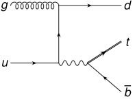
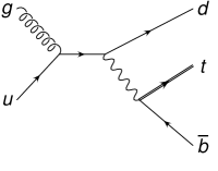
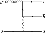
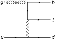
In the following, we organize and label all the Born and real subprocesses, keeping the distinction between the - and -channel contributions. This distinction holds also when real corrections are considered, since, due to color flow, interferences do not arise between real corrections to - and -channel Born processes.
-
1)
In the -channel case, there are only Born processes of the type , where and run over all possible different quark and antiquark flavours compatible with the final state. We denote with the (summed and averaged) squared amplitude, divided by the flux factor. The corresponding real correction contributions include processes with an outgoing or an incoming gluon, i.e. processes of type , and . We denote these contributions with , and . Summarizing, we have
process notation contributing subprocesses , , , , where and stand for a generic up- or down-type light quark.
-
2)
In the -channel case, there are only Born processes of the type (and ), where and run over all possible flavours and anti-flavours. Their contributions are denoted (). We use this notation since we want to keep track of the down-type quark connected to the top quark. The structure of real corrections is more complex in this case. Contributions obtained from the previous processes by simply adding an outgoing gluon, , will be denoted as . The subprocesses generated by an initial-state gluon splitting into a quark-antiquark pair are designated by for ( for ) and for ( for ). In the former case and are connected via a vertex, while the gluon splits into a pair, so the top quark is color connected with the incoming gluon. In the latter case the situation is opposite, since the gluon splits into a pair, while the incoming is directly CKM-connected to the top quark. This gives rise to a different singularities structure, which we take into account in dealing with the () and () processes separately. Summarizing
process notation contributing subprocesses , , , , , ,
where and stand for a generic up- or down-type light quark.
In order to distinguish - and -channel real processes with the
same flavour structure, we have used the subscript and on
the and contributions. As
already stated, these contributions do not interfere owing to
different color structures, so we can keep them distinct. We have
drawn a sample of Feynman diagrams for - and -channel scattering in fig. 1.
2.2 Kinematics and singularities structure
2.2.1 Born kinematics
Following the notation of ref. [24], we denote with and the incoming quark momenta, aligned along the plus and minus direction of the axis, by the outgoing top-quark momentum and by the other outgoing light-parton momentum. The final-state top-quark virtuality will be denoted by , so that . The top quark on-shell condition is , where is the top-quark mass. If and are the momenta of the incoming hadrons, then we have
| (4) |
where are the momentum fractions, and momentum conservation reads
| (5) |
We introduce the variables
| (6) |
and , the angle between the outgoing top quark and the momentum, in the partonic center-of-mass (CM) frame. We denote with the azimuthal angle of the outgoing top quark in the same reference frame. Since the differential cross sections do not depend on the overall azimuthal orientation of the outgoing partons, we set this angle to zero. At the end of the generation of an event, we perform a uniform, random azimuthal rotation of the whole event, in order to cover the whole final-state phase space. The set of variables fully parametrizes the Born kinematics. From them, we can reconstruct the momentum fractions
| (7) |
where is the squared CM energy of the hadronic collider. The outgoing momenta are first reconstructed in their longitudinal rest frame, where . In this frame, their energies are
| (8) |
The two spatial momenta are obviously opposite and both have modulus equal to . We fix the top-quark momentum to form an angle with the direction and to have zero azimuth (i.e. it lies in the plane and has positive component). Both and are then boosted back in the laboratory frame, with boost rapidity . The Born phase space, in terms of these variables, can be written as
| (9) | |||||
where
| (10) |
We generate the top quark with virtuality and decay it with a method analogous to the one adopted in ref. [37], that will be described in sec. 3.3. We take into account the top finite width by first introducing a trivial integration in eq. (9) and then by performing the replacement
| (11) |
With this substitution, the final expression for the Born phase space reads
| (12) |
2.2.2 Real-emission kinematics
Real-emission processes have an additional final-state parton that can be emitted from an incoming leg only (, , , , , ) or from both an initial- and final-state leg (, , ). We need then to use two different parametrizations of the real phase space, one to deal with initial-state singularities and one for final-state ones. We treat the radiation kinematics according to the variant of the Frixione, Kunszt and Signer (FKS) subtraction scheme [38, 39] illustrated in ref. [24]. Before giving all the technical details, we summarize briefly how the procedure works:
-
-
We split each real squared amplitude into contributions that have at most one collinear (and/or one soft) singularity.
-
-
We build the collinear (and soft) subtraction terms needed to deal with that singularity.
-
-
We choose the emission phase-space parametrization suited for the singularity we integrate on.
In the FKS method, the singular regions associated with the and legs are treated with the same kinematics. Nevertheless, we have decided to split these two different contributions in order to gain a clear subtraction structure.
We now describe the procedure used to split real squared amplitudes and the corresponding phase-space parametrizations. Subtraction terms will then be given in sec. 2.3.3. We proceed as follows:
-
1.
We start by considering real processes that have both initial- and final-state emissions, namely the , and contributions. In this case, the FKS parton is the outgoing gluon and we choose it to be the last particle. We denote its momentum by , so that momentum conservation reads
(13) where , , and label the same particles of the underlying Born process. The FKS parton can become collinear to one of the incoming legs or to the other massless final-state leg, so we need to introduce a set of functions to project out these different singular regions. The general properties these functions have to satisfy were given in sec. 2.4 of ref. [24]. In this paper we use
(14) where
(15) For any given kinematic configuration, these functions satisfy
(16) The separation among different singular regions is performed multiplying each real contribution with the corresponding function. For example, for the -channel case, we have
(17) These contributions are now singular only when the FKS parton becomes collinear to , and respectively, or soft. Analogous relations hold for and .
-
2.
Next we consider the real process . It is singular when or become collinear to the incoming gluon, so that the FKS parton can be respectively or and we need again a set of functions to project out the different singular regions. Recalling the labeling of the momenta
we introduce the projecting functions
(18) to isolate the region where or . We have then the two contributions
(19) coming from . For , analogous contributions can be obtained from eqs. (2) and (2) with the substitutions and .
-
3.
To deal with the remaining real contributions we do not need to introduce any other function, since each of them is singular in one region only (the one for and , the one for and ).
Having split all real contributions in such a way that each term has at most one singularity, we can associate with each of them a particular phase-space parametrization, suitable to handle that singularity structure. In the following we summarize the reconstruction procedure needed to build the real-emission kinematics, given the underlying Born one, and a set of three radiation variables. For all the details, we refer to sec. 5 of ref. [24].
Parametrization of the initial-state radiation (ISR) phase space
The FKS method uses the same phase-space parametrization for describing both the and singular regions. The set of radiation variables
| (20) |
together with the Born ones, completely reconstruct the real-event kinematics: . Using eq. (7), we can compute the underlying Born momentum fractions and, from them, we obtain
| (21) |
with the kinematics constraints
| (22) |
where
| (23) | |||||
In the laboratory frame, the incoming momenta are given by
| (24) |
In the partonic center-of-mass frame, we define the FKS parton to have momentum
| (25) |
where
| (26) |
and
| (27) |
From eqs. (25) and (26), we see that the soft limit is approached when , while the collinear limits are characterized by ( parallel to the direction) or ( parallel to the direction).
Boosting back in the laboratory frame with longitudinal velocity we obtain . Having computed and , we can construct , while from the underlying Born momenta we have . We construct then the longitudinal boost , with boost velocity , where
| (28) |
so that the boosted momentum has zero longitudinal component. In addition we define
| (29) |
and the corresponding (transverse) boost , so that has zero transverse momentum. The final-state momenta and in the laboratory frame are obtained with the following boost sequence
| (30) |
Finally, the three-body phase space can be written, in a factorized form, in terms of the Born and radiation phase space
| (31) |
where
| (32) |
that defines the Jacobian of the change of variables.
Parametrization of the final-state radiation (FSR) phase space
For the FSR phase-space parametrization , we use the same notation as for the initial-state case (see eq. (20)). We define, in the partonic center-of-mass frame,
| (33) |
where
| (34) |
and the notation stands for . We denote with an arbitrary direction that serves as origin for the azimuthal angle of around , while “” is the cross vector product. The notation indicates the angle between and , so that is the azimuth of the vector around the direction .***The FKS variant that we use (see ref. [24]) has a slightly different definition of than the one introduced in the original FKS papers.
From eq. (33) we see that the soft limit is approached when , while the collinear limit is characterized by ( parallel to ).
Given the set of variables we can reconstruct the full real-event kinematics. The momentum fractions are the same as the underlying Born ones, since the emission from a final-state leg does not affect them, so that
| (35) |
Inverting the first identity in eq. (33), we immediately have
| (36) |
where is limited by
| (37) |
with
| (38) |
The energy (and the modulus) of the other light outgoing parton, always in the partonic center-of-mass frame, is given by
| (39) |
Given and we construct the corresponding vectors and such that their vector sum is parallel to and the azimuth of relative to (the given reference direction) is . Having fully defined and , we can reconstruct the vector of eq. (34) and find . Finally, can be obtained boosting along the direction with boost velocity
| (40) |
or, alternatively, exploiting momentum conservation of eq. (13). To obtain the momenta in the laboratory frame we need to boost back all the outgoing momenta computed in the center-of-mass frame.
In this case too, the three-body phase space can be written in a factorized form in terms of the Born and radiation phase space
| (41) |
where
2.3 Squared amplitudes
In order to apply the POWHEG method, we need the Born, real and soft-virtual contributions to the differential cross section, i.e. the squared amplitudes, summed (averaged) over colors and helicities of the outgoing (incoming) partons, and multiplied by the appropriate flux factor. We have taken the Born, real and soft-virtual contributions from the MC@NLO code, testing, where possible, our implementation against MadGraph subroutines [40]. All the matrix elements have been evaluated in the zero-width approximation, i.e. and are set equal to zero in all the propagators. As already mentioned, to recover finite-width effects in top-decay, the top mass is generated according to a Breit-Wigner distribution, centered in and with width (see eq. (11)).
In the following, we give explicit expressions for the Born and collinear remnant contributions. Real and soft-virtual matrix elements are more complicated, and we do not report them explicitly. Nevertheless, we give the soft and collinear limits of the real amplitude, since these expressions are needed in the FKS subtraction formalism.
2.3.1 Born and virtual contributions
We denote the -channel squared matrix element for the lowest-order contribution, averaged over color and helicities of the incoming particles, and multiplied by the flux factor , as . For example, for the subprocess, we have
| (43) |
where is the usual Mandelstam variable, is the weak coupling () and ’s are the CKM matrix elements. Crossing eq. (43) we have, for the initiated process,
| (44) |
and for the -channel contributions ( and ) of the and subprocesses
| (45) |
where . The corresponding expressions for and can be obtained from the latter again by crossing. They are given by
| (46) |
The finite soft-virtual contributions, obtained according to the FKS method, have been taken from the MC@NLO code. We included them in our NLO calculation and tested the correct behaviour of our program by comparing our NLO results with the MCFM code [41], both for the full NLO cross section and for typical differential distributions. Some comparisons have also been carried out with the program ZTOP [42].
2.3.2 Collinear remnants
The collinear remnants are given in eq. (2.102)
of ref. [24]. Here we limit ourselves to list all the
contributions, giving only a couple of explicit examples to clarify the
notation.
For the -channel processes, the collinear remnants are
| (47) |
where the notation, according to ref. [24], represents the set of variables
| (48) |
The underlying Born configuration , associated with the kinematics, is defined by
| (49) |
Similar formulae hold for . Among the contributions listed in (47), only the real process is singular in both the and the region. It thus needs the two collinear remnants
| (50) | |||||
For the -channel processes, the collinear remnants are
| (51) |
In this case, contains two terms, since in the scattering both the two outgoing massless partons and can become collinear to the incoming gluon. We have
| (52) | |||||
where and are the corresponding underlying Born processes. All the other contributions can be obtained in a similar way.
2.3.3 Soft and collinear limits of the real contributions
In the FKS formalism, phase-space singular regions are approached when the radiation variables and/or . The corresponding singularities are subtracted from the real cross section using the plus distributions. One needs to express the singular limits in terms of suitable radiation variables and of the corresponding underlying Born contributions. In this section we compute these limits and give explicitly their expressions.
We start by considering the singular limits of the processes that have both ISR and FSR singularities, namely , and . These processes are the most subtle, being both soft and collinear divergent for initial- and final-state radiation. As an example, we study the limits for the -channel scattering . We can deal with ISR and FSR separately, having defined the contributions , and .
For ISR singularities, we use the set to parametrize the kinematics. When , the momentum is aligned along the direction and , in the CM frame. The real squared amplitude factorizes and we have
| (53) |
where , is the usual Altarelli-Parisi (AP) splitting kernel and we have included the real flux factor and a factor into the term, as its definition requires. In the FKS approach, one needs the finite quantity to perform the subtraction of the singularities. In the collinear limit, we have
| (54) |
In the same limit, we also note that the contributions and go to zero, because the factor makes them finite and the corresponding functions were chosen to vanish in this limit.
In the FSR case, the collinear limit is reached when . The outgoing momenta and become parallel and aligned along their sum, denoted by . Momentum conservation reads
| (55) |
and, in the partonic CM frame, one has
| (56) |
where . A factorized expression holds in this case too
| (57) |
The finite quantity needed in the application of the subtraction method is now , that is given by
| (58) |
We note again that, in this collinear limit, the contributions vanish, because of the behaviour of the functions.
The contribution is also singular when the outgoing gluon becomes soft, i.e. when . In both the two phase-space parametrizations ( and ), this limit is approached when . The Born process has more than 3 colored particles, so that, in general, one may expect that soft singularities factorize in terms of the color ordered Born amplitudes [24]. However, in this case, the color algebra simplifies, because of the exchange of an intermediate colorless particle, and we have complete factorization on the Born squared amplitude. The contribution in the soft limit (eikonal approximation) is given by
| (59) |
The radiation variable assumes different meaning in the case of ISR or FSR (see sec. 2.2.2). In the ISR case, we have the finite contributions
| (60) |
where identifies the direction of the soft gluon. In the FSR case we have instead
| (61) |
with , defined in the partonic CM frame.
The -channel processes and are dealt in an analogous way, either for the collinear and the soft limits. All the other processes have only ISR collinear singularities: the corresponding limits can be obtained from eq. (53), substituting the appropriate AP splitting kernel and the Born term.
3 The POWHEG implementation
3.1 Generation of the Born variables
In the POWHEG method, we first generate the Born kinematics according to the function, which is the integral of the full NLO cross section at a given value of the underlying Born kinematics. It is defined as follows:
| (62) |
where
| (63) |
with
and where
| (65) |
with
| (66) | |||||
The contribution can be obtained from eq. (66) by simply exchanging all flavour indexes and substituting .
According to the POWHEG notation, in eqs. (3.1) and (66) we have traded the , , and quantities with the corresponding capital letters, obtained by multiplying them with the appropriate luminosity , defined in terms of the parton distribution functions (PDF) as
| (67) |
All the integrals appearing in the above equations are now finite. In fact, following the FKS subtraction scheme, the hatted functions
| (68) |
and
| (69) |
have only integrable divergences when integrated over and respectively.†††In our case, for both the - and -channels, Some care should still be taken when dealing with the plus distributions. For more details we refer to refs. [24] and [32].
Following ref. [24], we introduce the function, defined such that its integral over the radiation variables, mapped onto a unit cube , gives
| (70) |
The generation of the Born variables is performed by using the integrator-unweighter program MINT [43] that, after a single integration of the function over the Born and radiation variables, can generate random values for the variables , distributed according to the weight . We then keep the generated values only, and neglect all the others, which corresponds to integrate over them. At this stage, we also need to choose a Born flavour structure ( in the language of ref. [24]) with a probability proportional to its relative weight in the function (see eqs. (63) and (65)). The event is then further processed, to generate the radiation variables, as illustrated in the following section.
3.2 Generation of the hardest-radiation variables
Radiation kinematics is generated using the POWHEG Sudakov form factor. For a given underlying Born kinematics () and flavour structure (), the Sudakov form factor can be expressed as
| (71) |
where one needs to include in the product all the projected real contributions that have, as singular limit, the generated underlying Born. In our case, for the -channel, we can write
| (72) |
where
| (73) | |||||
and
| (74) |
For clarity, here we indicate with the real contribution of type that corresponds to the underlying Born . The functions and measure the hardness of the radiation in the real event. In case of ISR singular processes, we chose as hardness variable the exact transverse momentum of the emitted parton with respect to the beam axis. In terms of , this is given by
| (75) |
For the FSR singular processes, instead, we use as hardness variable the exact transverse momentum of the FKS parton with respect to the other light outgoing parton, evaluated in the center-of-mass frame. In terms of , this is given by‡‡‡Since for no singularities arise in the FSR case, another possible choice for would be (76) that has the same behaviour of eq. (77) in the collinear limit but has a simpler functional form. We have checked that no sizable differences arise if one uses eq. (76) instead of eq. (77).
| (77) |
The generation of the hardest radiation is performed individually for and , and the highest generated is retained. This corresponds to generate according to eq. (72), as shown in Appendix B of ref. [24]. If is below a given cut, , no radiation is generated, and a Born event is returned.
The upper bounding functions for the application of the veto method have been chosen in the following way:
| (78) |
for ISR, and
| (79) |
for FSR.
The same procedures holds also for the -channel case, with appropriate modifications in formulae (72)–(79).
The method used to generate radiation events according to these upper bounding functions is analogous to the one described in Appendix D of ref. [25], and we do not repeat it here.
As a final remark, we also point out that single-top - and -channel Born cross sections vanish at some points in the Born phase space, as one can argue by looking at eqs. (43)–(2.3.1). For this reason, special care has to be taken during the radiation generation procedure. We handled this problem using the same method described in sec. 3.3 of ref. [29]. We thus refer to that paper for further details.
3.3 Top-quark decay
The calculation we have described so far leads to the generation of events with an undecayed top quark. We include the decay kinematics effects in an approximate way, by requiring that the decay products are distributed with a probability proportional to the tree-level cross section for the full production and decay process. This procedure was first suggested in ref. [37]. In the following we describe our implementation, focusing upon the decay .
We first generate a Born-like or real-like event according to the POWHEG method. In both cases we denote the set of variables that parametrize the undecayed momenta as and the corresponding flavour structure as . As described at the end of sec. 2.2.1, at this stage the top virtuality is distributed according to a Breit-Wigner function. We write the tree-level cross section for production and decay in the following form
| (80) |
where is the luminosity factor and is the squared amplitude corresponding to the full decayed process that originates from the undecayed process .§§§The full tree-level squared amplitudes have been obtained using MadGraph. For consistency, the squared amplitude must include only resonant graphs (i.e. graphs where the top momentum equals the sum of the , and momenta). We write the full phase space, including the decay, in the factorized form
| (81) |
where is the undecayed (POWHEG) phase space and is defined implicitly by this equation. We notice that
| (82) |
where is the undecayed squared amplitude, i.e. the Born or real amplitude that we used throughout the computation. Thus, the differential probability for the generation of from a given undecayed kinematics is
| (83) |
To generate efficiently distributed according to (83) we use the hit-and-miss technique and so we need to find an upper bounding function for . This bound can be guessed from the structure of the top decay. In our case, we use as upper bound for the ratio , the expression
| (84) |
where and and are the decay squared amplitudes corresponding to the subprocesses in their subscripts. In the previous formula, as well as in , finite-width effects have been fully taken into account. One can predict the appropriate value for the normalization factor as explained in ref. [37] or compute it by sampling the decay phase space and comparing with the exact expression, in such a way that the inequality
| (85) |
holds. The veto algorithm is then applied:
-
1.
First one generates a point in the phase space .
-
2.
Then a random number in the range is generated.
-
3.
If , keep the decay kinematics and generate the event. Otherwise go back to step 1.
4 Results
In this section we present our results and comparisons with the fixed order (next-to-leading) calculation and with the MC@NLO 3.3 and PYTHIA 6.4.21 Shower Monte Carlo (SMC) programs.¶¶¶This newest update of PYTHIA yields more consistent results when multiple interactions are turned on in user-initiated processes (see the release notes in http://projects.hepforge.org/pythia6/). We have used the CTEQ6M [44] set for the parton distribution functions and the associated value of GeV. Furthermore, as discussed in refs. [24, 25], we use a rescaled value in the expression for appearing in the Sudakov form factors, in order to achieve next-to-leading logarithmic accuracy.
Although the matrix-element calculation has been performed in the massless-quark limit (except, of course, for the top quark), the lower cutoff in the generation of the radiation has been fixed according to the mass of the emitting quark. The lower bound on the transverse momentum for the emission off a massless emitter (, , ) has been set to the value . We instead choose equal to or when the gluon is emitted by a charm or a bottom quark, respectively. We set GeV and GeV.
The renormalization and factorization scales have been taken equal to the radiated transverse momentum during the generation of radiation (see eqs. (75) and (77)), as the POWHEG method requires. We have also taken into account properly the heavy-flavour thresholds in the running of and in the PDF’s, by changing the number of active flavours when the renormalization or factorization scales cross a mass threshold. In the calculation, instead, and have been chosen equal to the top-quark mass, whose value has been fixed to GeV. In all the comparisons, we have kept the top-quark virtuality fixed to , so that matrix elements have been evaluated assuming . We have also set in all the propagators. The other relevant parameters are
| (86) |
From the above values, the weak coupling has been computed as . In addition, for sake of comparison, we fixed the CKM matrix elements equal to
| (87) |
In order to minimize effects due to differences in the shower and hadronization algorithms, we have interfaced POWHEG with the HERWIG angular-ordered shower when comparing with MC@NLO and with the -ordered PYTHIA shower when comparisons with PYTHIA have been carried out.
All the following results have been obtained assuming that the top decays semileptonically (), as explained in sec. 3.3, but removing the branching ratio, so that plots are normalized to the total cross section.
We present a few distributions, done mainly for comparison with MC@NLO and with the NLO calculation. Some of them are “unphysical”, i.e., for example, when talking of the top-quark momentum , we refer to the exact taken directly from the MC shower history, right before the top decay. For sake of simplicity, we also force the lightest -flavoured hadrons to be stable after the hadronization stage of SMC programs.
Jets have been defined according to the algorithm [45], as implemented in the FASTJET package [46], setting and imposing a lower GeV cut on jet transverse momenta. We call “top jet” the jet that contains the hardest -flavoured hadron,∥∥∥Here we mean precisely -flavoured, i.e. not -flavoured, that arises in the production process. which will, most of the time, come from the top-quark decay. The other reconstructed jets will come from the shower of massless partons, and we call them “light jets”.******In the fixed-order calculation, instead, the top quark is not decayed, and the top jet corresponds to the jet that contains the top quark. In this way, the momentum of the top quark and the momentum of the top jet are different, since the last may or may not include all the particles from the top decay and shower.
4.1 Tevatron results
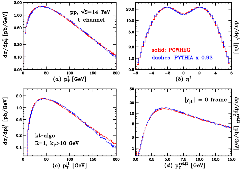
We start comparing various kinematical variables for single-top -channel production at the Tevatron collider. In fig. 2 we have collected the following distributions:
-
•
In panels (a) and (b) we show the transverse momentum and the pseudorapidity of the top quark and in panel (c) we show the hardest jet transverse momentum . The agreement with the fixed-order calculation and with the MC@NLO results is very good. Only the top transverse-momentum distribution shows a tiny mismatch, our result being slightly softer than the NLO and the MC@NLO ones. When interfacing POWHEG with PYTHIA, we instead find full overlapping with the NLO result. It is thus likely that this small feature may be attributed to shower effects.
-
•
In panel (d), we plot , the relative transverse momentum of all the particles clustered inside the hardest jet. This is defined as follows:
-
–
We perform a longitudinal boost to a frame where the hardest-jet rapidity is zero.
-
–
In this frame, we compute the quantity
(88) where ’s are the momenta of the particles that belong to the hardest jet that, in this frame, has momentum .
This quantity is thus the sum of the absolute values of the transverse momenta, taken with respect to the jet axis, of the particles inside the hardest jet, in the frame specified above. The plot shows a marked disagreement between fixed order calculation and showered results. This disagreement is well understood, since the observable we are considering is a measure of the spreading of the hardest jet. Thus, its shape is strongly affected by the Sudakov form factor and it is well described by SMC programs. The NLO calculation cannot give, instead, a reliable estimate, since when the differential cross section diverges.
-
–
-
•
In plots (e) and (f), the next-to-hardest jet transverse momentum , and the transverse momentum of the system made by the top quark and the hardest jet, , are shown. We see a remarkable good agreement between our program and MC@NLO, while sensible differences with respect to the NLO results are present. At the NLO parton level, and balance against each other, so that the two distributions coincide down to the minimum cut present in the first plot.
In plot (e), we see an enhancement of the showered results at intermediate values of , while in plot (f) we see a low- suppression and an enhancement at intermediate and high . The low- suppression is clearly a Sudakov effect. The high- enhancement comes instead from events in which the hardest parton is well balanced against the top quark, but where many hadrons, coming from the hardest parton, end up in the top jet, and are thus removed, or they end up out of the jet cluster. This creates an artificial imbalance, and thus an effective for the system. These effects are so pronounced because the cross section for a balanced top-quark–hardest-jet system is much higher, since it does not require the production of an additional hard parton. We have verified this hypothesis by analyzing POWHEG outputs before the showering stage, either clustering or not the quark coming from the top decay. In the case where the quark is included in the analysis (and the jet containing the is removed from the jet sample), we see a marked rise of the tail. A further rise is observed when the shower is turned on, and may be attributed to energy lost out of the hardest jet cluster due to showering. We see no such effect for the next-to-hardest jet spectrum in plot (e). There, the raise at medium may be attributed to the shower smearing.
-
•
Finally, in plots (g) and (h), the pseudorapidity of the top-quark–hardest-jet system and the azimuthal difference are shown. The pseudorapidity of the system shows an expected discrepancy between the showered results and the fixed order one: radiation near the beam axis is suppressed by the Sudakov form factor but not in the NLO result, giving rise to the higher tails at large . In plot (h), MC@NLO and POWHEG differ instead from the fixed order result for a kinematical reason: at the parton level, having at most three particles, there is no phase space for the next-to-hardest jet to recoil against the system when .


A similar set of comparisons is presented in fig. 3 for the -channel production mechanism, always at the Tevatron. The agreement between POWHEG and MC@NLO is as good as before for inclusive quantities, or even better. In particular, the slight mismatch in the top transverse-momentum distribution completely disappears, as one can see in plot (a). For all the other plots, considerations similar to the -channel case remain valid.
In fig. 4 the same set of plots are shown, comparing POWHEG and PYTHIA. We have good agreement for most distributions, after applying an appropriate factor to the PYTHIA results. Only minor differences are present in the high- tail of distributions in panels (e) and (f).
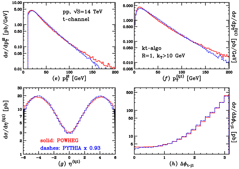
As a final comparison, in the left panel of fig. 5, we show , the transverse-momentum spectrum of the hardest -flavoured hadron, after imposing the rapidity cut . In the -channel, this hadron will come most probably from an initial-state gluon undergoing a splitting. The quark is then turned into a while the quark is showered and hadronized. We see that, while POWHEG and MC@NLO are in a fair agreement in the medium- and high- range, sizable differences are present at low . These discrepancies are most probably due to the disagreement that one can notice in the distribution (right panel of fig. 5), and to a smaller extent to a different implementation of the inclusion of -mass effects by both programs (just before the showering stage).

We also plot in fig. 6 the same quantities comparing POWHEG interfaced to PYTHIA with respect to PYTHIA alone. A large mismatch in the high- spectrum is clearly visible in the left panel. This observable is particularly sensitive to real matrix-element effects, not present in PYTHIA. Concerning the low- behaviour, we see that here the difference is much less pronounced than in fig. 5. Furthermore, the aforementioned mismatch in the distribution is no longer present, as one can see in the right panel.

By comparing figs. 5 and 6, one immediately notices the different behaviours of the two Monte Carlo programs that we are interfacing to. We observe that the HERWIG shower and hadronization create an enhancement at large values of , which is not present in PYTHIA. This feature is known to the HERWIG authors,††††††See M. Seymour’s talk in http://bwhcphysics.lbl.gov/vplusjets.html. and is traced back to a mismatch of the scale at which backward evolution is switched off, with the scale at which the -quark density is turned on in the pdf’s. The effect is more pronounced in MC@NLO, probably due to the fact that POWHEG does not rely on HERWIG for the generation of the hardest splitting.
4.2 LHC results
In figs. 7 and 8 similar results are reported for the LHC collider. Only plots for the -channel production are shown, the -channel process having a negligible impact at the LHC.
Figure 7 contains comparisons between POWHEG, MC@NLO and NLO results. No significant differences with respect to what we observed at the Tevatron arise in any plot, so that we refer to the previous section for comments.
In the PYTHIA and POWHEG comparisons shown in fig. 8, we immediately notice that the POWHEG enhancement of high- tails in panels (e) and (f) is here more marked, even if still small. This may again be related to the lack of matrix-element corrections in PYTHIA, resulting in larger discrepancies at the LHC with respect to the Tevatron case.
In panels (c) and (e), one can also notice different low- shapes with respect to the same plots showing the POWHEG+HERWIG results of fig. 7. We have verified that these differences are due to the inclusion of multiple interactions (MI) in the default PYTHIA.‡‡‡‡‡‡These account for events where more than one parton pair in the same incoming hadrons give rise to hard interactions. If we limit ourselves to the results without MI (i.e. setting MSTP(81)=0 in PYTHIA), the agreement is much better.

4.3 Top-quark decay
As explained in sec. 3.3, in our calculation we have implemented spin correlations in top decay. Sizable effects are thus visible when comparing our results with SMC programs that do not implement them. MC@NLO accounts for these effects with approximately the same method that we use. Hence, we expect to have good agreement with MC@NLO and visible discrepancies when comparing with PYTHIA.
Due to the V-A structure of the weak current, the best observables to highlight eventual discrepancies are those involving the angle between the charged lepton coming from top decay and the direction of the down-type quark entering the vertex involved in top production, as shown in fig. 9.


At the Born level, the down-type quark direction is possibly identified with the beam axis for -channel production, while, for -channel production, it often corresponds to the hardest jet axis (see ref. [47] for further details).
For sake of comparison, we have set the top virtuality and we have taken the values GeV and GeV in the evaluation of upper bounds of the decay amplitudes in eq. (84) and in the decayed matrix element . Furthermore, we have applied cuts similar to those used in ref. [37], both for the Tevatron and for the LHC, namely
| (89) | |||
| (90) | |||
| (91) |
We denote with the superscript the top jet, i.e. the jet that contains the hardest -flavoured hadron (not the ). In single-top processes, this comes almost exclusively from the bottom quark emerging from top decay. In -channel production, in order to isolate a central hardest light jet, we apply the further cuts
| (92) |
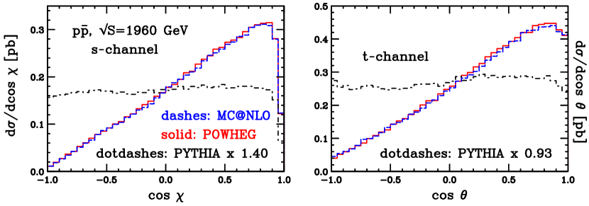
In fig. 10 we show comparisons for the Tevatron collider. On the left panel, we plot the -channel differential cross section as a function of , where is the angle between the hardest charged lepton , which we assume coming from top decay, and the direction of the incoming parton with negative rapidity (the direction of the axis), as seen in the top rest frame. Such angle is sensitive to the spin correlation between and the incoming quark, which, at the Tevatron, is pulled out mostly from the antiproton traveling in the negative direction. On the right panel, we plot the -channel differential cross section as a function of , where is the angle between and the hardest jet, always evaluated in the top rest frame. In both plots, we observe a remarkable good agreement with MC@NLO and the expected discrepancy with PYTHIA, that only performs a spin-averaged top decay.

In fig. 11 we plot the transverse momentum and pseudorapidity of the hardest charged lepton, for -channel production at Tevatron. The difference between PYTHIA and POWHEG (or MC@NLO) can be shown to arise because of spin-correlation effects. To test this, we run POWHEG with an undecayed top in the final state, leaving PYTHIA to perform the decay: after rescaling the plots with the appropriate factor, we obtain the same behaviour as PYTHIA standalone.
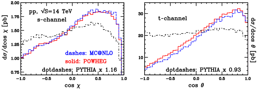
In fig. 12, the same distributions of fig. 10 are shown for the LHC collider. The same considerations done for the Tevatron apply for the LHC results.
4.4 Dips in the rapidity distributions
In previous works [25, 26, 29, 32], we have extensively discussed the presence of sizable mismatches between POWHEG and MC@NLO results in the rapidity difference between the hardest jet and the heavy system recoiling against it. More specifically, the MC@NLO results exhibit, for this quantity, a dip at zero rapidity, not visible in POWHEG. This problem was originally pointed out in ref. [48] in the framework of production, and its origin was traced back to HERWIG, that shows an even deeper dip for the same quantity. In ref. [33], in the framework of Higgs production, this problem and its Shower Monte Carlo origin was accurately studied.
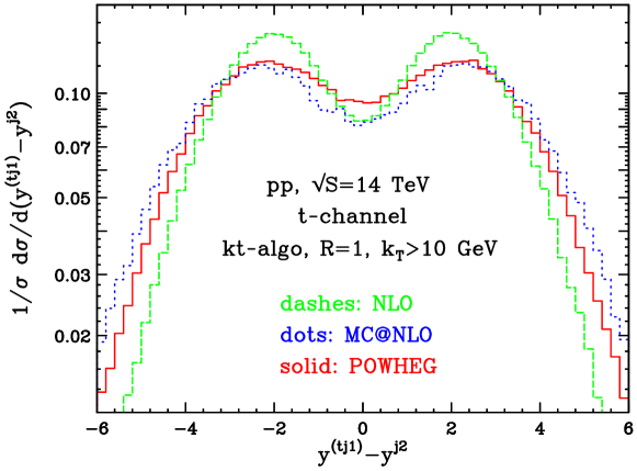
In single-top production, the suitable quantity where to observe this mismatch is the rapidity difference between the top-quark–hardest-jet system and the next-to-hardest jet. As one can see in fig. 13, in this case a dip in the central rapidity region is already present at the next-to-leading order. This feature may mask an eventual dip in MC@NLO. In fact, the two showered results are fairly similar, with the dip being slightly more pronounced in MC@NLO.
In recent talks [49, 50, 51], one of us proposed a possible explanation of the presence of these dips in the MC@NLO results. In the following we illustrate this explanation and show that it is also compatible with the case at hand.
We can schematically represent the MC@NLO cross section for the hardest emission with the following formula
| (93) | |||||
The terminology “” and “ events” is defined in the original MC@NLO papers [19, 20]. We have
| (94) | |||||
| (95) | |||||
| (96) |
where are the Altarelli-Parisi splitting kernels and . Notice that, on the right hand side of eq. (94), divergent quantities appear, and only their sum is finite. In the MC@NLO framework, they are dealt with the subtraction method.
The “MC shower” factor in eq. (93) shows that the hardest emission is produced by running the HERWIG shower Monte Carlo, starting with the event kinematics . In fact, the Monte Carlo may not generate the hardest radiation as its first emission. It was shown in ref. [23], however, that formula (93) does correctly represent the hardest emission probability up to subleading effects, that we here assume to be irrelevant for our argument.
In the production of a high- parton, formula (93) yields
| (97) | |||||
where we have used the fact that in this limit. The first term correctly describes the hard radiation in the whole phase space. The second term, while formally subleading in , is responsible for the dip. In fact, the dip present in HERWIG propagates here with a weight proportional to . Although subleading, this term can be significant for processes with large factors.
In the processes studied so far, this ratio was significantly higher than 1 (see, for example, ), so that the effect was particularly visible. In single-top production, instead, due to the small NLO factor, one has . This, together with the fact that the fixed NLO result already presents a central dip for , results in small discrepancies between MC@NLO and POWHEG (see fig. 13).
We notice that a similar mechanism (i.e. via a large factor) for generating large NNLO terms operates also in POWHEG, and has been discussed in ref. [32] in the framework of Higgs production, as being responsible for a hard Higgs boson spectrum. In POWHEG, however, this mechanism cannot generate any dip, since here HERWIG has no role in the generation of the hardest radiation.
5 Conclusions
In this paper we have described a complete implementation of - and -channel single-top production at next-to-leading order in QCD, in the POWHEG framework. This is the first POWHEG implementation of a process where both initial- and final-state radiation is present. The calculation for top production has been performed within the Frixione-Kunszt-Signer subtraction approach [38, 39], modified according to ref. [24]. We accounted for spin-correlation effects in top-quark decay with a method analogous to the one proposed in ref. [37]. The results of our work have been extensively compared with the MC@NLO and PYTHIA Shower Monte Carlo programs, together with the fixed next-to-leading order calculation, both for the Tevatron and for the LHC.
The MC@NLO results are in good agreement with POWHEG, also for quantities sensitive to angular correlations in top decay.
The PYTHIA results, normalized to the total NLO cross section, show fair agreement with ours for inclusive quantities that do not involve the top-decay products. As expected, we have found sizable mismatches with PYTHIA when considering distributions involving top-decay products, such as angular-correlation measurements and charged-lepton transverse momentum and pseudorapidity. We have also found differences between our results and the MC@NLO and PYTHIA ones in the hardest -flavoured hadron transverse momentum and rapidity. The high- mismatch with PYTHIA may be a consequence of the lack of matrix-element corrections in the latter, while we attribute the low- disagreement with MC@NLO to the sizable difference that we observe in the rapidity distribution.
The computer code for the POWHEG implementation presented in this paper is available, together with the manual, at the site http://moby.mib.infn.it/~nason/POWHEG.
Acknowledgments
We thank Mike Seymour and Torbjörn Sjöstrand for useful discussions.
References
- [1] CDF Collaboration, T. Aaltonen et al., First Observation of Electroweak Single Top Quark Production, arXiv:0903.0885.
- [2] D0 Collaboration, V. M. Abazov et al., Observation of Single Top Quark Production, arXiv:0903.0850.
- [3] M. Beneke et al., Top quark physics, hep-ph/0003033.
- [4] B. W. Harris, E. Laenen, L. Phaf, Z. Sullivan, and S. Weinzierl, The Fully differential single top quark cross-section in next to leading order QCD, Phys. Rev. D66 (2002) 054024, [hep-ph/0207055].
- [5] J. Alwall et al., Is ?, Eur. Phys. J. C49 (2007) 791–801, [hep-ph/0607115].
- [6] G. Mahlon and S. J. Parke, Improved spin basis for angular correlation studies in single top quark production at the Tevatron, Phys. Rev. D55 (1997) 7249–7254, [hep-ph/9611367].
- [7] G. Mahlon and S. J. Parke, Single top quark production at the LHC: Understanding spin, Phys. Lett. B476 (2000) 323–330, [hep-ph/9912458].
- [8] T. M. P. Tait and C. P. Yuan, Single top quark production as a window to physics beyond the standard model, Phys. Rev. D63 (2001) 014018, [hep-ph/0007298].
- [9] Q.-H. Cao, J. Wudka, and C. P. Yuan, Search for New Physics via Single Top Production at the LHC, Phys. Lett. B658 (2007) 50–56, [arXiv:0704.2809].
- [10] T. Plehn, M. Rauch, and M. Spannowsky, Understanding Single Tops using Jets, arXiv:0906.1803.
- [11] G. Bordes and B. van Eijk, Calculating QCD corrections to single top production in hadronic interactions, Nucl. Phys. B435 (1995) 23–58.
- [12] T. Stelzer, Z. Sullivan, and S. Willenbrock, Single top quark production via -gluon fusion at next-to-leading order, Phys. Rev. D56 (1997) 5919–5927, [hep-ph/9705398].
- [13] Z. Sullivan, Understanding single-top-quark production and jets at hadron colliders, Phys. Rev. D70 (2004) 114012, [hep-ph/0408049].
- [14] J. M. Campbell, R. K. Ellis, and F. Tramontano, Single top production and decay at next-to-leading order, Phys. Rev. D70 (2004) 094012, [hep-ph/0408158].
- [15] J. M. Campbell and F. Tramontano, Next-to-leading order corrections to production and decay, Nucl. Phys. B726 (2005) 109–130, [hep-ph/0506289].
- [16] Q.-H. Cao, R. Schwienhorst, and C. P. Yuan, Next-to-leading order corrections to single top quark production and decay at Tevatron. 1. -channel process, Phys. Rev. D71 (2005) 054023, [hep-ph/0409040].
- [17] Q.-H. Cao, R. Schwienhorst, J. A. Benitez, R. Brock, and C. P. Yuan, Next-to-leading order corrections to single top quark production and decay at the Tevatron: 2. -channel process, Phys. Rev. D72 (2005) 094027, [hep-ph/0504230].
- [18] J. M. Campbell, R. Frederix, F. Maltoni, and F. Tramontano, -channel single-top production at hadron colliders, arXiv:0903.0005.
- [19] S. Frixione and B. R. Webber, Matching NLO QCD computations and parton shower simulations, JHEP 06 (2002) 029, [hep-ph/0204244].
- [20] S. Frixione, P. Nason, and B. R. Webber, Matching NLO QCD and parton showers in heavy flavour production, JHEP 08 (2003) 007, [hep-ph/0305252].
- [21] S. Frixione, E. Laenen, P. Motylinski, and B. R. Webber, Single-top production in MC@NLO, JHEP 03 (2006) 092, [hep-ph/0512250].
- [22] S. Frixione, E. Laenen, P. Motylinski, B. R. Webber, and C. D. White, Single-top hadroproduction in association with a W boson, JHEP 07 (2008) 029, [arXiv:0805.3067].
- [23] P. Nason, A new method for combining NLO QCD with shower Monte Carlo algorithms, JHEP 11 (2004) 040, [hep-ph/0409146].
- [24] S. Frixione, P. Nason, and C. Oleari, Matching NLO QCD computations with Parton Shower simulations: the POWHEG method, JHEP 11 (2007) 070, [arXiv:0709.2092].
- [25] P. Nason and G. Ridolfi, A positive-weight next-to-leading-order Monte Carlo for pair hadroproduction, JHEP 08 (2006) 077, [hep-ph/0606275].
- [26] S. Frixione, P. Nason, and G. Ridolfi, A Positive-Weight Next-to-Leading-Order Monte Carlo for Heavy Flavour Hadroproduction, JHEP 09 (2007) 126, [arXiv:0707.3088].
- [27] O. Latunde-Dada, S. Gieseke, and B. Webber, A positive-weight next-to-leading-order Monte Carlo for annihilation to hadrons, JHEP 02 (2007) 051, [hep-ph/0612281].
- [28] O. Latunde-Dada, Applying the POWHEG method to top pair production and decays at the ILC, Eur. Phys. J. C58 (2008) 543–554, [arXiv:0806.4560].
- [29] S. Alioli, P. Nason, C. Oleari, and E. Re, NLO vector-boson production matched with shower in POWHEG, JHEP 07 (2008) 060, [arXiv:0805.4802].
- [30] K. Hamilton, P. Richardson, and J. Tully, A Positive-Weight Next-to-Leading Order Monte Carlo Simulation of Drell-Yan Vector Boson Production, JHEP 10 (2008) 015, [arXiv:0806.0290].
- [31] A. Papaefstathiou and O. Latunde-Dada, NLO production of bosons at hadron colliders using the MC@NLO and POWHEG methods, arXiv:0901.3685.
- [32] S. Alioli, P. Nason, C. Oleari, and E. Re, NLO Higgs boson production via gluon fusion matched with shower in POWHEG, JHEP 04 (2009) 002, [arXiv:0812.0578].
- [33] K. Hamilton, P. Richardson, and J. Tully, A Positive-Weight Next-to-Leading Order Monte Carlo Simulation for Higgs Boson Production, JHEP 04 (2009) 116, [arXiv:0903.4345].
- [34] G. Corcella et al., HERWIG 6: An event generator for hadron emission reactions with interfering gluons (including supersymmetric processes), JHEP 01 (2001) 010, [hep-ph/0011363].
- [35] G. Corcella et al., Herwig 6.5 release note, hep-ph/0210213.
- [36] T. Sjostrand, S. Mrenna, and P. Skands, Pythia 6.4 physics and manual, JHEP 05 (2006) 026, [hep-ph/0603175].
- [37] S. Frixione, E. Laenen, P. Motylinski, and B. R. Webber, Angular correlations of lepton pairs from vector boson and top quark decays in Monte Carlo simulations, JHEP 04 (2007) 081, [hep-ph/0702198].
- [38] S. Frixione, Z. Kunszt, and A. Signer, Three-jet cross sections to next-to-leading order, Nucl. Phys. B467 (1996) 399–442, [hep-ph/9512328].
- [39] S. Frixione, A general approach to jet cross sections in QCD, Nucl. Phys. B507 (1997) 295–314, [hep-ph/9706545].
- [40] J. Alwall et al., MadGraph/MadEvent v4: The New Web Generation, JHEP 09 (2007) 028, [arXiv:0706.2334].
- [41] http://mcfm.fnal.gov.
- [42] http://home.fnal.gov/zack/ZTOP/ZTOP.html.
- [43] P. Nason, MINT: a Computer Program for Adaptive Monte Carlo Integration and Generation of Unweighted Distributions, arXiv:0709.2085.
- [44] J. Pumplin et al., New generation of parton distributions with uncertainties from global QCD analysis, JHEP 07 (2002) 012, [hep-ph/0201195].
- [45] S. Catani, Y. L. Dokshitzer, M. H. Seymour, and B. R. Webber, Longitudinally invariant clustering algorithms for hadron-hadron collisions, Nucl. Phys. B406 (1993) 187–224.
- [46] M. Cacciari and G. P. Salam, Dispelling the myth for the jet-finder, Phys. Lett. B641 (2006) 57–61, [hep-ph/0512210].
- [47] Z. Sullivan, Angular correlations in single-top-quark and Wjj production at next-to-leading order, Phys. Rev. D72 (2005) 094034, [hep-ph/0510224].
- [48] M. L. Mangano, M. Moretti, F. Piccinini, and M. Treccani, Matching matrix elements and shower evolution for top-quark production in hadronic collisions, JHEP 01 (2007) 013, [hep-ph/0611129].
-
[49]
P. Nason, Shower Monte Carlo at Next-to-Leading Order,
http://theory.fi.infn.it/research/nason.pdf.
Talk given at the Università degli Studi di Firenze, Florence, Italy, 2009. -
[50]
P. Nason, MC at NLO tools,
http://indico.cern.ch/getFile.py/access?contribId=2&resId=0&materialId=
slides&confId=49675.
Talk given at MC4LHC Meeting, CERN, Switzerland, 2009. -
[51]
P. Nason, POWHEG,
http://agenda.hep.wisc.edu/materialDisplay.py?contribId=13&materialId=
slides&confId=189.
Talk given at LoopFest Symposium, Madison, WI, USA, 2009.