Complete versus incomplete definitions of the deformed logarithmic and exponential functions

Abstract

The recent generalizations of Boltzmann-Gibbs statistics mathematically relies on the deformed logarithmic and exponential functions defined through some deformation parameters. In the present work, we investigate whether a deformed logarithmic/exponential map is a bijection from $\mathbb{R}^{+}/\mathbb{R}$ (set of positive real numbers/all real numbers) to $\mathbb{R}/\mathbb{R}^{+}$, as their undeformed counterparts. We show that their inverse map exists only in some subsets of the aforementioned (co)domains. Furthermore, we present conditions which a generalized deformed function has to satisfy, so that the most important properties of the ordinary functions are preserved. The fulfillment of these conditions permits us to determine the validity interval of the deformation parameters. We finally apply our analysis to Tsallis, Kaniadakis, Abe and Borges-Roditi deformed functions.

LABEL:FirstPage1 LABEL:LastPage#11

I Introduction

In order to generalize the Boltzmann–Gibbs (BG) entropy and associated statistics, there have been a multitude of entropy definitions such as Tsallis Tsallis1988 , Kaniadakis Kaniadakis02 , Borges-Roditi (BR) BorgesRoditi , Abe Abe97 and Rényi Renyi1970 generalized entropies. Central goal of these generalizations is the derivation of non-exponential distributions, observed in a large number of phenomena in various fields of physical sciences involving, among others, long-range correlations, non-ergodicity, long-time memories, (multi)fractal structures and self-similarities. An important thermostatistics in this regard is the one proposed originally by Tsallis ($q$-statistics) Tsallis1988 , yielding asymptotically inverse power law distributions. The $q$-statistics has been applied to a vast number of physical situations in various scientific areas, of which a comprehensive review can be found in Ref. Tsnewbook . Similarly, one can obtain power law distributions in the thermodynamic limit through a different generalization introduced by Kaniadakis ($\kappa$-statistics) Kaniadakis02 ; KaniadQuaratiScarf ; Kaniadakis05 , developed in the context of special relativity.

Considering trace-form entropies, $\sum_{i}\Lambda_{\boldsymbol{\xi}}(p_{i})=$ $\sum_{i}p_{i}\frac{\Lambda_{\boldsymbol{\xi}}(p_{i})}{p_{i}}$, where $\boldsymbol{\xi}=\{\xi_{j}\}_{j=1,\ldots,u}$ is a deformation parameter set, $p_{i}$ is the probability of the $i$th-microstate and $\Lambda_{\boldsymbol{\xi}}(p_{i})$ is a probability functional, the generalization procedure consists of introducing deformed logarithmic and exponential functions Oik-Tirn2008 , $f_{\boldsymbol{\xi}}:\mathbb{F}^{+}\subseteq\mathbb{R}^{+}\rightarrow\mathbb{F}\subseteq\mathbb{R}$ with $f_{\boldsymbol{\xi}}(x):=x\,\Lambda_{\boldsymbol{\xi}}(1/x)$ where $\mathbb{F}\,(\mathbb{F}^{+})$ is a subset of all (positive) real numbers. Similarly, the deformed inverse function $f^{-1}_{\boldsymbol{\xi}}$ is a mapping, namely, $f^{-1}_{\boldsymbol{\xi}}:\mathbb{F}\subseteq\mathbb{R}\rightarrow\mathbb{F}^{+}\subseteq\mathbb{R}^{+}$ with $f^{-1}_{\boldsymbol{\xi}}(x):=\mathrm{Inverse}\{x\,\Lambda_{\boldsymbol{\xi}}(1/x)\}$. These deformed functions are required to recover the ordinary definitions for specific (and unique) values $\boldsymbol{\xi}_{0}$ of the deformation parameters i.e., $f_{\boldsymbol{\xi}_{0}}(x)=\ln(x)$ and $f^{-1}_{\boldsymbol{\xi}_{0}}(x)=\exp(x)$. The aforementioned $\boldsymbol{\xi}$–generalized functions usually present mathematical properties which differ from the ordinary, undeformed ones. For example, we generally observe for the deformed logarithms

$$f_{\boldsymbol{\xi}}(x\,y) \neq f_{\boldsymbol{\xi}}(x)+f_{\boldsymbol{\xi}}(y)$$ (1)

when $\boldsymbol{\xi}\neq\boldsymbol{\xi}_{0}$. Equivalently, assuming the existence of the inverse function $f^{-1}_{\boldsymbol{\xi}}(x)$, the equation above can be written in terms of the deformed exponentials as

$$f^{-1}_{\boldsymbol{\xi}}(x+y) \neq f^{-1}_{\boldsymbol{\xi}}(x)\,f^{-1}_{\boldsymbol{\xi}}(y).$$ (2)

These two equations exhibit the underlying mathematical structure of the generalized exponentials and their inverses, namely, the generalized logarithms. Evidently, the introduction of the deformation parameter $\boldsymbol{\xi}$ serves as a coupling between the variables $x$ and $y$.

In this paper, we first show that deformed functions are generally not invertible in the entire (co)domains of the ordinary functions as a consequence of the aforementioned inequalities. In this sense, the deformed functions used so far are found to be incomplete. Then, we present the conditions under which bijectivity is satisfied. Incorporating these conditions, we define complete generalized logarithms and exponentials. Finally, we apply the criterion of completeness to Tsallis, Kaniadakis, Abe and Borges-Roditi generalized functions in order to elucidate some obscure points in diverse mathematical constructions within the frame of generalized BG-Statistics. As a result of our study, it becomes evident, that the justification of whether a function can be considered as generalized logarithmic or generalized exponential function is associated with some additional properties than just a recovering limit $\boldsymbol{\xi}\rightarrow\boldsymbol{\xi}_{0}$.

The paper is organized as follows. In Section II we present the origin of the non-bijectivity of the $\boldsymbol{\xi}$-logarithm (-exponential) from $\mathbb{R}^{+}$ ($\mathbb{R}$) to $\mathbb{R}$ ($\mathbb{R}^{+}$). In order to assure the invertibility of the $\boldsymbol{\xi}$-functions in the aforementioned sets, we introduce a dependence between deformation parameters and specific subsets $\mathbb{L}_{i}$ and $\mathbb{K}_{i}$ of $\mathbb{R}^{+}$ ($\mathbb{R}^{+}=\bigcup_{i=1}^{n=2}\mathbb{L}_{i}$) and $\mathbb{R}$ ($\mathbb{R}=\bigcup_{i=1}^{n=2}\mathbb{K}_{i}$), respectively. Through the requirement of bijectivity, we are able to determine explicitly the subsets $\mathbb{L}_{i}$ and $\mathbb{K}_{i}$. In addition, we set forth conditions which permit us the determination of the respective parameter validity ranges. In Section III, we apply our formalism to Tsallis, Kaniadakis, Abe and Borges-Roditi generalized functions in order to obtain concomitant complete expressions. Finally, the main results will be summarized in Section IV.

II Definition intervals of deformed functions

We first define the following intervals $\mathbb{L}_{0}:=\{x\in\mathbb{R}:0<x\leqslant 1\}$, $\mathbb{L}_{1}:=\{x\in\mathbb{R}:x\geqslant 1\}$ so that $\mathbb{L}_{0}\bigcup\mathbb{L}_{1}=$ $\mathbb{R}^{+}:=\{x\in\mathbb{R}:x>0\}$ i.e., the set of all positive real numbers. We also choose the intervals $\mathbb{K}_{1}$ and $\mathbb{K}_{2}$ as $\mathbb{R}^{+}_{0}:=\{x\in\mathbb{R}:x\geqslant 0\}$ and $\mathbb{R}_{0}^{-}:=\{x\in\mathbb{R}:x\leqslant 0\}$, respectively so that $\mathbb{R}=\mathbb{R}^{-}_{0}\bigcup\mathbb{R}^{+}_{0}$ is the set of all real numbers. We denote the parameter validity ranges of the respective parameters $\boldsymbol{\xi}$ by $\mathcal{A}_{\boldsymbol{\xi}}\subseteq\mathbb{R}$. A boundary value of $\mathcal{A}_{\boldsymbol{\xi}}$ is always $\boldsymbol{\xi}_{0}$ e.g., $\mathcal{A}_{\boldsymbol{\xi}}:=(\alpha,\boldsymbol{\xi}_{0}]$ with $\alpha<\boldsymbol{\xi}_{0}$ or $\mathcal{A}_{\boldsymbol{\xi}}:=[\boldsymbol{\xi}_{0},\alpha)$ $\alpha>\boldsymbol{\xi}_{0}$. For the sake of simplicity, we shall conduct our study starting from Eq. (1), although the same results can analogously be obtained from Eq. (2).

The ordinary logarithm (in natural base $e$) $\ln:\mathbb{R}^{+}\rightarrow\mathbb{R}$ has an argument intercept at the point $x=1$, since $\ln(x=1)=0$, splitting the logarithmic domain $\mathbb{R}^{+}$ into two subdomains $\mathbb{L}_{0}$ and $\mathbb{L}_{1}$. The relation between the images of the log-arguments $x\in\mathbb{L}_{1}$ and $1/x\in\mathbb{L}_{0}$ is represented by the identity

$$\ln(x)+\ln(1/x) =0\qquad\left(f_{\boldsymbol{\xi}_{0}}(x)+f_{\boldsymbol{\xi}_{0}}(1/x)=0\right).$$ (3)

The right hand side of Eq. (3), being equal to zero, guarantees that for $x\in\mathbb{R}^{+}$, the logarithmic codomain is $\mathbb{R}$. This can be easily verified if we assume that the sum of the above logarithmic terms does not cancel the $x$-dependence i.e., $\ln(x)=-\ln(1/x)+\Theta(x)$, where $\Theta$ is a real non-singular function. Then, the codomain of the logarithmic function depends on the codomain of $\Theta(x)$ as well, thus $\ln:\mathbb{R}^{+}\rightarrow\mathbb{M}\subseteq\mathbb{R}$ i.e., $\mathbb{M}$ denotes a subset of real numbers.

We now require the same (co)domain for $f_{\boldsymbol{\xi}}$ as that of $f_{\boldsymbol{\xi}_{0}}$ and an analogous behavior of its image, namely, $f_{\boldsymbol{\xi}}:\mathbb{L}_{0}\bigcup\mathbb{L}_{1}\rightarrow\mathbb{R}_{0}^{-}\bigcup\mathbb{R}_{0}^{+}$, $f_{\boldsymbol{\xi}}(x\in\mathbb{L}_{0})\in\mathbb{R}_{0}^{-}$ and $f_{\boldsymbol{\xi}}(x\in\mathbb{L}_{1})\in\mathbb{R}_{0}^{+}$. Setting $y\rightarrow 1/x$ in Eq. (1), we are able to explore the relation between the $x$- and $1/x$-arguments of $f_{\boldsymbol{\xi}}$. Then, for $\boldsymbol{\xi}\neq\boldsymbol{\xi}_{0}$, we observe that $f_{\boldsymbol{\xi}}(x)+f_{\boldsymbol{\xi}}(1/x)\neq f_{\boldsymbol{\xi}}(1)$. Since the term $f_{\boldsymbol{\xi}}(1)$ is a constant with respect to the $x$-variable, and may take any value in $\mathbb{R}$, the latter relation implies the existence of an $x$-dependent function on the right hand side unlike the ordinary case i.e.,

$$f_{\boldsymbol{\xi}}(x)+f_{\boldsymbol{\xi}}(1/x)=\Theta_{\boldsymbol{\xi}}(x).$$ (4)

$f_{\boldsymbol{\xi}}$ represents a possible generalization only in a subset of the codomain of the ordinary logarithmic function. In other words, it is incomplete compared to its ordinary counterpart. Therefore, we call a deformed function which is characterized by Eq. (4) with $\Theta_{\boldsymbol{\xi}}(x)\neq 0$ an incomplete generalized logarithm, $f_{\boldsymbol{\xi}}:\mathbb{R}^{+}\rightarrow\mathbb{M}_{\boldsymbol{\xi}}\subseteq\mathbb{R}$, with its inverse being incomplete generalized exponential function i.e., $f^{-1}_{\boldsymbol{\xi}}:\mathbb{M}_{\boldsymbol{\xi}}\subseteq\mathbb{R}\rightarrow\mathbb{R}^{+}$. An incomplete definition has three major setbacks: first, as mentioned above, the codomain $\mathbb{M}_{\boldsymbol{\xi}}$ is a subset of $\mathbb{R}$. This is not a desired property, since it may restrict the range of the argument interval in the $\boldsymbol{\xi}$-exponential $f^{-1}_{\boldsymbol{\xi}}$. It is always possible that a particular physical system demands the use of an argument external to the particular subset $\mathbb{M}_{\boldsymbol{\xi}}$. If this is the case, then the applicability of the statistics based on incomplete deformed functions will be impossible in the presumed interval as a result of the underlying mathematical structure rather than the requirements of the physical system under consideration. Second, the subset $\mathbb{M}_{\boldsymbol{\xi}}$ depends on the deformation parameters, providing a further restriction in the domain of $f^{-1}_{\boldsymbol{\xi}}$. In other words, the applicability of the generalized statistics is limited to a certain range depending on the deformation parameter right from the beginning independent of the physical system of interest. Therefore, it is ambiguous whether the resulting deformation parameter range is a result of the physical model or just chosen from the accessible range due to the nature of the deformation parameter. Third setback is that the function $f^{-1}_{\boldsymbol{\xi}}(x)$ does not describe a $\boldsymbol{\xi}$-exponential decay for $x<0$ due to the dependence of $\mathbb{M}_{\boldsymbol{\xi}}$ on the deformation parameters. This can be observed by inverting Eq. (4), which yields the relation $f_{\boldsymbol{\xi}}^{-1}(-x)=1/f_{\boldsymbol{\xi}}^{-1}(x+\Theta_{\boldsymbol{\xi}}^{{}^{\prime}}(x))$, where $\Theta_{\boldsymbol{\xi}}^{{}^{\prime}}(x):=\Theta_{\boldsymbol{\xi}}(1/f_{\boldsymbol{\xi}}^{-1}(-x))$. This relation implies that $f^{-1}_{\boldsymbol{\xi}}(x)$ represents a $\boldsymbol{\xi}$-exponential decay only when $\Theta_{\boldsymbol{\xi}}^{{}^{\prime}}(x)=0$. The aforementioned observation can also be made by recourse to Eq. (2), since it yields the relation $f_{\boldsymbol{\xi}}^{-1}(-x)f_{\boldsymbol{\xi}}^{-1}(x)\neq 1$ if we set $y\rightarrow-x$.

An immediate question then is whether one can define a complete generalized logarithm. This consists of two steps: i) to eliminate the $\boldsymbol{\xi}$-dependence of the codomain, $\mathbb{M}_{\boldsymbol{\xi}}\rightarrow\mathbb{M}$, and ii) to increase the range of the codomain, such that $\mathbb{M}=\mathbb{R}$. Since the origin of the incompleteness lies in the existence of nonzero $\Theta_{\boldsymbol{\xi}}(x)$ in Eq. (4), the elimination of the latter function would satisfy the aforementioned steps simultaneously. In order to do this, we assume the existence of the functions $d_{k}:\mathcal{A}_{\boldsymbol{\xi}}\rightarrow\mathcal{B}^{(k)}_{\boldsymbol{\xi}}$ ($\mathcal{B}^{(k)}_{\boldsymbol{\xi}}\subseteq\mathbb{R}$) with $k=1,\ldots,v\geqslant u$ such that

$$f_{\boldsymbol{\xi}}(x)+f_{d_{k}(\boldsymbol{\xi})}(1/x) =f_{\boldsymbol{\xi}}(1)$$ (5)

with $\lim_{\boldsymbol{\xi}\rightarrow\boldsymbol{\xi}_{0}}d_{k}(\boldsymbol{\xi})=\boldsymbol{\xi}_{0}$. The index $k$ associates a $d$-function to each parameter $\xi_{j}$, $v=u$. However, it is possible to express the $i$th deformation parameter as a function of the $\ell$th one ($j=1,\ldots,i,\ldots,\ell,\ldots,u$), $\xi_{i}=\xi_{i}(\xi_{\ell})$, so that we have two different deformation parametric structures based on the same deformation parameter. This degeneracy is captured when $v>u$. Setting $x=1$ in Eq. (5), we obtain $f_{d_{k}(\boldsymbol{\xi})}(1)=0$ in accordance with the ordinary logarithm. It can be seen that the above relation is valid for any set of parameters by substituting $\boldsymbol{\xi}^{\prime}=d_{k}(\boldsymbol{\xi})$ into the above equation. Therefore, Eq. (5) can be rewritten as

$$f_{\boldsymbol{\xi}}(x) =-f_{d_{k}(\boldsymbol{\xi})}(1/x)$$ (6)

in analogy to Eq. (3). It is worth remarking that one can obtain Eq. (6), by changing the term $f_{\boldsymbol{\xi}}(1)$ in Eq. (5) to $f_{d_{k}(\boldsymbol{\xi})}(1)$, as well. Because of Eq. (4), we have $d_{k}(\boldsymbol{\xi})\neq\boldsymbol{\xi}$, which means that even if the domain $\mathcal{A}_{\boldsymbol{\xi}}$ is equal to the codomain $\mathcal{B}^{(k)}_{\boldsymbol{\xi}}$, the image of $d_{k}(\boldsymbol{\xi})$ (except at the boundary value $\boldsymbol{\xi}_{0}$) is not equal to the image of $\boldsymbol{\xi}$. We denote $d$ as dual function and the correspondence $\boldsymbol{\xi}\leftrightarrow d_{k}(\boldsymbol{\xi})$ as duality relation. The explicit structure of the dual mapping depends on the particular expression of the generalized functions.

It should also be noted that the transformation of the arguments i.e., $x\rightarrow 1/x$ given by Eq. (6), keeping the deformation parameters invariant, can equivalently be considered as the transformation of the parameters as well, $\boldsymbol{\xi}\rightarrow\tilde{\boldsymbol{\xi}}$ and $d_{k}(\boldsymbol{\xi})\rightarrow\tilde{d}_{k}(\tilde{\boldsymbol{\xi}})$, yielding the expression

$$f_{\tilde{d}_{k}(\tilde{\boldsymbol{\xi}})}(x) =-f_{\tilde{\boldsymbol{\xi}}}(1/x)$$ (7)

with $\boldsymbol{\xi}\neq\tilde{\boldsymbol{\xi}}$. The function $\tilde{d}_{k}$ has the same expression with $d_{k}$, since the dual function is unique for each $\boldsymbol{\xi}$-function, but presents the reverse (co)domain, $\tilde{d}_{k}:\mathcal{B}^{(k)}_{\tilde{\boldsymbol{\xi}}}\rightarrow\mathcal{A}_{\tilde{\boldsymbol{\xi}}}$, with $\mathcal{A}_{\boldsymbol{\xi}}=\mathcal{A}_{\tilde{\boldsymbol{\xi}}}$ and $\mathcal{B}^{(k)}_{\boldsymbol{\xi}}=\mathcal{B}^{(k)}_{\tilde{\boldsymbol{\xi}}}$. We further observe that the argument $x=1$, since $f_{\boldsymbol{\xi}}(1)=0$, divides the (co)domain $\mathbb{R}^{+}$ ($\mathbb{R}$) into the following sub(co)domains $\mathbb{R}^{+}=\mathbb{L}_{0}\bigcup\mathbb{L}_{1}$ ($\mathbb{R}=\mathbb{R}^{-}\bigcup\mathbb{R}_{0}^{+}$). Consequently, we are led to the complete $\boldsymbol{\xi}$-logarithmic definition, $\ln_{\boldsymbol{\xi}}$, from $\mathbb{R}^{+}$ to $\mathbb{R}$ with $\boldsymbol{\xi}\in\mathcal{A}_{\boldsymbol{\xi}}$ when the subsets of the (co)domain correspond to different deformation parameters i.e.,

$$\ln_{\boldsymbol{\xi}}:=\begin{cases}f_{d_{k}(\boldsymbol{\xi})}:\mathbb{L}_{0}\longrightarrow\mathbb{R}^{-}_{0}\\ \\ f_{\boldsymbol{\xi}}:\mathbb{L}_{1}\longrightarrow\mathbb{R}^{+}_{0}\end{cases}\qquad\mathrm{with}\qquad\exp_{\boldsymbol{\xi}}\equiv\ln^{-1}_{\boldsymbol{\xi}}:=\begin{cases}f^{-1}_{d_{k}(\boldsymbol{\xi})}:\mathbb{R}^{-}_{0}\longrightarrow\mathbb{L}_{0}\\ \\ f^{-1}_{\boldsymbol{\xi}}:\mathbb{R}^{+}_{0}\longrightarrow\mathbb{L}_{1}\end{cases}\,.$$ (8)

We can then, for the complete generalized logarithm and exponential given above, verify that

$$\ln_{\boldsymbol{\xi}}(1/x) =f_{d_{k}(\boldsymbol{\xi})}(1/x)=-f_{\boldsymbol{\xi}}(x)=-\ln_{\boldsymbol{\xi}}(x),$$

$$\exp_{\boldsymbol{\xi}}(-x) =f^{-1}_{d_{k}(\boldsymbol{\xi})}(-x)=\frac{1}{f^{-1}_{\boldsymbol{\xi}}(x)}=\frac{1}{\exp_{\boldsymbol{\xi}}(x)}$$

for $x\in\mathbb{L}_{1}$ and $x\in\mathbb{R}^{+}_{0}$, respectively. On the other hand, when a deformed logarithm fulfills the relation in Eq. (4) with $\Theta_{\boldsymbol{\xi}}(x)=0$, the transformation $x\rightarrow 1/x$ does not cause any structural changes, implying that $f_{\boldsymbol{\xi}}$ is $\boldsymbol{\xi}$-symmetric (i.e., $f_{\boldsymbol{\xi}}$ and $f_{d_{k}(\boldsymbol{\xi})}$ have the same images). If this is the case, the deformed functions can be defined analogous to the ordinary logarithmic and exponential functions (see Section III.2 for such a case). Combining Eqs. (4) and (6), we are able to construct a criterion based on the dual function $d_{k}(\boldsymbol{\xi})$ and the primary deformed function $f_{\boldsymbol{\xi}}$. A deformed function $f_{\boldsymbol{\xi}}$ represents a single-parameter-set complete and analytic generalized logarithm, $f_{\boldsymbol{\xi}}:\mathbb{R}^{+}\rightarrow\mathbb{R}$ ($f_{\boldsymbol{\xi}}\equiv\ln_{\boldsymbol{\xi}}$), when the following relation is satisfied

$$f_{d_{k}(\boldsymbol{\xi})}(x) =f_{\boldsymbol{\xi}}(x)\qquad\mathrm{for}\qquad d_{k}(\boldsymbol{\xi})\neq\boldsymbol{\xi}.$$ (9)

The same criterion can be expressed for the inverse deformed function $f^{-1}_{\boldsymbol{\xi}}$ through the relation $f^{-1}_{\boldsymbol{\xi}}(-x)f^{-1}_{d_{k}(\boldsymbol{\xi})}(x)=1$.

The parameter range $\mathcal{A}_{\boldsymbol{\xi}}$ can be determined by requiring the fulfillment of the following limits satisfied by the ordinary functions

$$\lim_{x\rightarrow 0}\exp_{\boldsymbol{\xi}}(x) =1, \lim_{x\rightarrow 1}\ln_{\boldsymbol{\xi}}(x) =0,$$ (10a)

$$\lim_{x\rightarrow-\infty}\exp_{\boldsymbol{\xi}}(x) =0, \lim_{x\rightarrow 0}\ln_{\boldsymbol{\xi}}(x) =-\infty,$$ (10b)

$$\lim_{x\rightarrow\infty}\exp_{\boldsymbol{\xi}}(x) =\infty, \lim_{x\rightarrow\infty}\ln_{\boldsymbol{\xi}}(x) =\infty,$$ (10c)

$$\lim_{x\rightarrow-\infty}\frac{d}{dx}\exp_{\boldsymbol{\xi}}(x) =0, \lim_{x\rightarrow\infty}\frac{d}{dx}\ln_{\boldsymbol{\xi}}(x) =0.$$ (10d)

Condition (10a) implies that $\ln_{\boldsymbol{\xi}}(x)$ and $\exp_{\boldsymbol{\xi}}(x)$ are continuous functions at the points $x=1$ and $x=0$, respectively. Eqs. (10b) and (10c) describe the behavior of the generalized functions at the boundaries of their domains. The condition (10d) ensures the preservation of the same absolute maximum and minimum of the ordinary functions. As we shall see in the next section, the conditions listed in Eq. (10) are in complete agreement with the definitions in Eq. (8), yielding a complete definition of the generalized functions.

III Applications

Having introduced the criterion of the completeness in the context of the generalized functions, we now apply it to the Tsallis, Kaniadakis, Abe and Borges-Roditi generalized functions in order to obtain concomitant complete expressions in case that they are not already complete. These applications will not only show the applicability of the criterion developed here but also indicate the general nature of the current formalism. Moreover, the criterion of completeness naturally yields the concavity interval of the Rényi entropy if one defines the Rényi entropy through $q$-deformed generalized functions and thereby using the completeness of these functions.

III.1 Tsallis $q$–functions

A one parameter ($\boldsymbol{\xi}=\{\xi_{1}\}=:q$ with $q_{0}=1$) generalization introduced by Tsallis and coworkers Tsallis1988 ; Tsnewbook reads

$$f_{q}(x):=\frac{x^{1-q}-1}{1-q},\qquad\qquad h_{q}(x):=\Big{[}1+(1-q)\,x\Big{]}^{\frac{1}{1-q}},$$ (11)

with $f_{q\rightarrow 1}(x)=\ln(x)$ and $h_{q\rightarrow 1}(x)=\exp(x)$. It can be easily shown that $f_{q}(x)\neq-f_{q}(1/x)$, since $\Theta_{q}(x)$ $=\frac{x^{1-q}+x^{q-1}-2}{1-q}\neq 0$ (or equivalently $h_{q}(x)h_{q}(-x)\neq 1$ where $h_{q}(x)\equiv f^{-1}_{q}(x)$). Concerning their domain and codomain, we observe

$$q<1 \qquad f_{q}:\mathbb{R}_{0}^{+}\longrightarrow\bigg{[}\frac{1}{q-1},\infty\bigg{)},\qquad\quad\,h_{q}:\bigg{[}\frac{1}{q-1},\infty\bigg{)}\longrightarrow\mathbb{R}^{+}_{0},$$ (12a)

$$q=1 \qquad f_{q}:\mathbb{R}^{+}\longrightarrow\mathbb{R},\qquad\quad\quad\;\,\,\quad\qquad h_{q}:\mathbb{R}\longrightarrow\mathbb{R}^{+},$$ (12b)

$$q>1 \qquad f_{q}:\mathbb{R}^{+}\longrightarrow\bigg{(}-\infty,\frac{1}{q-1}\bigg{]},\qquad h_{q}:\bigg{(}-\infty,\frac{1}{q-1}\bigg{]}\longrightarrow\mathbb{R}^{+}.$$ (12c)

The generalized functions, $f_{q}$ and $h_{q}$, are not complete when $q\neq 1$ as can be seen from Eq. (12). This limits the use of deformed functions given by (11) to some subsets of the real numbers for ($q\neq 1$), not as a result of the physical system under investigation but solely on the ground of the incompleteness of the underlying mathematical structure. Since one first needs the dual function $d_{k=1}(q)=d(q)$ in order to define complete generalized functions, we calculate it from Eqs. (6) and (11) as

$$d(q) =2-q.$$ (13)

We notice that the analytical expression in Eq. (13) depends as much on $q$ as on the recovering value $q_{0}$. For example, the reparametrization $q^{\prime}=1-q$ in the above equation changes the dual mapping $d(q)$ to $d^{\prime}(q^{\prime})=-q^{\prime}$ with $q^{\prime}_{0}=0$. The requirements listed in Eq. (10) confines the values of the deformation parameter $q$ into the following interval

$$\mathcal{A}_{q}:=(0,1].$$ (14)

Note that $\mathcal{A}_{q}$ coincides with the parameter interval obtained from the normalization of the q-exponential decay i.e., $\int_{0}^{\infty}dx/h_{q}(x){=}1$.

Having explicitly obtained the dual mapping function $d(q)$ and the range of validity of the deformation parameter $q$, we can now define the complete $q$-generalized functions

$$\ln_{q}(x):=\begin{cases}\displaystyle\frac{x^{q-1}-1}{q-1},&x\in\mathbb{L}_{0}\\ \\ \displaystyle\frac{x^{1-q}-1}{1-q},&x\in\mathbb{L}_{1}\end{cases}\,,\qquad\qquad\exp_{q}(x):=\begin{cases}\Big{[}1+(q-1)\,x\Big{]}^{\frac{1}{q-1}},&x\in\mathbb{R}_{0}^{-}\\ \\ \Big{[}1+(1-q)\,x\Big{]}^{\frac{1}{1-q}},&x\in\mathbb{R}_{0}^{+}\end{cases}\,,$$ (15)

in accordance with Eq. (8). These expressions are also obtained, with a slightly different choice, by Teweldeberhan et al. in Ref.Teweldeberhan in the context of cut-off prescriptions associated with the $q$-generalized functions. These authors too have noticed that a division of the (co)domains yields to a complete definition of the $q$-exponentials. However, this observation has not been pursued further as a criterion of completeness in Ref. Teweldeberhan .

We plot the incomplete (solid lines) and complete (dashed lines) $q$-generalized logarithms in Eqs. (11) and (15), respectively, corresponding to the deformation parameter $q=0.7$, in Fig. 1a. The incomplete $q$-logarithm $f_{q}$ has a cut-off at the point $x=0$ corresponding to the value $\frac{1}{q-1}$, which has no analog in the ordinary logarithmic function. The complete $q$-logarithm $\ln_{q}$, on the other hand, behaves as the ordinary logarithmic function, tending to $\ln_{q}(x)\rightarrow-\infty$ as $x\rightarrow 0$. The complete and incomplete $q$-logarithms exhibit the same behavior for $x\geq 1$ as expected, since they are defined from the same domain to the same codomain. For the interval $x<1$, the incomplete generalized logarithm reaches the cutoff and stabilizes therein, whereas the complete $q$-logarithm, mapped by the dual function, smoothly approaches to $-\infty$. An inspection of Fig. 1b reveals the analogous results for the incomplete and complete generalized exponentials for $q=0.7$.

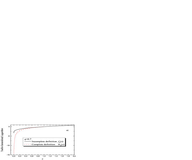
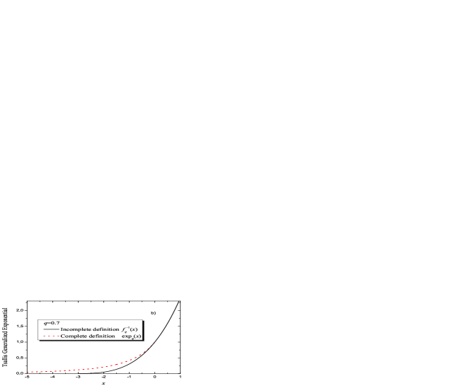
Figure 1: a) Plot of Tsallis incomplete ($f_{q}$, solid line) and complete ($\ln_{q}$, dotted line) deformed logarithm for $q=0.7$. b) Plot of Tsallis incomplete ($f^{-1}_{q}$, solid line) and complete ($\exp_{q}$, dotted line) deformed exponential for $q=0.7$.

III.1.1 Rényi entropy

One of the most discussed deformed entropic structures introduced first within information theory and then as a possible generalization of Boltzmann-Gibbs thermostatistics is the one defined by Rényi Renyi1970 ; LenziMendesSilva

$$S_{r}=\frac{1}{1-r}\ln\left(\sum_{i}p_{i}^{r}\right)$$ (16)

where $r$ is the deformation parameter and $S_{r\rightarrow 1}=S_{\mathrm{BG}}$. It has been previously shown that it exhibits a well-defined concavity only for $r\in(0,1)$ R-Concavity . The nonconcavity of the Rényi entropy outside the aforementioned range has been frequently used as an argument for the inappropriateness of the $S_{r}$-definition as a candidate for BG-generalization.

BG-entropy can be derived, without appealing to physical laws, by considering the asymptotic behavior of the Ordinary Multinomial Coefficients (OMC). The OMC gives the number of all possible configurations – or (micro)states in physics – created from the combination of objects without repetitions. In a recent study Oikonomou07 , one of the present authors (TO) constructed properly defined Deformed Multinomial Coefficients (DMC), based on the concept of the deformation parameters, in order to derive Tsallis, Rényi and nonextensive Gaussian Oik2006a entropies. Demanding the positivity of DMC, since a negative number of configuration is senseless, it has been demonstrated that Rényi entropy is defined only for $r\in(0,1)$. The same result about the parameter validity range is obtained in Ref. BagciTirnakli by applying Jaynes’ formalism for $S_{r}$ with ordinary (in contrast to the escort) exponentially averaged constraints in accordance with the fundamental mathematical structure of the Rényi entropy.

We now want to derive the interval of concavity in a more fundamental way following a different path, related to the parameter range in Eq. (14) and the definitions given by Eq. (15). In Ref. Oikonomou07 , it has been established that Rényi entropy can be expressed through the deformed multiplication introduced in Ref. Borges04 within Tsallis statistics [$x\otimes_{r}y:=\exp_{r}(\ln_{r}(x)+\ln_{r}(y))$, $x,y>1$] as follows

$$S_{r}=\ln\left(\sideset{}{{}_{\otimes_{r}}}{\prod}_{i}\left(1/p_{i}\right)^{\otimes_{r}^{p_{i}}}\right),\qquad\sideset{}{{}_{\otimes_{r}}}{\prod}_{i}\left(1/p_{i}\right)^{\otimes_{r}^{p_{i}}}=\exp_{r}\left(\sum_{i}p_{i}\ln_{r}(1/p_{i})\right)=\left[\sum_{i}p_{i}^{r}\right]^{\frac{1}{1-r}}.$$ (17)

Assuming that the deformed functions in Eq. (17) are complete, we see that the $\ln_{r}$-argument takes values in $\mathbb{L}_{1}$ (i.e., the microprobabilities vary between zero and one), and thus the $\exp_{r}$-argument varies in the interval $\mathbb{R}_{0}^{+}$. It becomes then evident that the deformation parameter $r$ takes values in $(0,1)$ as a consequence of the mathematical definition of the generalized functions in Eq. (15). Accordingly, Rényi entropy is concave for all values of its parameter range, when the complete deformed functions are being used instead of the incomplete ones. However, the very fact that one uses the complete generalized functions restricts the parameter range only to values in the interval $(0,1)$. Once we use the complete deformed functions rather than the incomplete ones, the interval of the concavity coincides with the interval of the parameter range.

III.2 Kaniadakis $\kappa$–functions

Mathematically, a very interesting case is represented by the one parametric ($\boldsymbol{\xi}=\{\xi_{1}\}=:\kappa$ with $\kappa_{0}=0$) generalization introduced by Kaniadakis Kaniadakis02 ; KaniadQuaratiScarf ; Kaniadakis05 . It is based on the following deformed functions

$$f_{\kappa}(x):=\frac{x^{\kappa}-x^{-\kappa}}{2\kappa},\qquad h_{\kappa}(x):=\Big{[}\sqrt{1+\kappa^{2}x^{2}}+\kappa x\Big{]}^{1/\kappa}$$ (18)

with $f_{\kappa}:\mathbb{R}^{+}\longrightarrow\mathbb{R}$ and $h_{\kappa}:\mathbb{R}\longrightarrow\mathbb{R}^{+}$ for $\forall\kappa\in\mathbb{R}$. Then, since $f\circ h=\mathrm{id}_{\mathbb{R}}$ and $h\circ f=\mathrm{id}_{\mathbb{R}^{+}}$, $h$ is the inverse of $f$ for all allowed values of $x$ and $\kappa$ i.e., $h_{\kappa}\equiv f^{-1}_{\kappa}$. The peculiarity of the $\kappa$–functions is that they satisfy simultaneously Eqs. (1) and (2) as well as the relations

$$f_{\kappa}(x)=-f_{\kappa}(1/x)\qquad\Leftrightarrow\qquad f^{-1}_{\kappa}(x)f^{-1}_{\kappa}(-x)=1.$$ (19)

It can be easily verified that a transformation $x\rightarrow 1/x$ of the $\kappa$-logarithmic argument or a transformation $x\rightarrow-x$ of the $\kappa$-exponential argument in Eq. (19) holds the respective relation unaltered, $\kappa=\tilde{\kappa}$ and $d_{k=1}(\kappa)=\tilde{d}_{k=1}(\tilde{\kappa})$. This means that the Kaniadakis functions are $\kappa$-symmetric and thus they preserve the same parameter (or parameter range) in their domains as well as in their codomains. The definitions in Eq. (18) are the only ones known up to now in literature which present the aforementioned property. The same result is obtained using the formalism in Section II. Assuming the expressions in Eq. (19) are not valid, we can still look for a function $d_{k=1}\equiv d:\mathcal{A}_{\kappa}\longrightarrow\mathcal{B}_{\kappa}\equiv\mathcal{B}^{(1)}_{\kappa}$ such that

$$f_{\kappa}(x)=-f_{d(\kappa)}(1/x)\qquad\Leftrightarrow\qquad f^{-1}_{\kappa}(x)f^{-1}_{d(\kappa)}(-x)=1.$$ (20)

From Eqs. (18) and (20), we determine the form of $d$ as

$$d(\kappa) =-\kappa.$$ (21)

Comparing the $\kappa$- and $d(\kappa)$-structure of $f$ and $f^{-1}$ we obtain (see the criterion of completeness i.e., Eq. (9))

$$f_{d(\kappa)}(*)=f_{\kappa}(*)\qquad\Leftrightarrow\qquad f^{-1}_{d(\kappa)}(*)=f^{-1}_{\kappa}(*),$$ (22)

where * represents any argument of $f$ or $f^{-1}$. Accordingly, the assumption does not hold and the relations in Eq. (19) are indeed satisfied. From Eq. (10) and the relation $d(\mathcal{A}_{\kappa})=\mathcal{B}_{\kappa}$ we are able to determine the $\kappa$- and $d(\kappa)$-interval given as follows

$$\mathcal{A}_{\kappa}:=[0,1),\qquad\mathcal{B}_{\kappa}:=(-1,0].$$ (23)

Eq. (22) implies that the functions in Eq. (18) are $\kappa$–symmetric, they exhibit the same image for $\kappa$ and $d(\kappa)$. Thus, whether we make use of interval $\mathcal{A}_{\kappa}$ or of interval $\mathcal{B}_{\kappa}$, we obtain the same result. In Fig. 2, we demonstrate this behavior letting the deformation parameter $\kappa$ vary in the united range $(-1,1)=\mathcal{B}_{\kappa}\bigcup\mathcal{A}_{\kappa}=d(\mathcal{A}_{\kappa})\bigcup\mathcal{A}_{\kappa}$ for $x=2$ and $1/x=2$. We note that the intervals $\mathcal{A}_{\kappa}$ and $\mathcal{B}_{\kappa}$ in Eq. (23) are identical with the ones obtained from the normalization of $1/f^{-1}_{\kappa}(x)$ and $f^{-1}_{\kappa}(-x)$, respectively.

As a result of the above discussion, we accomplish the definitions in Eq. (18) with the following information

$$f_{\kappa}\equiv\ln_{\kappa} :\mathbb{R}^{+}\longrightarrow\mathbb{R}\qquad\mathrm{with}\qquad\kappa\in\mathcal{A}_{\kappa}\vee\kappa\in\mathcal{B}_{\kappa},$$ (24a)

$$f^{-1}_{\kappa}\equiv\exp_{\kappa} :\mathbb{R}\longrightarrow\mathbb{R}^{+}\qquad\mathrm{with}\qquad\kappa\in\mathcal{A}_{\kappa}\vee\kappa\in\mathcal{B}_{\kappa}.$$ (24b)

As can be seen, the domain and the codomain of $f_{\kappa}$ and $f^{-1}_{\kappa}$ are completely analogous to the undeformed ones i.e., $\ln$ and $\exp$, respectively. In Ref. Kaniadakis02 , Kaniadakis showed that these deformed functions exhibit similar behaviors as the ordinary, undeformed functions for all boundary values of $\mathbb{R}$ and $\mathbb{R}^{+}$.

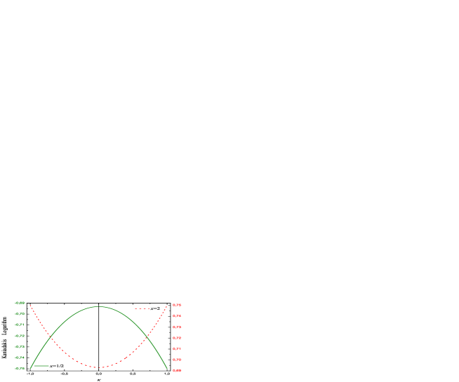
Figure 2: Plot of Kaniadakis logarithm with regard to the deformation parameter $\kappa$ in the interval $\mathcal{A}_{\kappa}\bigcup\mathcal{B}_{\kappa}=(-1,0]\bigcup[0,1)$ for $x=2$ (dotted, right axis) and $x=1/2$ (solid, left axis).

III.3 Abe $q$–logarithm

Abe’s one-parameter generalized logarithmic function ($\boldsymbol{\xi}=\{\xi_{1}\}=:q$ with $q_{0}=1$) Abe97 reads

$$f_{q}(x):=\frac{x^{1/q-1}-x^{q-1}}{1/q-q},\qquad\qquad h_{q}(x):=f^{-1}_{q}(x)$$ (25)

with $f_{q\rightarrow 1}(x)=\ln(x)$ and $h_{q\rightarrow 1}(x)=\exp(x)$. The $q$-exponential function is not analytically invertible for all allowed values of $q$. Similar to the Tsallis case, the current definition is incomplete since $f_{q}(x)\neq-f_{q}(1/x)$ with $\Theta_{q}(x)=\frac{x^{1/q-1}-x^{q-1}+x^{1-1/q}-x^{1-q}}{1/q-q}$. Concerning its domain and codomain, we obtain

$$q>0 \qquad f_{q}:\mathbb{R}^{+}\longrightarrow\mathbb{R},$$ (26a)

$$q<0 \qquad f_{q}:\mathbb{R}^{+}\longrightarrow\mathbb{R}_{0}^{-},$$ (26b)

$$q=0 \qquad f_{q}:(0,1]\bigcup(1,\infty)\longrightarrow 0\bigcup\infty.$$ (26c)

We observe an implicit dependence of the codomains on the deformation parameter in the equation above, in contrast to the explicit parameter dependence in Tsallis case. The peculiarity of Abe’s definition is that there exists a parameter variation range ($q>0$), where the codomain is identified with the one of the ordinary logarithm ($q=1$). However, one should be aware that this property does not imply completeness of $f_{q}(x)$ for $q>0$, since $\Theta_{q}(x)\neq 0$ (see the third setback in Section II).

The validity range of the deformation parameter is calculated through the conditions in Eq. (10), which yields

$$\mathcal{A}_{q}:=(1/2,1]\bigcup[1,2).$$ (27)

The duality relations are determined from Eqs. (6) and (25)

$$d_{1}(q) =\frac{q}{2q-1},\qquad d_{2}(q)=2-q.$$ (28)

The existence of two dual functions, $f_{q}(x)=-f_{d_{1}(q),d_{2}(q)}(1/x)$, depending on the same deformation parameter implies that Abe’s logarithm issues from a structure which consists primarily of two different parameters (see next subsection).

Having explicitly obtained the dual mapping function $d(q)$ and the range of validity of the deformation parameter $q$, we can now give the definition of Abe’s complete $q$-generalized functions

$$\ln_{q}(x):=\begin{cases}\displaystyle\frac{x^{1-1/q}-x^{1-q}}{q-1/q},&x\in\mathbb{L}_{0}\\ \\ \displaystyle\frac{x^{1/q-1}-x^{q-1}}{1/q-q},&x\in\mathbb{L}_{1}\end{cases}\,,\qquad\qquad\exp_{q}(x):=\begin{cases}f^{-1}_{d_{1}(q),d_{2}(q)}(x),&x\in\mathbb{R}^{-}\\ \\ f^{-1}_{q}(x),&x\in\mathbb{R}_{0}^{+}\end{cases}\,,$$ (29)

in accordance with Eq. (8).

In Fig. 3, we plot the incomplete (solid lines) and complete (dashed lines) $q$-generalized logarithms in Eqs. (25) and (29) for $q=0.6$, respectively. Both functions tend to minus infinity when $x\rightarrow 0$, which is justified through their (co)domain. However, $\ln_{q}$ decays smoother to $-\infty$ than $f_{q}$ for $0<x<1$. The complete and incomplete $q$-logarithms exhibit the same behavior for $x\geq 1$ as expected, since they are defined as a mapping from the same domain to the same codomain.

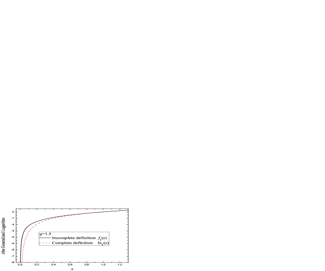
Figure 3: Plot of Abe’s incomplete ($f_{q}$, solid line) and complete ($\ln_{q}$, dotted line) deformed logarithm, for $q=1.5$.

III.4 Borges-Roditi two-parametric logarithm

A two-parameter ($\boldsymbol{\xi}=\{\xi_{1},\xi_{2}\}$ with $\xi_{1_{0}}=0=\xi_{2_{0}}$) incomplete generalization introduced by Borges and Roditi (BR) BorgesRoditi reads

$$f_{\xi_{1},\xi_{2}}(x):=\frac{x^{\xi_{1}}-x^{\xi_{2}}}{\xi_{1}-\xi_{2}},\qquad\qquad h_{\xi_{1},\xi_{2}}(x):=f^{-1}_{\xi_{1},\xi_{2}}(x)$$ (30)

with $f_{\xi_{1_{0}},\xi_{2_{0}}}(x)=\ln(x)$, $h_{\xi_{1_{0}},\xi_{2_{0}}}(x)=\exp(x)$ and $\Theta_{\xi_{1},\xi_{2}}(x)=\frac{x^{\xi_{1}}-x^{\xi_{2}}+x^{-\xi_{1}}-x^{\xi_{2}}}{\xi_{1}-\xi_{2}}$. The generalized exponential function $h_{\xi_{1},\xi_{2}}$ is not analytically invertible for all values of the deformation parameters. Concerning the domain and codomain of $f_{\xi_{1},\xi_{2}}$, we observe

$$\xi_{1},\xi_{2}>0 \qquad f_{\xi_{1},\xi_{2}}:\mathbb{R}_{0}^{+}\longrightarrow[0,\infty),\qquad\qquad\;\>\,h_{\xi_{1},\xi_{2}}:[0,\infty)\longrightarrow\mathbb{R}^{+}_{0},$$ (31a)

$$\xi_{1},\xi_{2}<0 \qquad f_{\xi_{1},\xi_{2}}:\mathbb{R}^{+}\longrightarrow(-\infty,0],\qquad\quad\;\;\>\,h_{\xi_{1},\xi_{2}}:(-\infty,0]\longrightarrow\mathbb{R}^{+},$$ (31b)

$$\xi_{1}>0,\xi_{2}=0 \qquad f_{\xi_{1},\xi_{2}}:\mathbb{R}^{+}_{0}\longrightarrow(-1/\xi_{1},\infty],\qquad\;\;\>h_{\xi_{1},\xi_{2}}:(-1/\xi_{1},\infty]\longrightarrow\mathbb{R}^{+}_{0},$$ (31c)

$$\xi_{1}<0,\xi_{2}=0 \qquad f_{\xi_{1},\xi_{2}}:\mathbb{R}^{+}\longrightarrow(-\infty,-1/\xi_{1}],\qquad h_{\xi_{1},\xi_{2}}:(-\infty,-1/\xi_{1}]\longrightarrow\mathbb{R}^{+},$$ (31d)

$$\begin{subarray}{c}\displaystyle\mathrm{sgn}(\xi_{1})\neq\mathrm{sgn}(\xi_{2})\\ \displaystyle\xi_{1}=0=\xi_{2}\end{subarray} \qquad f_{\xi_{1},\xi_{2}}:\mathbb{R}^{+}\longrightarrow\mathbb{R},\qquad\qquad\qquad\;\>\,h_{\xi_{1},\xi_{2}}:\mathbb{R}\longrightarrow\mathbb{R}^{+}.$$ (31e)

The results in Eqs. (31c) and (31d) are analogous for $\xi_{1}=0,\xi_{2}\gtrless 0$. In Eq. (31) it becomes evident that the complete definition, in the sense of Kanadiakis definition, of the functions $f_{\xi_{1},\xi_{2}}$ and $h_{\xi_{1},\xi_{2}}$ may be found only when $\mathrm{sgn}(\xi_{1})\neq\mathrm{sgn}(\xi_{2})$ ($\xi_{1}=0=\xi_{2}$ corresponds to the ordinary functions). We calculate the dual functions from Eqs. (6) and (30) as

$$d_{1}(\xi_{1}) =-\xi_{1},\qquad d_{2}(\xi_{2})=-\xi_{2}.$$ (32)

The conditions in Eq. (10) confines the values of the deformation parameters $\xi_{1}$ and $\xi_{2}$ into the following intervals

$$\mathcal{A}_{\xi_{\alpha}} :=(-\infty,0)\qquad\Leftrightarrow\qquad\mathcal{A}_{\xi_{\beta}}:=(0,1),$$ (33a)

$$\mathcal{A}_{\xi_{\alpha}} :=(0,1)\qquad\quad\,\Leftrightarrow\qquad\mathcal{A}_{\xi_{\beta}}:=(0,1),$$ (33b)

$$\mathcal{A}_{\xi_{\alpha}} :=[0,0]\qquad\quad\;\Leftrightarrow\qquad\mathcal{A}_{\xi_{\beta}}:=[0,1),$$ (33c)

where $\alpha,\beta=1,2$ with $\alpha\neq\beta$. These results are in agreement with the ones obtained in Eq. (31) for the domain of the argument when ($\xi_{1},\xi_{2}\gtrless 0$). The boundary value, $1$, is obtained from the condition (10d).

Having explicitly obtained the dual mapping function $d(q)$ and the range of validity of the deformation parameter $q$, we can now define the complete $q$-generalized functions

$$\ln_{\xi_{1},\xi_{2}}(x):=\begin{cases}\displaystyle\frac{x^{-\xi_{1}}-x^{-\xi_{2}}}{\xi_{2}-\xi_{1}},&x\in\mathbb{L}_{0}\\ \\ \displaystyle\frac{x^{\xi_{1}}-x^{\xi_{2}}}{\xi_{1}-\xi_{2}},&x\in\mathbb{L}_{1}\end{cases}\,,\qquad\qquad\exp_{\xi_{1},\xi_{2}}(x):=\begin{cases}f^{-1}_{d_{1}(\xi_{1}),d_{2}(\xi_{2})}(x),&x\in\mathbb{R}^{-}\\ \\ f^{-1}_{\xi_{1},\xi_{2}}(x),&x\in\mathbb{R}_{0}^{+}\end{cases}\,,$$ (34)

in accordance with Eq. (8).

A special feature of BR-logarithmic structure is that it includes all three deformed logarithmic definitions we have studied in this section. It can be verified that for $\{\xi_{1}=1-q,\,\xi_{2}=0\}$, $\{\xi_{1}=\kappa=-\xi_{2}\}$ and $\{\xi_{1}=1/q-1,\,\xi_{2}=q-1\}$, one obtains Tsallis, Kaniadakis and Abe logarithms, respectively. Indeed, the properties of BR-function reproduce the ones of the aforementioned functions. Thus, the BR generalized logarithms can be characterized as a family of deformed logarithms. Considering the $\Theta_{\xi_{1},\xi_{2}}$-function, we observe that the BR-logarithmic family includes only one possible structure which is complete and analytic in all points of its domain, namely, when $\xi_{2}=-\xi_{1}$, which implies $\Theta_{\xi_{1},\xi_{2}}(x)=0$, as expected. This corresponds to the Kanadiakis definition.

IV Conclusions

The recent generalizations of Boltzmann-Gibbs Statistics are based on the introduction of some deformed forms of the ordinary logarithmic and exponential functions, where $\boldsymbol{\xi}=\{\xi_{i}\}_{i=1,\ldots,u}$ denotes the deformation parameter set. It is hence of great importance to understand the mathematical structure of these deformed functions in order to gain more insight into the associated generalization schemes. Motivated by this fact, we first demonstrated that the generalized logarithms $f_{\boldsymbol{\xi}}$ (and their inverse i.e., generalized exponentials $h_{\boldsymbol{\xi}}$) are non-bijective from $\mathbb{R}^{+}$ ($\mathbb{R}$) to $\mathbb{R}$ ($\mathbb{R}^{+}$). Thus, the generalized logarithm definitions $f_{\boldsymbol{\xi}}$ may represent the inversion of the generalized exponentials $h_{\boldsymbol{\xi}}$ and vice versa, only in some subsets of $\mathbb{R}^{+}$ and $\mathbb{R}$. Therefore, they are called incomplete deformed functions. This feature issues from the non-additive $\boldsymbol{\xi}$-logarithmic and non-multiplicative $\boldsymbol{\xi}$-exponential composition rules i.e., $f_{\boldsymbol{\xi}}(xy)\neq f_{\boldsymbol{\xi}}(x)+f_{\boldsymbol{\xi}}(y)$ and $h_{\boldsymbol{\xi}}(x+y)\neq h_{\boldsymbol{\xi}}(x)h_{\boldsymbol{\xi}}(y)$. The incompleteness of deformed functions is not only a mathematical deficiency, but also presents some physical problems, since it restricts the applicability of the associated thermostatistics. In other words, it is the incomplete mathematical structure, which dictates the range of arguments or results, rather than the physical system one studies. However, the estimation of the aforementioned subsets is not a trivial procedure, since some boundary values present $x(\boldsymbol{\xi})$-dependence. In order to overcome this difficulty and to guarantee the property of bijectivity in the original (co)domains, we proposed dual mapping functions $d_{k}(\boldsymbol{\xi})$ ($k=1,\ldots,v\geqslant u$), which enable a change of the parameters within specific subsets of $\mathbb{R}^{+}$ and $\mathbb{R}$. Through the introduction of such dual functions, one is able to obtain bijective deformed functions, $\ln_{\boldsymbol{\xi}}$ and $\exp_{\boldsymbol{\xi}}$, which are called complete. If $\mathcal{A}_{\boldsymbol{\xi}},\,\mathcal{B}^{(k)}_{\boldsymbol{\xi}}\subseteq\mathbb{R}$ are parameter ranges related over a function $d_{k}:\mathcal{A}_{\boldsymbol{\xi}}\rightarrow\mathcal{B}^{(k)}_{\boldsymbol{\xi}}$ such that $f_{\boldsymbol{\xi}}(x)=-f_{d_{k}(\boldsymbol{\xi})}(1/x)$ and $h_{\boldsymbol{\xi}}(x)=1/h_{d_{k}(\boldsymbol{\xi})}(-x)$, then for $\boldsymbol{\xi}\in\mathcal{A}_{\boldsymbol{\xi}}\;(d_{k}(\boldsymbol{\xi})\in\mathcal{B}^{(k)}_{\boldsymbol{\xi}})$, the complete deformed functions are defined in the following domains and codomains, $\ln_{\boldsymbol{\xi}}:\{f_{d_{k}(\boldsymbol{\xi})}(x),\>x\in(0,1]\}\bigcup\{f_{\boldsymbol{\xi}}(x),\>x\in[1,\infty)\}$ $\longrightarrow$ $\{f_{d_{k}(\boldsymbol{\xi})}(x)\in(-\infty,0]\}\bigcup\{f_{\boldsymbol{\xi}}(x)\in[0,\infty)\}$ and $\exp_{\boldsymbol{\xi}}:\{h_{d_{k}(\boldsymbol{\xi})}(x),\>x\in(-\infty,0]\}\bigcup\{h_{\boldsymbol{\xi}}(x),\>x\in[0,\infty)\}$ $\longrightarrow$ $\{h_{d_{k}(\boldsymbol{\xi})}(x)\in(0,1]\}\bigcup\{h_{\boldsymbol{\xi}}(x)\in[1,\infty)\}$, with $h_{\boldsymbol{\xi}}\equiv f^{-1}_{\boldsymbol{\xi}}$ and $h_{d_{k}(\boldsymbol{\xi})}\equiv f^{-1}_{d_{k}(\boldsymbol{\xi})}$. Further, we posited conditions that the generalized logarithmic and exponential functions have to fulfill in order to preserve the main properties of their ordinary counterparts e.g., the behavior at the boundary points and the points of extrema. Through these conditions, we determine the ranges $\mathcal{A}_{\boldsymbol{\xi}}$ and $\mathcal{B}^{(k)}_{\boldsymbol{\xi}}$.

Concerning the dual functions $d_{k}(\boldsymbol{\xi})$, we formulated a criterion to distinguish between deformed logarithmic/exponential structures which are bijective in the original (co)domains, preserving the same parameter for all values of the argument, and those whose bijectivity is assured in the intervals presented above.

The application of our theoretical formalism to Tsallis $q$-definitions led to the parameter ranges $\mathcal{A}_{q}=(0,1]$ and $\mathcal{B}_{q}^{(1)}=[1,2)$ connected to one another through the dual function $d(q)=2-q$. Moreover, writing the Rényi entropy in terms of Tsallis deformed functions, we have obtained the interval of concavity associated with Rényi entropy by the estimation of the parameter range resulted from the criterion of completeness.

Similarly, we considered Kaniadakis generalized functions and derived the parameter intervals $\mathcal{A}_{\kappa}=[0,1)$ and $\mathcal{B}^{(1)}_{\kappa}=(-1,0]$ connected through the dual function $d(\kappa)=-\kappa$. However, Kaniadakis generalizations satisfy, in complete analogy to the ordinary functions, the identities $f_{\kappa}(x)=-f_{\kappa}(1/x)$ and $f^{-1}_{\kappa}(x)=1/f^{-1}_{\kappa}(-x)$, revealing their $\kappa$-symmetric structure. Due to this property of Kaniadakis generalized functions, the introduction of the dual function is unnecessary. Indeed, we verify that the $\kappa$- and $d(\kappa)$-structure of $f$ or $f^{-1}$ are identical. In this case, the aforementioned deformed maps preserve the same parameter values in their entire domain and codomain. The existence of two parameter ranges $\mathcal{A}_{\kappa}$ and $\mathcal{B}^{(1)}_{\kappa}$ is not in contradiction with the latter statement, since the $\kappa$-symmetric generalizations give the same image whether $\kappa\in\mathcal{A}_{\kappa}$ or $d(\kappa)\in\mathcal{B}^{(1)}_{\kappa}$.

Our final applications were Abe and Borges-Roditi deformed functions. In each case, we were able to determine the respective parameter intervals and the duality functions. Since the Borges-Roditi generalization scheme includes all three deformed logarithmic (and deformed exponential) definitions i.e., Tsallis, Kaniadakis and Abe deformed functions, the compact form of the dual function and the parameter intervals associated with it were found to reduce to those of the Tsallis, Kaniadakis and Abe deformed functions by identifying $\{\xi_{1}=1-q,\,\xi_{2}=0\}$, $\{\xi_{1}=\kappa=-\xi_{2}\}$ and $\{\xi_{1}=1/q-1,\,\xi_{2}=q-1\}$, respectively. The Borges-Roditi logarithmic family includes only one possible complete and analytic structure in all points of its domain, namely, when $\xi_{2}=-\xi_{1}$. This corresponds to the Kaniadakis generalization scheme.

It is worth noting that the criterion of completeness developed here is not an alternative to the generalized sum or product rules. Although these generalized algebras may help preserve some properties of the ordinary exponential and logarithmic functions, they are nevertheless defined in terms of generalized functions. Therefore, they too suffer from the incompleteness of the deformed functions. Moreover, the criterion of completeness is far more general than the approach of generalized algebras, since the latter may drastically change from one generalization to the other. The criterion of completeness, on the other hand, is always based on the same procedure i.e., calculating the dual functions and the valid parameter intervals.

The current results unveil new perspectives on the consideration of generalized logarithmic and exponential functions, thereby shedding light on various mathematical aspects in need of revision and proper treatment.

References

• (1) C. Tsallis, Possible Generalization of Boltzmann–Gibbs Statistics, J. Stat. Phys. 521/2 (1988) 479.
• (2) G. Kaniadakis, Statistical mechanics in the context of special relativity, Phys. Rev. E 66, 056125 (2002).
• (3) E.P. Borges, I. Roditi, A family of nonextensive entropies Physics Letters A 246, 399 (1998).
• (4) S. Abe, A note on the $q$-deformation-theoretic aspect of the generalized entropies in nonextensive physics, Phys. Lett. A 224 (1997) 326.
• (5) A. Rényi, Probability theory, Amsterdam: North-Holland, 1970.
• (6) C. Tsallis, Introduction to onextensive statistical mechanics: approaching a complex world, New York: Springer, 2009.
• (7) G. Kaniadakis, P. Quarati P & A.M. Scarfone, Kinetical foundations of non-conventional statistics, Physica A 305(1), 76 (2002).
• (8) G. Kaniadakis, M. Lissia and A.M. Scarfone, Two-parameter deformations of logarithm, exponential, and entropy: A consistent framework for generalized statistical mechanics, Phys. Rev. E 71, 046128 (2005).
• (9) Th. Oikonomou, U. Tirnakli, Generalized entropic structures and non-generality of Jaynes’ Formalism, Chaos Solitons & Fractals, accepted (2009).
• (10) A. M. Teweldeberhan, A. R. Plastino and H. G. Miller, On the cut-off prescriptions associated with power-law generalized thermostatistics, Phys. Lett. A 343 (2005) 71.
• (11) E.K. Lenzi, R.S. Mendes & L.R. da Silva, Statistical mechanics based on Renyi entropy, Physica A 280, 337 (2000).
• (12) J.D. Rahmshaw, Thermodynamic stability conditions for the Tsallis and Rényi entropies, Phys. Lett. A 198 (1995) 119; C. Tsallis, Comment on “Thermodynamic stability conditions for the Tsallis and Renyi entropies” by J.D. Ramshaw, Phys. Lett. A 206 (1995) 389; G.R. Guerberoff, G.A. Raggio, Remarks on “Thermodynamic stability conditions for the Tsallis and Re’nyi entropies” by Ramshaw , Phys. Lett. A 214 (1996) 313.
• (13) Th. Oikonomou, Tsallis, Rényi and nonextensive Gaussian entropy derived from the respective multinomial coefficients, Physica A 386 (2007) 119.
• (14) Th. Oikonomou, Properties of the “nonextensive” Gaussian entropy, Physica A 381 (2007) 155.
• (15) G. B. Bagci, U. Tirnakli, On the way towards a generalized entropy maximization procedure, Arxiv:0811.4564v1, (2008).
• (16) E.P. Borges, A possible deformed algebra and calculus inspired in nonextensive thermostatistics, Physica A 340 (2004) 95; L. Nivanen, A. Le Mehaute & Q.A. Wang, Generalized algebra within a nonextensive statistics, Rep. Math. Phys. 52 (2003) 437.