Unstable Anisotropic Loop Quantum Cosmology

Abstract

We study stability conditions of the full Hamiltonian constraint equation describing the quantum dynamics of the diagonal Bianchi I model in the context of LQC. Our analysis has shown robust evidence of an instability in the explicit implementation of the difference equation, implying important consequences for the correspondence between the full LQG theory and LQC. As a result, one may question the choice of the quantisation approach, the model of lattice refinement, and/or the rôle of the ambiguity parameters; all these should in principle be dictated by the full LQG theory.

I Introduction

Loop Quantum Gravity (LQG) rovelli2004 is a non-perturbative, background independent, canonical quantisation of General Relativity in four space-time dimensions. Even though the full theory of LQG is not yet complete, its successes encourage the application of LQG techniques to mini-superspaces obtained by a symmetry reduction. The application of LQG to the cosmological sector is known as Loop Quantum Cosmology (LQC) Ashtekar:2003hd ; Bojowald:2002gz . In the homogeneous and isotropic cosmological models with a massless scalar field, which plays the rôle of an internal time parameter according which other physical quantities “evolve”, quantum geometry effects of the full LQG theory lead to a repulsive force in the Planckian regime. Thus, the big bang singularity is resolved and replaced by a quantum bounce Ashtekar:2006wn . The underlying discreteness of LQC is the key element for the existence of the quantum bounce; similar results have thus been also obtained in the context of other models.

LQC quantum dynamics are determined by a difference, rather than a differential, equation, as a result of quantum geometry effects. However, such effects can be neglected as one departs from the Planckian regime, and quantum dynamics can then be well approximated by the Wheeler-DeWitt (WDW) differential equation. LQC is formulated in terms of SU(2) holonomies of the connection and triads. In the “old” quantisation, the quantised holonomies were taken to be shift operators with a fixed magnitude, but later it was found that this leads to problematic instabilities in the continuum semi-classical limit, where the WDW wave-function becomes a good approximation to the difference equation of LQC. In a dynamical equation closer to what is expected to be obtained from the full LQG theory, lattice refinement would take place during the evolution, since full Hamiltonian constraint operators generally create new vertices of a lattice state in addition to changing their edge labels. The effect of the refinement of the discrete lattice has been modelled and the elimination of the instabilities in the continuum era has been explicitly shown Nelson:2007um ; Nelson:2007wj ; Nelson:2008vz . Lattice refinement leads to new dynamical difference equations which, in general, do not have a uniform step-size making their study quite involved. In contrast to isotropic models, which can be understood in terms of wave-functions on a one-dimensional discrete mini-superspace, anisotropic models with higher-dimensional mini-superspaces, can be more subtle. For the partial difference equations of anisotropic models, stability issues can turn out to be more serious than in isotropic ones, leading to consistency tests, and thus restricting possible quantisation freedom. In Ref. Nelson:2008bx we have proposed a numerical method, based on Taylor expansions, which provides the necessary information to calculate the wave-function at any given lattice point. We have developed Nelson:2008bx numerical schemes for both the one-dimensional homogeneous and isotropic cosmological case, which has analytic solutions, as well as the two-dimensional case of a Schwarszchild interior, which cannot be exactly solved.

LQC issues of the Bianchi type I models, the simplest among anisotropic cosmologies, have been also investigated. Besides their simplicity, such models are very interesting for addressing the issue of space-like singularities in the context of the full LQG theory. As in the isotropic case, a massless scalar field plays the rôle of an internal time parameter. Recent analysis Ashtekar:2009vc has shown that the big bang singularity is solved by quantum gravity effects, while LQC dynamics is well approximated by that of the WDW theory once quantum geometry effects become negligible.

The aim of this paper is to analyse the stability conditions of the solutions to the full Hamiltonian constraint. Unstable (i.e., growing) solutions would indicate unphysical spurious solutions, for which there is no correspondence between the difference (valid in the LQC regime) and the differential (WDW) equations. This would indicate an inconsistency between the full LQG theory and the mini-superspace LQC approach, implying the possibility of a weakness of the employed quantisation approach. This work is organised as follows: In Section II we outline the basic formalism of LQG and LQC. In Section III we perform a stability analysis. We summarise our results and we discuss the outcome of our findings in Section IV.

II Basics of the LQG/LQC formalism

Let us restrict ourselves to diagonal Bianchi I metrics, for which space-time metric in Cartesian coordinates, $\tau,x_{i}$ (i=1,2,3), reads

$${\rm d}s^{2}=-N^{2}{\rm d}\tau^{2}+\sum_{i=1}^{3}a_{i}^{2}{\rm d}x_{i}^{2}~{},$$ (1)

where $N$ is the lapse function and $a_{i}$ (with $i=1,2,3$) stand for the three directional scale factors. Following Ref. Ashtekar:2009vc we choose $\tau$ to satisfy $\Box\tau=0$.

LQG/LQC are based on a Hamiltonian formulation of General Relativity, with basic variables an SU(2) valued connection $A^{i}_{a}$ and the conjugate momentum variable which is a densitised triad $E^{a}_{i}$ , a derivative operator quantised in the full LQG theory in the form of fluxes. As for any quantisation scheme based on a Hamiltonian framework or an action principle, for the homogeneous flat model one should regularise the divergences which appear due to the homogeneity as the action and Hamiltonian are integrated over spatial hyper-surfaces. We thus restrict spatial homogeneity and Hamiltonian to an elementary cell ${\cal V}$, which we choose so that its edges lie along the fixed coordinate axis $x_{i}$ (with $i=1,2,3$). In addition, we fix a fiducial flat metric ${}^{0}q_{ab}$, with line element

$${\rm d}s_{0}^{2}=\sum_{i=1}^{3}{\rm d}x_{i}^{2}~{}.$$ (2)

The lengths of the three edges of the elementary cell ${\cal V}$ and its volume, as measured by the fiducial flat metric ${}^{0}q_{ab}$, are denoted by $L_{i}$ (with $i=1,2,3$) and $V_{0}=L_{1}L_{2}L_{3}$, respectively.

The densitised triad carries information about the spatial geometry, encoded in the three-metric, while the connection carries information about the spatial curvature, in the form of the spin-connection and the extrinsic curvature. We introduce physical triads ${}^{0}e^{a}_{i}$ and their dual (${{}^{0}}e^{a}_{i}\ {}^{0}\omega^{j}_{a}=\delta^{j}_{i}$) co-triads ${}^{0}\omega^{i}_{a}=D_{a}x^{i}$, satisfying ${}^{0}q_{ab}={{}^{0}}\omega^{i}_{a}\ {}^{0}\omega^{j}_{b}\delta_{ij}$. Note that $i$ refers to the Lie algebra index and $a$ is a spatial index with $a,i=1,2,3$. The physical co-triads are given by $\omega^{a}_{i}=a^{i}\ {{}^{0}}\omega^{i}_{a}$, and the physical three-metric by $q_{ab}=\omega^{i}_{a}\omega^{j}_{b}\delta_{ij}$.

The six-dimensional phase space is defined through the SU(2) connection $A^{i}_{a}$ and the triad $E^{a}_{i}$ given by

$$A^{i}_{a} = c^{i}(L^{i})^{-1}\ {{}^{0}}\omega^{i}_{a}$$

$$E^{a}_{i} = p_{i}L_{i}V_{o}^{-1}\sqrt{{}^{0}q}\ {{}^{0}}e^{a}_{i}~{},$$ (3)

where the connection components $c_{i}$ and the momenta $p_{i}$ are constants; $q=(p_{1}p_{2}p_{3})^{0}qV_{0}^{-1}$ stands for the determinant of the physical spatial metric $q_{ab}$. The three momenta $p_{i}$ are related to the three scale factors through

$$p_{1} = {\rm sgn}(a_{1})|a_{2}a_{3}|L_{2}L_{3}$$

$$p_{2} = {\rm sgn}(a_{2})|a_{1}a_{3}|L_{1}L_{3}$$

$$p_{3} = {\rm sgn}(a_{3})|a_{1}a_{2}|L_{1}L_{2}~{}.$$ (4)

The pairs $c^{i},p_{i}$ (with $i=1,2,3$) satisfy the Poisson brackets relations:

$$\{c^{i},p_{j}\}=8\pi G\gamma\delta^{i}_{j}~{},$$ (5)

with $\gamma$ the Barbero-Immirzi parameter.

Two of the constraints of the full LQG theory, namely the Gauss and the diffeomorphism constraints are identically satisfied and one is therefore left with the Hamiltonian constraint, as for the isotropic case. Restricting the integration to the fiducial cell ${\cal V}$, the Hamiltonian constraint reads

$${\cal C}=\int_{\cal V}N({\cal H}_{\rm grav}+{\cal H}_{\rm matter}){\rm d}^{3}x~{},$$ (6)

where ${\cal H}_{\rm grav}$ and ${\cal H}_{\rm matter}$ stand for the gravitational and the matter parts of the constraint densities, respectively. The lapse function $N$ is $N=\sqrt{|p_{1}p_{2}p_{3}|}$.

Since Bianchi I models are spatially flat, the matter part of the Hamiltonian constraint can be written as Ashtekar:2009vc

$${\cal H}_{\rm grav}=-{\sqrt{{}^{0}q}\over 8\pi G\gamma^{2}\sqrt{p_{1}p_{2}p_{3}}V_{0}}(p_{1}p_{2}c_{1}c_{2}+p_{1}p_{3}c_{1}c_{3}+p_{2}p_{3}c_{2}c_{3})~{}.$$ (7)

The matter part of the Hamiltonian constraint is Ashtekar:2009vc

$${\cal H}_{\rm matter}=\sqrt{q}\rho_{\rm matter}~{},$$ (8)

where $\rho_{\rm matter}$ is the matter energy density of the matter field, chosen to be a massless scalar field $T$;

$$\rho_{\rm matter}={p^{2}_{T}\over 2|p_{1}p_{2}p_{3}|}~{},$$ (9)

with $p_{T}$ the canonically conjugate momentum of $T$. The scalar field $T$ can be considered as an evolution parameter in the classical theory, and as a viable internal time parameter in the subsequent quantum theory. The justification for this choice lies in the fact that since $p_{T}$ is a constant of motion, $T$ grows linearly in time $\tau$, for any solution to the field equations. The full Hamiltonian constraint, Eq. (7) can then be finally written as Ashtekar:2009vc

$${\cal H}=-{1\over 8\pi G\gamma^{2}}(p_{1}p_{2}c_{1}c_{2}+p_{1}p_{3}c_{1}c_{3}+p_{2}p_{3}c_{2}c_{3})+{p_{T}^{2}\over 2}~{}.$$ (10)

Let us proceed with the quantum kinematics of Bianchi I LQC. The gravitational part of the kinematic Hilbert space, ${\cal H}_{\rm kin}^{\rm grav}$, can be expressed in the momentum, $p_{i}$ (with $i=1,2,3$), representation. Given an orthonormal basis states $|p_{1},p_{2},p_{3}\rangle$, which are eigenstates of quantum geometry, consider a linear combination

$$|\Psi\rangle=\sum_{p_{1},p_{2},p_{3}}\Psi(p_{1},p_{2},p_{3})|p_{1},p_{2},p_{3}\rangle~{},$$ (11)

with finite norm, namely

$$\sum_{p_{1},p_{2},p_{3}}|\Psi(p_{1},p_{2},p_{3})|^{2}<\infty~{},$$ (12)

and

$$\langle p_{1},p_{2},p_{3}|p^{\prime}_{1},p^{\prime}_{2},p^{\prime}_{3}\rangle=\delta_{p_{1}p_{1}^{\prime}}\delta_{p_{2}p_{2}^{\prime}}\delta_{p_{3}p_{3}^{\prime}}~{}.$$ (13)

The action of the elementary operators, which are the three momenta $p_{i}$ (with $i=1,2,3$) and the holonomies $h_{i}^{(\ell)}$ along edges parallel to the three axis $x_{i}$ (with $i=1,2,3$) — completely determined by almost periodic ($\ell$ is any real number) functions $\exp(i\ell c_{j})$ of the connection — is given by Ashtekar:2009vc

$$\hat{p}_{1}|p_{1},p_{2},p_{3}\rangle = p_{1}|p_{1},p_{2},p_{3}\rangle$$

$$\widehat{\exp(i\ell c_{1})}|p_{1},p_{2},p_{3}\rangle = |p_{1}-8\pi G\gamma\hbar\ell,p_{2},p_{3}\rangle~{},$$ (14)

and similarly for $\hat{p}_{2},\widehat{\exp(i\ell c_{2})}$ and $\hat{p}_{3},\widehat{\exp(i\ell c_{3})}$.

One has then to build the quantum analogue of the Hamiltonian constraint, along the lines of the isotropic case. To do so, one has to find the operator on the gravitational sector of the kinematic Hilbert space, corresponding to the curvature $F_{ab}^{\ \ k}$ of the connection $A^{i}_{a}$, given by

$$F_{ab}^{\ \ k}=2\partial_{[a}A_{b]}^{\ \ k}+\epsilon_{ij}^{\ \ k}A^{i}_{a}A^{j}_{b}~{}.$$ (15)

As it is known from the isotropic case, the connection operator does not exist in LQG/LQC; we cannot take the limit of the area enclosed by a plaquette to go to zero, since the minimum area enclosed by the plaquette is the nonzero eigenvalue $\Delta p_{\rm Pl}^{2}$ (with $\Delta$ a dimensionless number, $\Delta=4\sqrt{3}\pi\gamma$) of the area operator. To single out a unique plaquette of the many ones enclosing an area $\Delta p_{\rm Pl}^{2}$ on each of the three faces of the elementary cell ${\cal V}$, we will use the natural gauge fixing available for the diagonal Bianchi I case, and a correspondence between kinematic states in LQG and LQC. In this way, one obtains that the curvature operator reads Ashtekar:2009vc

$$\hat{F}_{ab}^{\ \ k}=\epsilon_{ij}^{\ \ k}\left({\sin{\bar{\mu}c}\over\bar{\mu}L}\ ^{0}\omega_{a}\right)^{i}\left({\sin{\bar{\mu}c}\over\bar{\mu}L}\ ^{0}\omega_{b}\right)^{j}~{},$$ (16)

where

$$\left({\sin{\bar{\mu}c}\over\bar{\mu}L}\ ^{0}\omega_{a}\right)^{i}={\sin{\bar{\mu}}^{i}c^{i}\over{\bar{\mu}}^{i}L^{i}}\ ^{0}\omega^{i}_{a}~{},$$ (17)

with

$$\bar{\mu}_{1} = \sqrt{{|p_{1}|\Delta l^{2}_{\rm Pl}\over|p_{2}p_{3}|}}~{},$$

$$\bar{\mu}_{2} = \sqrt{{|p_{2}|\Delta l^{2}_{\rm Pl}\over|p_{1}p_{3}|}}~{},$$

$$\bar{\mu}_{3} = \sqrt{{|p_{3}|\Delta l^{2}_{\rm Pl}\over|p_{1}p_{2}|}}~{}.$$ (18)

The functional dependence of $\bar{\mu}_{i}$ on $p_{i}$ is essential since otherwise quantum dynamics can depend on the choice of the fiducial cell ${\cal V}$.

Consequently, one can now write the quantum analogue of the full Hamiltonian constraint, Eq. (6). It reads Ashtekar:2009vc

$$-\hbar^{2}\partial_{T}^{2}\Psi(\vec{\lambda},T)=\Theta\Psi(\vec{\lambda},T)~{},$$ (19)

where $\Theta=-{\cal C}_{\rm grav}$.

To simplify the gravitational sector of the Hamiltonian constraint, one can introduce the volume of the elementary cell ${\cal V}$ as one of the arguments of the wave function. Let us then set Ashtekar:2009vc

$$\nu=2\lambda_{1}\lambda_{2}\lambda_{3}~{},$$ (20)

which is directly related to the volume of ${\cal V}$, namely

$$\hat{V}\Psi(\lambda_{1},\lambda_{2},\nu)=2\pi|\gamma|\sqrt{\Delta}|\nu|l^{3}_{\rm pl}\Psi(\lambda_{1},\lambda_{2},\nu)~{},$$ (21)

with $\gamma={\rm sgn}(p_{1}p_{2}p_{3})|\gamma|$. Thus, the new configuration variables will be $\lambda_{1},\lambda_{2},\nu$.

In the next section, we will write out explicitly the full Hamiltonian constraint and we will then study the stability of its solutions.

III Stability analysis

The basic difference equation arising from the loop quantisation of the Bianchi I model reads Ashtekar:2009vc

$$\partial_{T}^{2}\Psi\left(\lambda_{1},\lambda_{2},\nu;T\right) = \frac{\pi G}{2}\sqrt{\nu}\Bigl{[}\left(\nu+2\right)\sqrt{\nu+4}\Psi^{+}_{4}\left(\lambda_{1},\lambda_{2},\nu;T\right)-\left(\nu+2\right)\sqrt{\nu}\Psi^{+}_{0}\left(\lambda_{1},\lambda_{2},\nu;T\right)$$ (22)

$$-\left(\nu-2\right)\sqrt{\nu}\Psi^{-}_{0}\left(\lambda_{1},\lambda_{2},\nu;T\right)+\left(\nu-2\right)\sqrt{|\nu-4|}\Psi^{-}_{4}\left(\lambda_{1},\lambda_{2},\nu;T\right)\Bigr{]}~{},$$

where

$$\Psi^{+}_{4}\left(\lambda_{1},\lambda_{2},\nu;T\right) = \sum_{i\neq j=(0,1,2)}\Psi\left(a_{i}\lambda_{1},a_{j}\lambda_{2},\nu+4;T\right)$$

$$\Psi^{-}_{4}\left(\lambda_{1},\lambda_{2},\nu;T\right) = \sum_{i\neq j=(-3,-2,0)}\Psi\left(a_{i}\lambda_{1},a_{j}\lambda_{2},\nu-4;T\right)$$

$$\Psi^{+}_{0}\left(\lambda_{1},\lambda_{2},\nu;T\right) = \sum_{i\neq j=(-1,0,1)}\Psi\left(a_{i}\lambda_{1},a_{j}\lambda_{2},\nu;T\right)$$

$$\Psi^{-}_{0}\left(\lambda_{1},\lambda_{2},\nu;T\right) = \sum_{i\neq j=(-2,0,3)}\Psi\left(a_{i}\lambda_{1},a_{j}\lambda_{2},\nu;T\right)~{},$$ (23)

and the functions $a_{i}$ have been defined as follows:

$$a_{-3}\equiv\left(\frac{\nu-4}{\nu-2}\right)~{},\ \ \ a_{-2}\equiv\left(\frac{\nu-2}{\nu}\right)~{},\ \ \ a_{-1}\equiv\left(\frac{\nu}{\nu+2}\right)~{},$$

$$a_{0}\equiv 1~{},\ \ \ a_{1}\equiv\left(\frac{\nu+4}{\nu+2}\right)~{},\ \ \ a_{2}\equiv\left(\frac{\nu+2}{\nu}\right)~{},\ \ \ a_{3}\equiv\left(\frac{\nu}{\nu-2}\right)~{}.$$ (24)

Numerical evolution can in principle be carried out by restricting to the positive octant ($\lambda_{1}\geq 0,\lambda_{2}\geq 0,\nu\geq 0$), thus eliminating the ${\rm sgn}(\lambda_{i})$ factors which are otherwise appearing in various terms.

Here we wish to examine the stability of the vacuum solutions, in which case the solution is static, namely $\Psi\left(\lambda_{1},\lambda_{2},\nu;T\right)=\Psi\left(\lambda_{1},\lambda_{2},\nu\right)$, and Eq. (22) becomes

$$\Psi^{+}_{4}\left(\lambda_{1},\lambda_{2},\nu\right)=\sqrt{\frac{\nu}{\nu+4}}\Psi^{+}_{0}\left(\lambda_{1},\lambda_{2},\nu\right)+\left(\frac{\nu-2}{\nu+2}\right)\sqrt{\frac{\nu}{\nu+4}}\Psi^{-}_{0}\left(\lambda_{1},\lambda_{2},\nu\right)-\left(\frac{\nu-2}{\nu+2}\right)\sqrt{\frac{|\nu-4|}{\nu+4}}\Psi^{-}_{4}\left(\lambda_{1},\lambda_{2},\nu\right)~{},$$ (25)

for $\nu\neq 0$; otherwise the above equation must be multiplied by $\sqrt{\nu}$, thus corresponding to the classical singularity. The geometry of this difference equation is drawn in Fig. 1. Equation (25) can be used to evaluate the value of the wave-function on the $\nu+4$ plane, given suitable boundary conditions on the $\nu$ and $\nu-4$ planes. The requirement that the arguments must be positive (i.e., $\lambda_{1}\geq 0$, $\lambda_{2}\geq 0,\nu\geq 0$) reduces the required number of boundary conditions. For the purpose of our work, it is sufficient to consider starting from a plane in which $\nu-4>0$.

In addition to specifying the boundary conditions on the $\nu$ and $\nu-4$ planes, we are also required to specify the value at five of the points given in $\Psi^{+}_{4}\left(\lambda_{1},\lambda_{2},\nu\right)$. There are in total $23$ values that are required and with such initial data the difference equation, Eq. (22), can be used to evaluate the $24^{\rm th}$ point. Once this point has been evaluated, it can be used to “move” the central point and evaluate the wave-function at subsequent positions in the $\nu+4$ plane. In this way the difference equation can be used to find the wave-function that is consistent with the Hamiltonian constraint, Eq. (22), and the boundary conditions. In principle, this procedure can be iterated to evaluate the consistent wave-function for all subsequent $\nu$-planes, however the stability of the difference equation can be investigated even at this first iteration.

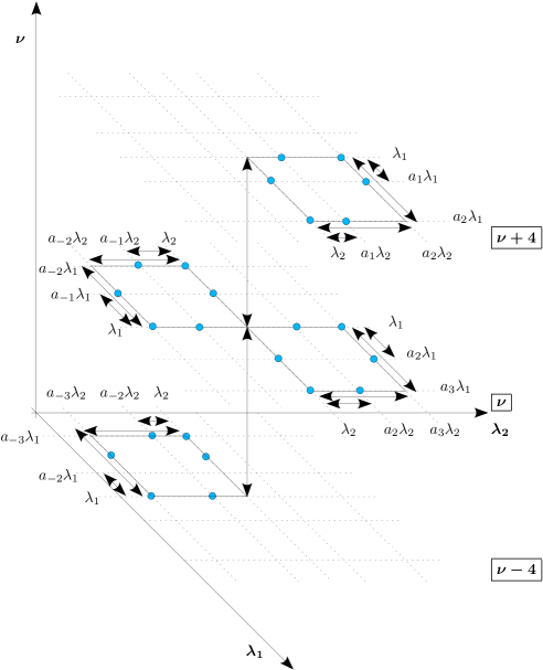
Figure 1: The geometry of the points used in the difference equation that results from the Hamiltonian constraint, for the Bianchi I model.

As shown in Fig. 1, there is a choice to be made as to which point in the $\nu+4$ plane is to be calculated from the difference equation. This choice amounts to deciding whether to increase $\lambda_{1}$ or $\lambda_{2}$ first, when populating the $\nu+4$ plane. From the point of view of the plane, the difference equation, Eq. (22), can be seen as progressively evaluating the wave-function at points first along either the $\lambda_{1}$ direction or the $\lambda_{2}$ one (see, Fig. 2). In this sense, we can consider Eq. (22) as an “evolution” equation of a wave-function with respect to either $\lambda_{1}$ or $\lambda_{2}$, subject to suitable boundary conditions. It is important to realise however that this “evolution” has only to do with the order in which the points are evaluated and is not related, in any way, to evolution of the wave-function with respect to time.

With this view, standard von Neumann stability analysis can be preformed on Eq. (22), to see if the system is stable Bojowald:2003dn ; Rosen:2006bga . Here however caution is necessary. Von Neumann’s analysis is typically used to see if there are growing mode solutions to a particular discretised version of an underlying differential equation. In this case, the difference equation is the fundamental evolution equation, which can be approximated by a differential equation (the anisotropic Wheeler-DeWitt equation Ashtekar:2009vc ) in a suitable limit. In standard numerical implementations of differential equations, the stability of the system is important only because artificial numerical rounding errors can grow to dominate the behaviour of the solution, however the situation here is very different. In principle, the difference equation, Eq. (22), is exact and hence all solutions should be considered, however in practise we wish to restrict only to those solutions that closely approximate General Relativity at large scales. This makes the use of von Neumann stability analysis useful, since we are comparing a particular difference equation, with the differential equation it approximates, however it is important to remember that the motivation is very different than in standard numerical analysis.

For homogeneous and isotropic cosmologies, a local stability analysis of the corresponding difference equation to determine the behaviour of spurious solutions was performed in Ref. Vandersloot:2005kh , using higher order spin $J$ representations of the holonomies for the quantisation. It was found Vandersloot:2005kh that the use of higher spin holonomies to regulate the gravitational part of the constraint operator leads to modifications, which are qualitatively similar to those of the inverse scale factor. Stability analysis has shown that the $J=1$ difference equation is not locally stable. To further determine whether these spurious solutions represent a problem with the quantisation, the authors of Ref. Vandersloot:2005kh have studied the physical inner product, since unphysical solutions would have either vanishing or infinite physical norm and would be modded out of the physical Hilbert space. For the cases of Bianchi I locally rotationally symmetric cosmology and that of the Schwarzschild interior geometry, a von Neumann stability analysis of a difference equation obtained by a previous quantisation approach was carried out in Ref. Rosen:2006bga , where there were identified large regions in space-time that have generically instabilities. In what follows, we will look for spurious solutions to Eq. (22), in the sense that they do not approximate solutions to the relevant Wheeler-DeWitt equation in the large volume limit.

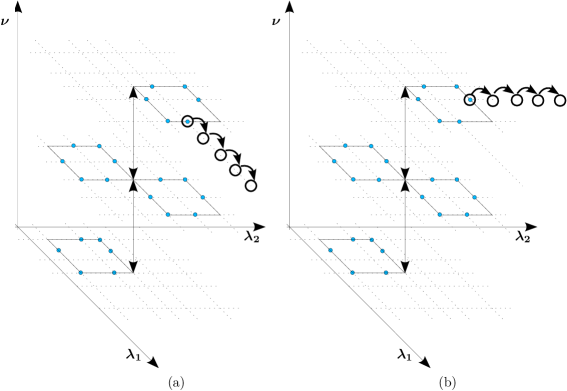
Figure 2: The difference equation gives us a point in the $\nu+4$ plane, given the required $23$ points. Exactly which point is calculated via the difference equation is somewhat arbitrary and essentially describes the way in which the $\nu+4$ plane is calculated. In the l.h.s. scheme (a) the point $\left(a_{2}\lambda_{1},a_{1}\lambda_{2},\nu+4\right)$ is calculated, in which case the $\nu+4$ plane is evaluated first along constant $\lambda_{2}$. In the r.h.s. scheme (b) the point chosen is $\left(a_{1}\lambda_{1},a_{2}\lambda_{2},\nu+4\right)$ and the $\nu+4$ plane would be evaluated first along constant $\lambda_{1}$.

As in standard von Neumann stability analysis, we will decompose the solutions of the difference equation, Eq. (25), into Fourier modes and look for growing modes. Specifically, we consider the ansatz

$$\Psi\left(\lambda_{1},\lambda_{2},\nu\right)=T\left(\lambda_{1}\right)\exp\left(i\left(\omega\lambda_{2}+\chi\nu\right)\right)~{},$$ (26)

where we have chosen the $\lambda_{1}$ direction to be the direction in which the $\nu+4$ plane is “evolved”. Using the above ansatz, Eq. (25) becomes

$$e^{4\chi i}\sum_{i\neq j=\left(0,1,2\right)}T\left(a_{i}\lambda_{1}\right)e^{i\left(\omega a_{j}\lambda_{2}+\chi\nu\right)} = \sqrt{\frac{\nu}{\nu+4}}\sum_{i\neq j=\left(-1,0,1\right)}T\left(a_{i}\lambda_{1}\right)e^{i\left(\omega a_{j}\lambda_{2}+\chi\nu\right)}$$

$$+\left(\frac{\nu-2}{\nu+2}\right)\sqrt{\frac{\nu}{\nu+4}}\sum_{i\neq j=\left(-2,0,3\right)}T\left(a_{i}\lambda_{1}\right)e^{i\left(\omega a_{j}\lambda_{2}+\chi\nu\right)}$$

$$-\left(\frac{\nu-2}{\nu+2}\right)\sqrt{\frac{|\nu-4|}{\nu+4}}e^{-4\chi i}\sum_{i\neq j=\left(-3,-2,0\right)}T\left(a_{i}\lambda_{1}\right)e^{i\left(\omega a_{j}\lambda_{2}+\chi\nu\right)}~{}.$$

To simplify each of the summations, we proceed as follows:

$$\sum_{i\neq j=\left(-1,0,1\right)}T\left(a_{i}\lambda_{1}\right)e^{i\omega\lambda_{2}} = T\left(a_{1}\lambda_{1}\right)\left(e^{i\omega\lambda_{2}}+e^{i\omega a_{-1}\lambda_{2}}\right)$$ (28)

$$+~{}T\left(a_{0}\lambda_{1}\right)\left(e^{i\omega a_{-1}\lambda_{2}}+e^{i\omega a_{1}\lambda_{2}}\right)$$

$$+~{}T\left(a_{-1}\lambda_{1}\right)\left(e^{i\omega a_{1}\lambda_{2}}+e^{i\omega\lambda_{2}}\right)~{},$$

which becomes

$$\sum_{i\neq j=\left(-1,0,1\right)}T\left(a_{i}\lambda_{1}\right)e^{i\omega\lambda_{2}} = 2e^{i\omega\lambda_{2}}\Biggl{[}T\left(a_{1}\lambda_{1}\right)e^{-\frac{i\omega\lambda_{2}\left(a_{1}-1\right)}{2}}\cos\left(\frac{\omega\lambda_{2}\left(a_{1}-1\right)}{2}\right)$$ (29)

$$\ \ \ \ \ \ \ \ \ \ +T\left(a_{0}\lambda_{1}\right)\cos\left(\omega\lambda_{2}\left(a_{1}-1\right)\right)$$

$$\ \ \ \ \ \ \ \ \ \ +T\left(a_{1}\lambda_{1}\right)e^{\frac{i\omega\lambda_{2}\left(a_{1}-1)\right)}{2}}\cos\left(\frac{\omega\lambda_{2}\left(a_{1}-1\right)}{2}\right)\Biggr{]}~{},$$

where we made use that

$$a_{-3}-1=-\left(a_{3}-1\right)~{},\ \ \ a_{-2}-1=-\left(a_{2}-1\right)~{},\ \ \ a_{-1}-1=-\left(a_{1}-1\right)~{}.$$ (30)

We can simplify the other summations in a similar way.

Explicitly putting in the values of $a_{1},a_{2},a_{3}$ given in Eq. (III), the difference equation, Eq. (III), becomes

$$e^{4\chi i}\Biggl{[}T\left(a_{0}\lambda_{1}\right)e^{\frac{2i\omega\lambda_{2}\left(\nu+1\right)}{\nu\left(\nu+2\right)}}\cos\left(\frac{2\omega\lambda_{2}\left(\nu+1\right)}{\nu\left(\nu+2\right)}\right)+T\left(a_{1}\lambda_{1}\right)e^{\frac{i\omega\lambda_{2}}{v}}\cos\left(\frac{\omega\lambda_{2}}{\nu}\right)$$

$$\ \ \ \ \ \ \ \ +T\left(a_{2}\lambda_{1}\right)e^{\frac{i\omega\lambda_{2}}{\nu+2}}\cos\left(\frac{\omega\lambda_{2}}{\nu+2}\right)\Biggr{]}$$

$$=\ \sqrt{\frac{\nu}{\nu+4}}\Biggl{[}T\left(a_{-1}\lambda_{1}\right)e^{\frac{-i\omega\lambda_{2}}{\nu+2}}\cos\left(\frac{\omega\lambda_{2}}{\nu+2}\right)+T\left(a_{0}\lambda_{1}\right)\cos\left(\frac{2\omega\lambda_{2}}{\nu+2}\right)$$

$$\ \ \ \ \ \ \ \ \ \ \ \ \ \ \ \ \ \ +T\left(a_{1}\lambda_{1}\right)e^{\frac{i\omega\lambda_{2}}{\nu+2}}\cos\left(\frac{\omega\lambda_{2}}{\nu+2}\right)\Biggr{]}$$

$$\ \ -\left(\frac{\nu-2}{\nu+2}\right)\sqrt{\frac{\nu}{\nu+4}}\Biggl{[}T\left(a_{-2}\lambda_{1}\right)e^{\frac{i\omega\lambda_{2}}{\nu-2}}\cos\left(\frac{\omega\lambda_{2}}{\nu-2}\right)+T\left(a_{0}\lambda_{1}\right)e^{\frac{2i\omega\lambda_{2}}{\nu\left(\nu-2\right)}}\cos\left(\frac{2\omega\lambda_{2}}{\nu\left(\nu-2\right)}\right)$$

$$\ \ \ \ \ \ \ \ \ \ \ \ \ \ \ \ \ \ \ \ \ \ \ \ \ \ \ \ \ \ \ +T\left(a_{3}\lambda_{1}\right)e^{\frac{i\omega\lambda_{2}}{\nu}}\cos\left(\frac{\omega\lambda_{2}}{\nu}\right)\Biggr{]}$$

$$\ \ -\left(\frac{\nu-2}{\nu+2}\right)\sqrt{\frac{|\nu-4|}{\nu+4}}e^{-4\chi i}\Biggl{[}T\left(a_{-3}\lambda_{1}\right)e^{\frac{-i\omega\lambda_{2}}{\nu}}\cos\left(\frac{\omega\lambda_{2}}{\nu}\right)+T\left(a_{-2}\lambda_{1}\right)e^{\frac{-i\omega\lambda_{2}}{\nu-2}}\cos\left(\frac{\omega\lambda_{2}}{\nu-2}\right)$$

$$\ \ \ \ \ \ \ \ \ \ \ \ \ \ \ \ \ \ \ \ \ \ \ \ \ \ \ \ \ \ \ \ \ \ \ \ \ \ \ +T\left(a_{0}\lambda_{1}\right)e^{\frac{-i\omega\lambda_{2}\left(\nu-1\right)}{\nu\left(\nu-2\right)}}\cos\left(\frac{\omega\lambda_{2}\left(\nu-1\right)}{\nu\left(\nu-2\right)}\right)\Biggr{]}~{}.$$ (31)

Up to this point the equation is exact, however expanding in terms of small $1/\nu$, Eq. (III) becomes

$$e\left(4\chi\right)\Biggl{[}T\left(a_{0}\lambda_{1}\right)e\left(2\Lambda\right)\cos\left(2\Lambda\right)+\left(T\left(a_{1}\lambda_{2}\right)+T\left(a_{2}\lambda_{1}\right)\right)e\left(\Lambda\right)\cos\left(\Lambda\right)\biggr{]}$$

$$=\left\{1-\frac{2}{\nu}\right\}\Biggl{[}T\left(a_{0}\lambda_{1}\right)\cos\left(2\Lambda\right)+T\left(a_{-1}\lambda_{1}\right)e\left(-\Lambda\right)\cos\left(-\Lambda\right)+T\left(a_{1}\lambda_{1}\right)e\left(\Lambda\right)\cos\left(\Lambda\right)\Biggr{]}$$

$$+\left(1-\frac{6}{\nu}\right)\Biggl{[}T\left(a_{-2}\lambda_{1}\right)e\left(-\Lambda\right)\cos\left(-\Lambda\right)+T\left(a_{3}\lambda_{1}\right)e\left(\Lambda\right)\cos\left(\Lambda\right)\Biggr{]}$$

$$-\left\{1-\frac{8}{\nu}\right\}e\left(-4\chi\right)\Biggl{[}T\left(a_{-3}\lambda_{1}\right)e\left(-\Lambda\right)\cos\left(-\Lambda\right)+T\left(a_{-2}\lambda_{1}\right)e\left(-\Lambda\right)\cos\left(-\Lambda\right)+T\left(a_{0}\lambda_{1}\right)e\left(-\Lambda\right)\cos\left(-\Lambda\right)\Biggr{]}$$

$$+{\cal O}\left(\frac{1}{\nu^{2}}\right)~{},$$ (32)

where we have defined the function

$$e\left(x\right)=e^{ix}~{},$$ (33)

and the variable

$$\Lambda=\omega\lambda_{2}/\nu~{}.$$ (34)

Equation (III) can be re-ordered to read

$$AT\left(a_{3}\lambda_{1}\right)=BT\left(a_{2}\lambda_{1}\right)+CT\left(a_{1}\lambda_{1}\right)+DT\left(a_{0}\lambda_{1}\right)+ET\left(a_{-1}\lambda_{1}\right)+FT\left(a_{-2}\lambda_{1}\right)+GT\left(a_{-3}\lambda_{1}\right)~{},$$ (35)

where

$$A = -\left[1-\frac{6}{\nu}\right]e\left(\Lambda\right)\cos\left(\Lambda\right)$$

$$B = -e\left(4\chi\right)e\left(\Lambda\right)\cos\left(\Lambda\right)$$

$$C = \left[1-\frac{2}{\nu}-e\left(4\chi\right)\right]e\left(\Lambda\right)\cos\left(\Lambda\right)$$

$$D = \left[-e\left(4\chi\right)e\left(2\Lambda\right)+1-\frac{2}{\nu}\right]\cos\left(2\Lambda\right)-\left[1-\frac{8}{\nu}\right]e\left(-4\chi\right)e\left(-\Lambda\right)\cos\left(-\Lambda\right)$$

$$E = \left[1-\frac{2}{\nu}\right]e\left(-\Lambda\right)\cos\left(-\Lambda\right)$$

$$F = \left[1-\frac{6}{\nu}-\left\{1-\frac{8}{\nu}\right\}e\left(-4\chi\right)\right]e\left(-\Lambda\right)\cos\left(-\Lambda\right)$$

$$G = -\left[1-\frac{8}{\nu}\right]e\left(-4\chi\right)e\left(-\Lambda\right)\cos\left(-\Lambda\right)~{}.$$ (36)

Equation (35) is equivalent to the vector equation

$$M_{1}\overline{T}_{3}=M_{2}\overline{T}_{2}~{},$$ (37)

where we have defined the vectors

$$\overline{T}_{i}=\left[\begin{array}[]{c}T\left(a_{i}\lambda_{1}\right)\\ T\left(a_{i-1}\lambda_{1}\right)\\ T\left(a_{i-2}\lambda_{1}\right)\\ T\left(a_{i-3}\lambda_{1}\right)\\ T\left(a_{i-4}\lambda_{1}\right)\\ T\left(a_{i-5}\lambda_{1}\right)\end{array}\right]~{}~{}\mbox{for}~{}~{}i=2,3$$ (38)

and the matrices

$$M_{1}=\left(\begin{array}[]{cccccc}A&0&0&0&0&0\\ 0&1&0&0&0&0\\ 0&0&1&0&0&0\\ 0&0&0&1&0&0\\ 0&0&0&0&1&0\\ 0&0&0&0&0&1\end{array}\right)~{},\ \ \ \ \ M_{2}=\left(\begin{array}[]{cccccc}B&C&D&E&F&G\\ 1&0&0&0&0&0\\ 0&1&0&0&0&0\\ 0&0&1&0&0&0\\ 0&0&0&1&0&0\\ 0&0&0&0&1&0\end{array}\right)~{}.$$ (39)

Stability of this system is then given by the eigenvalues of the matrix $\left(M_{1}\right)^{-1}M_{2}$. More particularly, if

$$\max|\tilde{\lambda}|\leq 1~{}~{}~{}\forall~{}~{}\omega\ \mbox{and}\ \chi~{},$$ (40)

where $\tilde{\lambda}$ are the eigenvalues of the matrix $\left(M_{1}\right)^{-1}M_{2}$, then the amplitude $T\left(a_{3}\lambda_{1}\right)$ is less than that of previous points, namely the difference equation is stable.

One finds, in block form, that

$$\left(M_{1}\right)^{-1}M_{2}=\left(\begin{array}[]{c|c}\tilde{A},\tilde{B},\tilde{C},\tilde{D},\tilde{E}&\tilde{F}\\ \hline\cr\mathbbm{1}_{5}&\underline{0}_{5}\end{array}\right)~{},$$ (41)

where $\mathbbm{1}_{5}$ is the $5\times 5$ identity matrix, $\underline{0}_{5}$ is the zero vector and

$$\tilde{A} = \left[1+\frac{6}{\nu}\right]e\left(4\chi\right)$$

$$\tilde{B} = -\left[1+\frac{6}{\nu}\right]\left[1-\frac{2}{\nu}-e\left(4\chi\right)\right]$$

$$\tilde{C} = \left[1+\frac{6}{\nu}\right]\left[e\left(4\chi\right)e\left(2\Lambda\right)+1-\frac{2}{\nu}\right]e\left(-\Lambda\right)\frac{\cos\left(2\Lambda\right)}{\cos\left(\Lambda\right)}+\left[1-\frac{2}{\nu}\right]e\left(-4\chi\right)$$

$$\tilde{D} = -\left[1+\frac{4}{\nu}\right]e\left(-2\Lambda\right)$$

$$\tilde{E} = -\left[1+\frac{6}{\nu}\right]\left[1-\frac{6}{\nu}-\left\{1-\frac{8}{\nu}\right\}e\left(-4\chi\right)\right]e\left(-2\Lambda\right)$$

$$\tilde{F} = \left[1-\frac{2}{\nu}\right]e\left(-4\chi\right)e\left(-2\Lambda\right)~{},$$ (42)

with $e(x)$ as defined in Eq. (33), previously. The eigenvalues of Eq. (41) are found by solving the characteristic equation

$$\Big{|}\left(M_{1}\right)^{-1}M_{2}-\tilde{\lambda}\mathbbm{1}_{6}\Big{|}=0~{},$$ (43)

for the eigenvalues $\tilde{\lambda}$; note that $\mathbbm{1}_{6}$ is the $6\times 6$ identity matrix. We are looking for the maximum $|\tilde{\lambda}|$, for all $\omega$ and $\chi$. We can immediately see that the system will not be stable, since the inverse of $M_{1}$ only exists when $|A|\neq 0$. The cases when $|A|=0$ correspond to

$$\Lambda=\frac{\left(2n-1\right)\pi}{2}~{},$$ (44)

or, equivalently, using Eq. (34):

$$\omega=\frac{\left(2n-1\right)\pi}{2}\frac{\nu}{\lambda_{2}}~{},$$ (45)

with $n\in\mathbb{Z}$ and these modes are explicitly unstable. This can be understood by noting that the amplitude $T\left(a_{3}\lambda_{1}\right)$ is multiplied by $A$, which can be made arbitrarily small, hence then the amplitude $T\left(a_{3}\lambda_{1}\right)$ has to be arbitrarily large.

We can go further and consider the $0^{\rm th}$ order limit in the $(1/\nu)\rightarrow 0$ expansion, in which the definitions given in Eq. (III) simplify to

$$\tilde{A}^{(0)} = e^{4i\chi}$$

$$\tilde{B}^{(0)} = -\left(1-e^{4i\chi}\right)$$

$$\tilde{C}^{(0)} = \left(e^{4i\chi+2i\Lambda}+1\right)e^{-i\Lambda}\frac{\cos 2\Lambda}{\cos\Lambda}+e^{-4i\chi}$$

$$\tilde{D}^{(0)} = -e^{-2i\Lambda}$$

$$\tilde{E}^{(0)} = -\left(1-e^{-4i\chi}\right)e^{-2i\Lambda}$$

$$\tilde{F}^{(0)} = e^{-4i\chi-2i\Lambda}~{},$$ (46)

where the superscript ⁽⁰⁾, reminds us that we are working to the $0^{\rm th}$ order in the small $(1/\nu)$ expansion.

If we further consider the modes given by $\Lambda=\pi/4$ and $\chi=0$, then the above coefficients, Eq. (III), become simply

$$\tilde{A}^{(0)} = 1~{},\ \ \ \ \tilde{B}^{(0)}=0~{},$$

$$\tilde{C}^{(0)} = 1~{},\ \ \ \ \tilde{D}^{(0)}=i~{},$$

$$\tilde{E}^{(0)} = 0~{},\ \ \ \ \tilde{F}^{(0)}=-i~{}.$$ (47)

In this specific case, the matrix given in Eq. (41) reads

$$M_{1}^{-1}M_{2}=\left(\begin{array}[]{cccccc}1&0&1&i&0&-i\\ 1&0&0&0&0&0\\ 0&1&0&0&0&0\\ 0&0&1&0&0&0\\ 0&0&0&1&0&0\\ 0&0&0&0&1&0\end{array}\right)~{},$$ (48)

the determinant of which is simply

$$\det\left(M_{1}^{-1}M_{2}\right)=-i~{},$$ (49)

implying

$$-i=\Pi_{j=1}^{6}\tilde{\lambda}_{j};$$ (50)

$\tilde{\lambda}_{j}$ are the eigenvalues of the matrix $M_{1}^{-1}M_{2}$. Since $|\Pi_{j=1}^{6}\tilde{\lambda}_{j}|=1$, either $\max\left(|\tilde{\lambda}_{j}|\right)>1$, or $|\tilde{\lambda}_{j}|=1,\ \forall j\ \mbox{with}\ j=1,\cdots,6$. We can rule out the second possibility by explicit evaluation of the characteristic equation, Eq. (43), for this ansatz.

To be more specific, set $\tilde{\lambda}_{j}=\exp\left(i\theta_{j}\right)$ and solve Eq. (43), subject to the limit $(1/\nu)\rightarrow 0$, for the modes $\Lambda=\pi/4$ and $\chi=0$, to find $\theta_{j}$. In this case, Eq. (43) becomes

$$-\left(1-e^{i\theta_{j}}\right)e^{5i\theta_{j}}-e^{3i\theta_{j}}-i\left(1-e^{2i\theta_{j}}\right)=0\ \ ,\forall j\ \mbox{with}\ j=1,\cdots 6~{}.$$ (51)

The above equation, Eq. (51), has only two (numeric) solutions, which without loss of generality we denote by $\theta_{1},\theta_{2}$, and are approximately equal to $\theta_{1}=1.18123$ and $\theta_{2}=2.30716$, for $\theta_{1},\theta_{2}\in\left(0,2\pi\right)$. However, using Eq. (50), the sum of the phases of the six eigenvalues must satisfy

$$\sum_{j=1}^{6}\theta_{j}=\left(2n-1\right)\pi\ \ {\rm for}\ \ n\in\mathbb{Z}~{}.$$ (52)

With only two solutions, the eigenvalues must be degenerate. Let us suppose that $|\tilde{\lambda}_{j}|=1,\ \forall j\ \mbox{with}\ j=1,\cdots,6$, and consider $p$ eigenvalues with phase $\theta_{1}$ and $q$ eigenvalues with phase $\theta_{2}$, where $p$ and $q$ are integers satisfying $p+q=6$. We can then look for any combination of degeneracies (i.e., any values of $p$ and $q$) that satisfy Eq. (52). Explicitly it can be verified that there is no such solution, which implies that not all of the eigenvalues lie on the complex unit circle and hence there must be at least one eigenvalue with $|\tilde{\lambda}_{j}|>1$.

A partial proof of this result in the general case can be produced by using a variant of the Gershgorin circle theorem Gerschgorin1 ; Gerschgorin2 . The standard theorem states that the eigenvalues of a matrix ${\cal M}=\left(a_{ij}\right)$, lie within the $i$ discs, $D\left(a_{ii},R\right)$ (called Gershgorin discs) in the complex plane with centre $a_{ii}$ and radius $R=\sum_{i\neq j}|a_{ij}|$. It can further be shown that if the discs are disjoint, then there is at least one eigenvalue within each connected region. For the case of the matrix given by Eq. (41) this implies that all of the eigenvalues lie within the discs

$$D\left(0,1\right)~{}~{},~{}~{}D\left(\tilde{A},|\tilde{B}|+|\tilde{C}|+|\tilde{D}|+|\tilde{E}|+|\tilde{F}|\right)~{}.$$ (53)

Of the two discs, the second one is the most interesting. It is centred at $\tilde{A}$ and one can easily check that for $(1/\nu)\neq 0$, it is beyond the unit complex circle, i.e., $|\tilde{A}|>1$. However, one can also check that the radius satisfies

$$|\tilde{B}|+|\tilde{C}|+|\tilde{D}|+|\tilde{E}|+|\tilde{F}|>|\tilde{A}|-1~{},$$ (54)

except for small values of $\nu$. Thus, the two Gershgorin discs intersect and we cannot say that there is an eigenvalue with $|\lambda_{j}|>1$. However, by noting that $|\tilde{C}|$ becomes arbitrarily large for $\Lambda\rightarrow\pi/2$, one realises that the radius of the second disc in Eq. (53), encompasses all of the complex plane. This would tend to suggest that there is at least one eigenvalue that is not constrained to have $|\lambda_{j}|<1$. A variation on the proof of the standard Gershgorin circle theorem can be used to show that this is indeed the case.

Consider the case of a matrix ${\cal M}=\left(a_{ij}\right)$ such that $|a_{13}|\gg\sum_{j\neq 3}|a_{1j}|$. Then the characteristic equation is

$$\sum_{j=1}^{6}a_{ij}x_{j}=\lambda x_{i}\ \ \forall i~{},$$ (55)

where $x=\left(x_{i}\right)$ is the eigenvector of ${\cal M}$ and $\lambda$ is the corresponding eigenvalue. Expanding this sum as

$$a_{i3}x_{3}+\sum_{j\neq 3}a_{ij}x_{j}=\lambda x_{i}~{},$$ (56)

gives

$$\left|\lambda-a_{i3}\frac{x_{3}}{x_{i}}\right|=\left|\sum_{j\neq 3}a_{ij}\frac{x_{j}}{x_{i}}\right|~{},$$ (57)

which is valid, provided $x_{i}\neq 0$. If we take $x_{i}$ to be

$$x_{i}=\max(x_{j})\ \ \mbox{for}\ \ j\neq 3~{},$$ (58)

we have

$$\left|\lambda-a_{i3}\frac{x_{3}}{x_{i}}\right|\leq\sum_{j\neq 3}|a_{ij}|~{}.$$ (59)

Thus, the eigenvalue $\lambda$ is within a disc, centred at the point $a_{i3}x_{3}/x_{i}$ with radius given by the sum of the magnitudes of the elements along the $i^{\rm th}$ row of ${\cal M}$, excluding the third element. In particular, if $|a_{13}|\nearrow\infty$, then for $x_{3}/x_{1}>0$, the centre of the disc tends to infinity. Provided the sum $\sum_{j\neq 3}|a_{1j}|$ remains finite, the eigenvalue $\lambda$ will lie within a disc that is entirely outside the complex unit circle and hence $|\lambda|>1$. This is precisely the situation we have for ${\cal M}=M_{1}^{-1}M_{2}$, in the case of $\Lambda\rightarrow\pi/2$.

The final element that is required for this proof is that $x_{3}/x_{1}>0$ or, more precisely, that $a_{13}x_{3}/x_{1}\gg\sum_{j\neq 3}|a_{1j}|$, given that $|a_{13}|\gg\sum_{j\neq 3}|a_{1j}|$ . In the particular case of the matrix given by Eq. (41), we can evaluate the simultaneous equations implied by the characteristic equation, Eq. (43), to find

$$\tilde{C}x_{3} \approx \lambda x_{1}~{},\ \ \ x_{1}=\lambda x_{2}~{},\ \ \ x_{2}=\lambda x_{3}~{},$$

$$x_{3} = \lambda x_{4}~{},\ \ \ x_{4}=\lambda x_{5}~{},\ \ \ x_{5}=\lambda x_{6}~{},$$ (60)

where we have used the approximation that $\tilde{C}$ dominates the terms in $\sum_{i}|a_{1i}|$. This gives

$$\left|a_{13}\frac{x_{3}}{x_{1}}\right|\approx\left|\tilde{C}\right|^{1/3}~{}.$$ (61)

Thus, provided that $\left|\tilde{C}\right|^{1/3}\gg\sum_{j\neq 3}|a_{1j}|$, the proof is valid and we have $\max\left(|\lambda_{i}|\right)>1$. Note that this condition is certainly met as $\Lambda\rightarrow\pi/2$, since $\tilde{C}$ diverges, whilst $\sum_{i}\left|a_{1i}\right|$ remains finite. This is essentially the result we preempted in the comments following Eq. (43), however here we have explicitly extended it to the case of $\tilde{C}$ large, but not infinite (i.e., the case when $M_{1}$ is invertible, but $A$ is large).

IV Conclusions

The aim of this paper is to study the stability of the Hamiltonian constraint equation valid for anisotropic Bianchi I LQC. Performing a von Neumann stability analysis, we have shown that if the difference equation admits solutions with amplitudes that grow locally, then it is not locally stable. On the one hand, this result certainly questions the validity of the quantisation, since any semi-classical solutions would quickly become dominated by the expanding spurious ones. On the other hand however, the presence of such an instability may not be, necessarily, a problem, since it might be that the unstable trajectories are explicitly removed by the physical inner product.

More precisely, the difference equation, given by Eq. (22), is unconditionally unstable. By this we mean that there is no region of $\left(\lambda_{1},\lambda_{2},\nu\right)$ in which the difference equation, Eq. (22), is stable. It is worth noting however, that in Eq. (35) we choose to re-order the difference equation in such a way that it produces a single amplitude ($T\left(a_{3}\lambda_{1}\right)$ in Eq. (35)), given the other $23$ amplitudes. This is clearly an explicit implementation of the equation. It is also possible that this difference equation could be implemented via an implicit scheme, i.e., that the equation could be re-ordered to give (say) two amplitudes, given the values of the other $23$ or $22$ amplitudes. In order for the system to give solutions, one would then have to implement consistency relations between the calculated amplitudes at different iterations. There are, of course, many ways that such an implicit implementation of the difference equation could be under taken and they could, in principle, have different stability properties.

We have demonstrated the presence of an instability in the explicit implementation of the difference equation, Eq. (22), in several ways: we have first shown that for a particular set of critical modes, $\Lambda=(2n-1)\pi/2$, the system is unstable. We have then showed that in the large $\nu$ limit, the system is again unstable for the modes $\Lambda=\pi/4$ and $\chi=0$. Finally, we have formally showed that the system is unstable for a general $\nu$, for modes that approach the critical value. This was done via a version of the Gershgorin circle theorem, which have explicitly demonstrated the instability, even for modes approaching (but not reaching) the critical value.

References

• (1) C. Rovelli, Quantum Gravity (Cambridge University Press, Cambridge, 2004).
• (2) A. Ashtekar, M. Bojowald and J. Lewandowski, Adv. Theor. Math. Phys.  7 (2003) 233 [arXiv:gr-qc/0304074].
• (3) M. Bojowald, Class. Quant. Grav.  19 (2002) 2717 [arXiv:gr-qc/0202077].
• (4) A. Ashtekar, T. Pawlowski and P. Singh, Phys. Rev.  D 74 (2006) 08400 [arXiv:gr-qc/0607039].
• (5) W. Nelson and M. Sakellariadou, Phys. Rev.  D 76 (2007) 104003 [arXiv:0707.0588 [gr-qc]].
• (6) W. Nelson and M. Sakellariadou, Phys. Rev.  D 76 (2007) 044015 [arXiv:0706.0179 [gr-qc]].
• (7) W. Nelson and M. Sakellariadou, Phys. Rev.  D 78 (2008) 024006 [arXiv:0806.0595 [gr-qc]].
• (8) W. Nelson and M. Sakellariadou, Phys. Rev.  D 78 (2008) 024030 [arXiv:0803.4483 [gr-qc]].
• (9) A. Ashtekar and E. Wilson-Ewing, Phys. Rev.  D 79 (2009) 083535 [arXiv:0903.3397 [gr-qc]].
• (10) K. Vandersloot, Phys. Rev.  D 71 (2005) 103506 [arXiv:gr-qc/0502082].
• (11) M. Bojowald and G. Date, Class. Quant. Grav.  21 (2004) 121 [arXiv:gr-qc/0307083].
• (12) J. Rosen, J. H. Jung and G. Khanna, Class. Quant. Grav.  23, 7075 (2006) [arXiv:gr-qc/0607044].
• (13) S. Gerschgorin, Izv. Akad. Nauk. USSR Otd. Fiz.-Mat. Nauk 7, 749, 1931.
• (14) Varga, R. S. Geršgorin and His Circles, Berlin, Springer-Verlag (2004).