Computational Models of Stellar Collapse and Core-Collapse Supernovae

Abstract

Core-collapse supernovae are among Nature’s most energetic events. They mark the end of massive star evolution and pollute the interstellar medium with the life-enabling ashes of thermonuclear burning. Despite their importance for the evolution of galaxies and life in the universe, the details of the core-collapse supernova explosion mechanism remain in the dark and pose a daunting computational challenge. We outline the multi-dimensional, multi-scale, and multi-physics nature of the core-collapse supernova problem and discuss computational strategies and requirements for its solution. Specifically, we highlight the axisymmetric (2D) radiation-MHD code VULCAN/2D and present results obtained from the first full-2D angle-dependent neutrino radiation-hydrodynamics simulations of the post-core-bounce supernova evolution. We then go on to discuss the new code Zelmani which is based on the open-source HPC Cactus framework and provides a scalable AMR approach for 3D fully general-relativistic modeling of stellar collapse, core-collapse supernovae and black hole formation on current and future massively-parallel HPC systems. We show Zelmani’s scaling properties to more than 16,000 compute cores and discuss first 3D general-relativistic core-collapse results.

1 Introduction

Core-collapse supernova (CCSN) explosions are powered by the release of gravitational energy in the collapse of a massive star’s core to a protoneutron star (PNS). While this general CCSN picture may be clear, its details have evaded understanding despite many decades of concerted theoretical and numerical effort.

When thermonuclear core burning ends, the core of a massive star (i.e., $M\gtrsim 8-10$ solar masses $[M_{\odot}]$) is comprised of iron-group nuclei (or O/Ne nuclei in the lowest-mass massive stars) and supported against gravity’s pull primarily by the degeneracy pressure of relativistic electrons. Shell burning adds mass to this core and eventually pushes it over its maximum supportable mass. Gravitational collapse results and is accelerated by the capture of electrons on free and bound protons and by the photodissociation of heavy nuclei into alphas and nucleons. Core collapse continues until the central, subsonically-collapsing region (the inner core of $\sim 0.5\,M_{\odot}$) reaches nuclear density. There, the strong nuclear force kicks in, stiffening the nuclear equation of state (EOS) and halting collapse, resulting in the rebound of the inner core into the still collapsing outer core. A hydrodynamic shock is formed in this core bounce and initially propagates outward in mass and radius while losing energy to the dissociation of heavy infalling nuclei and neutrinos that stream away from the postshock region. The shock stalls within $\sim 10-20\,\mathrm{ms}$ after bounce and at a radius of $\sim 100-200\,\mathrm{km}$. For a successful CCSN explosion, it must be re-energized, otherwise continued accretion will push the PNS over its mass limit. This results in a second phase of gravitational collapse, leading to the formation of a black hole, turning the stellar collapse event into a collapsar [2].

Finding and understanding the mechanism of shock revival has been the key problem of core-collapse supernova theory in the past $\sim 45+$ years. Current theory and modeling suggests (see, e.g., [3, 4] and references therein) that there are (at least) three ways to blow up massive stars: (1) the neutrino mechanism, relying primarily on an imbalance between charged-current neutrino heating and cooling in the immediate postshock regions in combination with convection and the standing-accretion-shock instability (SASI) (e.g., [5, 8, 6, 7]), (2) the magnetorotational mechanism, based on bipolar jets created by strong magnetic stresses in rapidly rotating cores (e.g., [9, 10, 11]) and (3) the acoustic mechanism recently proposed by Burrows et al. [12, 13, 14], which rests on the excitation of non-radial pulsations in the PNS by accretion and turbulence and their damping by strong sound waves that steepen into shocks, depositing energy very efficiently in the postshock region. The acoustic mechanism has not yet been confirmed by other groups and perturbative work suggests that the pulsation amplitudes may be limited by a parametric instability that transfers energy in faster damping daughter modes [15], but this mechanism remains a compelling possiblity.

In the three potential explosion mechanisms, the breaking of spherical symmetry is either fundamentally necessary or a key facilitating factor, making multi-D modeling a necessity. Furthermore, a CCSN simulation must not only spatially resolve the steep gradients at the PNS surface and the small to large scale turbulent eddies of overturn (typical $\Delta x\sim\mathcal{O}(100\,\mathrm{m})$ or less for magnetoturbulence [11, 16]), but the simulation domain must also extend to many thousand kilometers to encompass sufficient material to track a long-term postbounce accretion phase without boundary effects affecting the evolution and to allow a potential explosion to fully develop. Hence, multi-scale modeling is required and may be implemented via fixed and/or adaptive mesh refinement (FMR/AMR) or particle methods (smoothed particle hydrodynamics [SPH], e.g. [17]). Furthermore, for a complete model of stellar collapse and the CCSN postbounce phase, a broad spectrum of tightly-coupled physics must be included – ideally accurately, but at least approximately. This includes, but is not necessarily limited to, (magneto)hydrodynamics (MHD), general relativity (GR), nuclear physics (nuclear EOS and nuclear reactions), neutrino radiation-transport, and neutrino-matter interaction microphysics.

The multi-D, multi-scale, and multi-physics nature of the CCSN problem makes it complex and difficult to model and solve computationally. At the same time, however, owing to its complexity, physically accurate computational modeling, in combination with future detailed observations of CCSN neutrinos and gravitational waves, is our only chance of solving it.

In this contribution to the Scientific Discovery through Advanced Computing (SciDAC) Conference 2009, we discuss central aspects of our broad computational approach to stellar collapse and the CCSN problem and highlight recently obtained results. In section 2, we introduce the CCSN code VULCAN/2D and present results from the first long-term full-2D momentum-space angle-dependent radiation-hydrodynamics simulations of the postbounce phase in CCSNe. We go on to describe in section 3 our full-GR 3D stellar collapse simulation package Zelmani which is based on the Cactus computational framework [19] and designed for massively-parallel execution. Zelmani has already been applied to simulations of rapidly-rotating 3D core collapse for which we present results. In Section 4, we wrap up and present a forward-looking summary.

2 Angle-Dependent Neutrino Radiation-Hydrodynamic VULCAN/2D Simulations

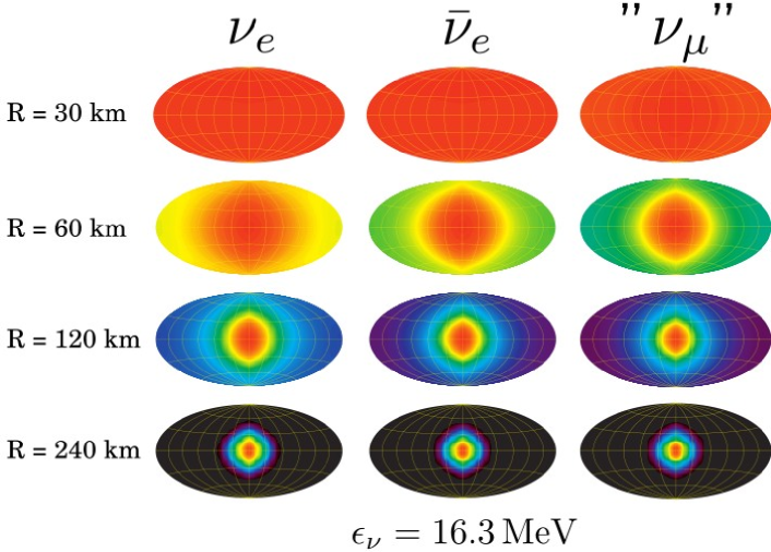
Figure 1: Hammer-type (smoothed) map projections of the normalized specific intensity $I_{\nu}(\vartheta,\varphi)/J_{\nu}$ (where $J_{\nu}$ is the mean intensity) in model s20.nr at $160$ ms after bounce. The color map is logarithmic and each individual projection is set up to range from $\mathrm{max}(I_{\nu}/J_{\nu})$ (red) to $10^{-4}\,\mathrm{max}(I_{\nu}/J_{\nu})$ (black). Shown is the specific intensity of $\nu_{e}$, $\bar{\nu}_{e}$, and “$\nu_{\mu}$” neutrinos at $\epsilon_{\nu}=16.3\,\mathrm{MeV}$ on the equator and at radii of $30$, $60$, $120$, and $240\,\mathrm{km}$. The Hammer projection is set up in such a way that $\vartheta$ varies in the vertical from $0^{\circ}$ (top) to $180^{\circ}$ (bottom) and $\varphi$ varies horizontally from $-180^{\circ}$ (left) to $+180^{\circ}$ (right). Grid lines are drawn in $\vartheta$- and $\varphi$-intervals of 30^∘. Note (a) that the neutrino radiation fields are isotropic at $R=30\,\mathrm{km}$, (b) the increasing forward-peaking of $I_{\nu}$ with increasing radius (and decreasing optical depth), and (c) that at any given radius $I_{\nu}$ of “$\nu_{\mu}$” is more forward-peaked than that of the $\bar{\nu}_{e}$ component, which, in turn, is always more forward-peaked than the $\nu_{e}$ component. This fact is a consequence of a transport mean-free path that varies with species (and energy; not shown here) and is smallest for the electron neutrinos.

VULCAN/2D is a general Newtonian axisymmetric (2D) radiation-magnetohydrodynamics code described in [20, 22, 13, 21] and extended and applied to the stellar collapse and CCSN problems in a large number of studies (e.g., [23, 22, 24, 12, 13, 21, 25, 26, 27]). VULCAN/2D implements the arbitrary Lagrangian-Eulerian (ALE) technique with second-order TVD remap. The scheme is directionally unsplit and allows for arbitrary grids. Here we use VULCAN/2D in hydrodynamic mode which implements a finite-difference representation of the Newtonian Euler equations with artificial viscosity. VULCAN/2D allows for the use of general EOS tables and for the present study we employ the finite-temperature nuclear Shen EOS [28] which is based on a relativistic mean-field model for nuclear interactions and transitions to an ideal gas of nuclei, nucleons, photons, and electrons at low densities.

VULCAN/2D implements neutrino transport in two different multi-group (and multi-species) ways. The module implementing time-implicit multi-group flux-limited diffusion (MGFLD) was described in [13] and evolves the angle-averaged mean radiation intensity $J_{\nu}$, the zeroth angular moment of the specific intensity $I_{\nu}$, and uses the flux limiter of [29]. The angle-dependent transport module implements the method of discrete ordinates ($S_{n}$) [22, 30] in time-implicit fashion at low optical depths and matches to MGFLD at optical depth $\tau\gtrsim 2$ for accelerated conversion at high optical depths where the radiation field is isotropic [21]. Both transport solvers employ the neutrino microphysics outlined in [31] (including nucleon-nucleon bremsstrahlung, e.g., [32]), use typically $16$ energy groups logarithmically spaced from $2.5$ to $220\,\mathrm{MeV}$, and consider $\nu_{e}$ and $\bar{\nu}_{e}$ individually, while lumping together $\nu_{\mu}$, $\bar{\nu}_{\mu}$, $\nu_{\tau}$, and $\bar{\nu}_{\tau}$ into “$\nu_{\mu}$.” In both MGFLD and $S_{n}$ we neglect neutrino energy-bin coupling (relevant in inelastic scattering) and assume the slow-motion approximation to radiation transport appropriate in the postbounce phase, neglecting velocity-dependent terms of $O(v/c)$. As a consequence, neutrino advection, Doppler shifts and aberration effects are not considered. This greatly limits the computational complexity of the problem, but its impact on the transport solution depends on the particular choice of reference frame and was examined in [33]. Around core bounce and neutrino breakout, during the non-linear phase of the SASI hundreds of milliseconds after bounce, and in the case of very rapid rotation, including $O(v/c)$ terms is advisable. Full $O(v/c)$ Boltzmann transport with energy redistribution will be addressed in the future.

In the $S_{n}$ solver, we discretize the angular radiation distribution evenly in $\cos{\vartheta}$ from -1 to 1 and make the number of $\varphi$-bins (running from $0$ to $\pi$, because of axial symmetry) a function of $\cos{\vartheta}$ to tile the hemisphere more or less uniformly in solid angle. In our time-dependent $S_{n}$ runs, we employ 8 $\cos\vartheta$ bins, resulting in a total of 40 angular zones. Steady-state radiation fields are computed either with 8 $\cos\vartheta$ bins, 12 $\cos\vartheta$ bins (92 total angular zones) or 16 $\cos\vartheta$ bins (162 total angular zones) at each spatial grid point.

The computational costs for a VULCAN/2D simulation can be estimated based on the single-zone update cost for one neutrino group/species, the number of required updates, and the number of zones, neutrino energy groups and species. For a typical MGFLD simulation, $N_{\mathrm{zones}}=40000$, $N_{\mathrm{energy\,groups}}=16$, $N_{\mathrm{species}}=3$ and the single-zone update cost including hydro, gravity, and one group of MGFLD is $\sim 125\,\mathrm{flop}$. Thus, a single timestep requires $\sim 240\,\mathrm{Gflop}$ and a typical simulation lasts for $\sim 1$ million timesteps, leaving us with a total $\mathrm{flop}$ count of $\sim 250\,\mathrm{Pflop}$. In a $S_{n}$ simulation, the same single-zone update $\mathrm{flop}$ count applies, but the number of zones is scaled by a factor equaling the number of momentum-space angular zones modified by an empirical correction factor of $\sim 0.1$ obtained through timing measurements. Thus, a $S_{8}$ simulation is about $4$ times more expensive than a MGFLD run and requires $\sim 1000\,\mathrm{Pflop}$ to complete.

In order to complete a simulation in reasonable time, we parallelize VULCAN/2D transparently and efficiently via MPI in neutrino groups (energy/species). Hence, for $16\times 3$ groups we obtain a speed-up of almost $48$ compared with a single-core calculation, since only scalars are communicated at the end of each timestep. Node-local OpenMP parallelism is an additional way for increasing performance and is currently under consideration. Domain decomposition, however, is not a viable option, since the communication overhead due primarily to the relatively small number of zones in a 2D simulation would quickly dominate over any performance gains.

Assuming a sustained performance of $1\,\mathrm{Gflop}/\mathrm{core}$, a MGFLD calculation is completed in $\sim 60\,\mathrm{days}$, while the $S_{n}$ calculations presented here have required $90-120\,\mathrm{days}$ on 48 cores, but were run for only a limited amount of physical postbounce time.

2.1 Simulation Setup

We consider here two models based on the $20$-$M_{\odot}$ supernova progenitor of [34]. Model s20.nr is mapped onto the VULCAN/2D grid without rotation while we impose a precollapse central angular velocity of $\pi\,\mathrm{rad\,s}^{-1}$ in model s20.$\pi$ and decrease it slowly with distance from the rotation axis according to the simple rotation law specified in [23]. This results in an essentially rigidly-rotating PNS core with a period of $\sim 2\,\mathrm{ms}$ and strong rotational deformation of the entire PNS and the postshock region. We choose a VULCAN/2D grid setup with a pseudo-Cartesian central region that smoothly transitions to a spherical grid at $20\,\mathrm{km}$. This not only removes the coordinate singularity at the origin of spherical grids, but also liberates the PNS core and allows for larger hydrodynamic timesteps [12, 13]. In the angular direction we employ $120$ zones and there are $30$ logarithmically-spaced radial zones interior to the grid transition and $200$ (also logarithmically-spaced) radial zones from $20\,\mathrm{km}$ to $4000\,\mathrm{km}$.

Both s20.nr and s20.$\pi$ are run with MGFLD to $160\,\mathrm{ms}$ after core bounce. At this point, we solve for stationary-state angle-dependent $S_{n}$ radiation fields, then evolve the simulations with $S_{8}$ (see [21] for resolution tests) over postbounce intervals of $340\,\mathrm{ms}$ and $390\,\mathrm{ms}$ for model s20.nr and s20.$\pi$, respectively. For comparison we also continue the MGFLD variants.

2.2 Results

The CCSN problem is particularly challenging in its radiation transport aspects, because the energy- and species-dependent neutrino radiation fields transition from being completely isotropic inside the PNS (where the diffusion limit applies) to being completely forward-peaked at $\tau\ll 1$ (the free-streaming limit). The transition between diffusion and free-streaming is handled in an approximate way via the flux limiter in MGFLD (e.g., [29]), but only angle-dependent transport can self-consistently and accurately capture the gradual change of the radiation field whose degree of forward-peakedness in the postshock heating region has an influence on the neutrino heating efficiency [35, 21]. In Fig. 1, we present map projections of the angular distribution of the specific neutrino radiation intensity $I_{\nu}$ as seen by an equatorial observer located at various radii. Shown are the $I_{\nu}$ of $\nu_{e}$, $\bar{\nu}_{e}$, and “$\nu_{\mu}$” neutrinos at a neutrino energy of $\epsilon_{\nu}=16.3\,\mathrm{MeV}$. Inside the PNS, at $R=30\,\mathrm{km}$, all radiation fields are isotropic and become increasingly forward peaked with radius, corresponding to decreasing optical depth. At any given radius, “$\nu_{\mu}$”s are more forward-peaked than $\bar{\nu}_{e}$s which, in turn, are always more forward-peaked than $\nu_{e}$s. This hierarchy is characteristic for the postbounce phase of CCSNe and is a result of the species-dependent transport mean-free path systematics in CCSN matter (e.g., [36]).

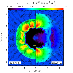
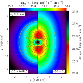
Figure 2: Left: Comparison of the net gain (neutrino heating minus cooling) in the nonrotating model s20.nr and in the rapidly-rotating model s20.$\pi$ as obtained with 2D angle-dependent transport at $160\,\mathrm{ms}$ after bounce. Due to its rapid rotation, model s20.$\pi$ has a larger shock radius, enhanced heating near the axis, but due to a positive specific angular momentum gradient in the postshock region at low latitudes, also much less convective overturn. Right: Comparison of the $\nu_{e}$ fluxes at $\epsilon_{\nu}=9.7\,\mathrm{MeV}$ in model s20.$\pi$ at $160\,\mathrm{ms}$ after bounce and as obtained with MGFLD (left section) and $S_{n}$ (right section). The radiation fields are oblate in the PNS core and deform to a prolate shape further out. Note that $S_{n}$ predicts a prolateness of the radiation field to much greater radii than MGFLD. The latter leads to nearly spherically symmetric radiation fields at radii greater than $\gtrsim\,$150–200 km. This result is largely independent of neutrino species and $\epsilon_{\nu}$.

In the left panel of Fig. 2 we plot the specific net gain, defined as neutrino heating $Q_{\nu}^{+}$ minus neutrino cooling $Q_{\nu}^{-}$ and contrast the $S_{n}$ results for the nonrotating model s20.nr (left half) with the rapidly rotating model s20.$\pi$ (right half) at $160\,\mathrm{ms}$ after bounce. In addition, we superpose velocity vectors to visualize the flow of matter. The qualitative and quantitative differences between the two models are large. In model s20.nr, there is strong neutrino heating in the immediate postshock region which drives strong convection. One also notes a slight deformation of the shock away from spherical symmetry which is indicative of the onset of the SASI. In model s20.$\pi$, on the other hand, the neutrino heating occurs very asymmetrically and primarily in polar regions where the neutrino flux is highest (see also the discussion in [37, 38, 21]). The shock is more extended along the poles, but there is a pronounced equatorial bulge with very little net heating. Convective overturn is confined to polar regions due to (1) a large positive specific angular momentum gradient at low latitudes, and (2) the absence of strong neutrino heating in these regions [39, 37, 40]. In addition, no signs of the SASI are apparent and the subsequent evolution of model s20.$\pi$ suggests that rapid rotation delays and modifies the SASI in axisymmetry. The situation may be different in 3D (e.g., [41, 42]).

The right panel of Fig. 2 visualizes the spectral flux density of $\nu_{e}$ at $\epsilon_{\nu}=9.7\,\mathrm{MeV}$ and at $160\,\mathrm{ms}$ after bounce in the rapidly spinning model s20.$\pi$ and contrasts the MGFLD result (left half) with that obtained with $S_{n}$ (right half). In both variants, the radiation field is oblate inside the PNS core, but quickly transitions to a prolate shape further out. The density gradient in the polar regions of the core is much steeper, allowing for much smaller neutrino sphere radii ($R_{\nu}=R(\tau\approx 2/3)$) and resulting in a dramatic enhancement of the polar neutrino flux [37, 38, 21]. The MGFLD result captures the overall systematics, but due to the diffusive nature of the 2D MGFLD approach, the radiation field asymmetry is smoothed out at low $\tau$ and becomes nearly spherical at radii $\gtrsim 150\,\mathrm{km}$. The angle-dependent variant, on the other hand, captures the true radiation-field asymmetry even at large radii. In the case of model s20.$\pi$, this results in polar neutrino heating that is locally larger by up to a factor of two than in the MGFLD calculation. The radiation field asymmetry in the nonrotating model s20.nr is much smaller and the radiation fields predicted by MGFLD and $S_{n}$ are more similar, while the $S_{n}$ calculation still yields locally $\sim 10\%$ greater heating rates.

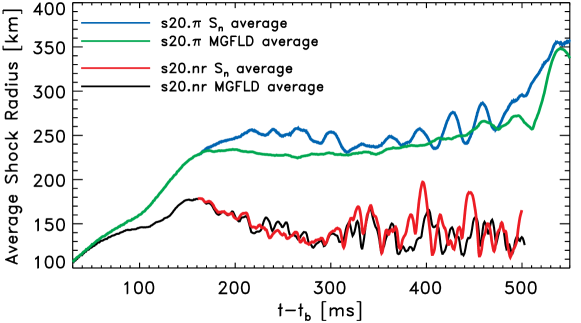
Figure 3: Average shock radius as a function of time after core bounce in MGFLD and $S_{n}$ variants of models s20.nr and s20.$\pi$. The large oscillations seen in the curves of the nonrotating model s20.nr are due to strong SASI oscillations and are somewhat more pronounced in the $S_{n}$ variant. The average shock radius of the rapidly rotating s20.$\pi$ settles at larger values than in the nonrotating case, but the growth of the SASI is slowed down by rapid rotation and only the $S_{n}$ model with its enhanced polar heating exhibits long-period SASI oscillations at intermediate postbounce times. See text and [21] for discussion.

Figure 3 visualizes the dynamical effect of angle-dependent neutrino transport on the postshock evolution of CCSNe by comparing the time evolution of the angle-averaged shock radii of the MGFLD and $S_{n}$ variants of models s20.nr and s20.$\pi$. In the latter, switching to $S_{n}$ leads to a shock expansion primarily in the polar regions where the increase in neutrino heating is greatest. However, increased neutrino cooling from the now also extended cooling region counteracts the shock expansion and lets it settle at a new, somewhat higher average radius. The larger radius and the increased local heating lead to an earlier onset of the rotationally-modified SASI in the $S_{n}$ variant. This is reflected in the earlier and more pronounced oscillations of the average shock radius. However, towards the end of the postbounce time covered by the simulations, the MGFLD variant’s average shock radius catches up and there is no large overall difference between the dynamics seen in the $S_{n}$ and MGFLD calculations of model s20.$\pi$.

The dynamical evolutions in the $S_{n}$ and MGFLD variants of the nonrotating model s20.nr are even more similar and the SASI shock excursions in the two variants remain practically in phase for almost $200\,\mathrm{ms}$. The $S_{n}$ calculation exhibits larger SASI excursions at later times, but, as in the case of model s20.$\pi$, there is no qualitative change between the MGFLD and $S_{n}$ postbounce evolutions despite stronger neutrino heating (by up to $30\%$ of the total heating rate at late times) in the latter.

2.3 Discussion

Neutrinos carry away $\sim 99\%$ of the gravitational energy of a neutron star formed in stellar collapse. Their transport and their interactions with matter are a central aspect of any CCSN model. Here, we have presented and summarized results from our recent VULCAN/2D simulations [21] that for the first time addressed for a multi-D simulation the long-term dependence of the postbounce dynamics of CCSNe on the neutrino transport technique employed. Comparing MGFLD and angle-dependent $S_{n}$ transport, we find that the former has difficulties in capturing physical radiation field asymmetries and preserving them at low optical depth. The $S_{n}$ approach self-consistently evolves the radiation field from the diffusion limit and isotropy to the free-streaming limit and forward-peakedness. $S_{n}$ generally leads to locally stronger neutrino heating, but the feedback in the supernova engine is sufficiently strong to lead to an adjustment of the system to a new equilibrium configuration without a true qualitative change when compared with MGFLD. Thus, it appears unlikely that differences in neutrino transport and/or interactions that result in by $10\%-30\%$ increased heating (as seen in our simulations) can have a strong impact on the CCSN dynamics. Larger effects seem necessary to turn the CCSN dud into an explosion.

The work of the Garching group [43, 5] and of the ORNL/FAU group [7] suggest that the inclusion of a general-relativistic monopole term in the otherwise Newtonian potential in combination with a soft EOS can increase the neutrino heating efficiency due to hardened neutrino spectra and may lead to explosion. Furthermore, [6] have shown in a simplified model with parametrized neutrino heating and cooling that explosions are more easily obtained in 2D than in 1D. This result may very well extend to 3D and supports and strengthens the CCSN community’s motivation to move towards 3D simulations.

3 A New, Fully General-Relativistic Approach in 3D

Today’s technically most advanced and physically most complete stellar collapse and long-term postbounce CCSN simulations are carried out in axisymmetry (2D), use angle-dependent neutrino transport or MGFLD either in full 2D [21, 12, 11, 44] or in a ray-by-ray approximation [43, 5, 45, 7] and implement Newtonian (magneto)hydrodynamics and gravity either in purely Newtonian fashion [21, 12, 11, 44] or with a GR monopole term in an otherwise Newtonian gravitational potential [43, 5, 45, 7]. The current state-of-the-art for axisymmetric GR core-collapse calculations, which traditionally have focussed on estimates of the GW signal from rotating core collapse and bounce, is set by [46] who performed conformally-flat calculations of the collapse and early postbounce phase with a finite-temperature ($T$) microphysical EOS and a simple deleptonization scheme [51] for the collapse phase in lieu of neutrino transport.

Current published 3D simulations do not yet rival their 2D counterparts in accuracy and physical completeness. Iwakami et al. [52, 42] investigated the SASI in 3D with steady-state initial conditions, spherical Newtonian gravity, a finite-$T$ microphysical EOS, parametrized neutrino heating/cooling, a cut-out core, and a fixed high accretion rate at the outer boundary. The Basel group [53], focussing on the GW signal of stellar collapse, performed 3D calculations of the collapse phase with a finite-$T$ microphysical EOS and the deleptonization scheme of [51] during collapse, but neglected neutrino transport and heating/cooling in the postbounce phase.

More physically accurate simulations with better neutrino physics and transport in the postbounce phase are required to address the explosion mechanism. Several groups are in the process of implementing codes with the necessary features (e.g., [45, 7, 54]).

In the following, we present our approach to 3D CCSN modeling which builds upon the tremendous recent progress in numerical relativity (see, e.g., [55]) and implements GR hydrodynamics and full GR curvature evolution in a variant of the Arnowitt-Deser-Misner (ADM) [56] $3+1$ formalism. This allows us to not only more accurately follow the CCSN hydrodynamics, but provides for the capability to form black holes dynamically and in 3D in failing core-collapse supernovae – something that is impossible in Newtonian or pseudo-GR formulations. Our approach makes heavy use of the Cactus computational toolkit [19] and is optimized for execution on supercomputers, implementing AMR, domain decomposition, parallel I/O, and hybrid MPI/OpenMP parallelism for improved scaling on massively-parallel systems.

In Section 3.1, we introduce our GR curvature and hydrodynamics formulation and discuss the computational infrastructure and the various physics components of our approach, and highlight parallel scaling results. In Section 3.2, we go on to discuss results obtained with our approach by [57, 48, 49] in the first set of GR simulations of rotating core collapse in 3D.

3.1 Computational Approach, Application Codes and Parallel Performance

We employ the open source software framework Cactus [58, 19] designed for computational scientific and engineering problems. It has a modular structure and enables scalable parallel computation across different architectures, as well as collaborative code development between different research groups.

Cactus consists of a central part, called the flesh, that provides core routines, and of components, called thorns. The flesh is independent of all thorns and provides the main program, which parses input parameters and activates the appropriate thorns, passing control to thorns as required. By itself, the flesh does very little science; to do any computational task the user must compile in thorns and activate them at run time. Parallelism, communication, load balancing, memory management, and I/O are handled by a special component, the driver, which is not part of the flesh and which can be transparently exchanged. The flesh (and the driver) have complete knowledge about the state of the application, allowing inspection and introspection through generic APIs.

Cactus runs on all current mainstream architectures. Applications, developed on standard workstations or laptops, can be seamlessly run on clusters or supercomputers. Cactus provides easy access to many cutting-edge software technologies being developed in the academic research community, including the Globus Metacomputing Toolkit [59, 60], HDF5 [61] parallel file I/O, the PETSc scientific library [62], AMR, multi-block methods [63], web interfaces [64], and advanced visualization tools (e.g. VisIt [65]).

The Einstein Toolkit [66] is a set of Cactus thorns providing infrastructure and basic functionality for GR applications codes using the variables of the ADM formalism [56]. Within a simulation, the ADM variables are employed for coupling GR curvature evolution with matter and radiation variables and also serve in run-time analysis of the simulation results, such as e.g. evaluating constraints, locating apparent horizons [67, 68] or event horizons [69], or calculating gravitational wave signals.

3.1.1 GR Curvature Evolution.

The Einstein equations are necessary for the correct description of gravity in the strong-field regime. They are a set of ten coupled, non-linear wave-type partial differential equations. We solve these equations using the BSSN formulation (e.g., [70] and references therein). This formulation, similar to ADM, breaks up the four-dimensional spacetime into $3+1$ dimensions, three spatial and one time dimensions. This leads to $25$ hyperbolic time evolution equations coupled to $9$ elliptic constraint equations.

Of the $25$ evolution equations, $8$ are not specified by the Einstein equations, but instead have to be chosen as gauge conditions to determine the time evolution of the curvilinear coordinates of spacetime. We choose the so-called $1+\log$ slicing condition and the $\Gamma$-driver shift condition [71, 57], which are standard gauge conditions used BSSN. They ensure stable, long-term time evolutions. The $9$ constraint equations have to be satisfied initially, requiring solving an elliptic system for setting up initial data, and remain then satisfied under time evolution up to within the discretization error. We monitor the constraints during time evolution and do not re-solve them. The resulting equations for the BSSN system and the gauge conditions can be time-evolved with standard discretization methods.

We are using the Kranc package [72, 73] for automatic code generation for the BSSN formulation, gauge conditions, and constraint equations. Kranc is a Mathematica package which generates Cactus thorns from equations. Starting from equations in Mathematica format which specify a system of PDEs in abstract index notation, Kranc discretizes the equations and generates a complete Cactus thorn that evaluates these equations. Kranc-generated thorns use all relevant Cactus APIs for initial data setup, analysis, time integration, and AMR.

Automatic code generation greatly reduces the time and effort necessary to implement the BSSN equations, since these contain about 5,000 individual terms. Kranc also allows us to experiment with modifications to the formulation, e.g. to increase accuracy near singularities, and with modifications to low-level implementation details (loop blocking, vectorization) to achieve higher efficiencies on modern computer architectures.

We have implemented the BSSN equations in an open-source Cactus thorn arrangement called McLachlan [75, 74] in the XiRel [77, 76] project. McLachlan is a full-featured BSSN solver able to simulate not only stellar collapse, but also relativistic binary systems of black holes or neutron stars [75].

3.1.2 GR Hydrodynamics, Microphysics and Neutrinos

On the GR hydrodynamics (GRHD) side, we implement the Valencia formalism of GRHD [78, 79] which is based on a dimensionally-split flux-conservative high-resolution shock-capturing finite-volume approach. These methods are generally of lower order than those used for the spacetime curvature evolution, i.e., second-order in space and second-order in time. The main reason for this is not only that the discretization of the GR hydrodynamics problem becomes much more complicated with increasing order, but also that all higher-order methods must drop back to first order near discontinuities in the flow in order to prevent spurious oscillations in the solution. GR magnetohydrodynamics (GRMHD) is an extension to GRHD and can be straightforwardly implemented within the same general formalism [80, 81].

The Zelmani CCSN package proper is a collection of Cactus thorns implementing GRHD, a finite-temperature nuclear EOS, neutrino leakage, and heating [57, 48, 49, 82]. We generally use the name Zelmani synonymously to refer to the entire set of codes involved in our 3D GR CCSNe simulations, including McLachlan, Carpet, CactusEinstein, and Cactus. The GRHD module is based on a modified version of the open-source Whisky code [83, 84] that allows for general, finite-temperature EOS and neutrino-matter interactions. In our simulations, we employ PPM reconstruction of variables at cell interfaces and the approximate HLLE solver [85] for the relativistic Riemann problem.

Fully relativistic neutrino radiation transport is a formidable problem. Multi-D GR formulations exist (e.g., [86, 87]), but are still awaiting their first implementations. While we are actively exploring various ways to implement GR transport, we presently resort to the deleptonization scheme of [51] for collapse and employ neutrino leakage (e.g., [88]) and parametrized heating in the postbounce phase [82, 6]. Neutrino pressure contributions are included via the approximation discussed in [51].

3.1.3 Adaptive Mesh Refinement and Parallel Scaling.

Carpet [89, 63, 90] is our AMR driver for the Cactus framework. Carpet acts as a driver layer for Cactus, providing adaptive mesh refinement, multi-patch capability, and efficient parallelization and I/O. We make both Cactus and Carpet publicly available as open source, and both are also used by a number of other numerical relativity and computational astrophysics groups.

Carpet provides spatial discretization based on highly efficient block-structured, decomposed, logically Cartesian grids with hybrid MPI/OpenMP [91, 92] parallelism. Carpet offers both AMR and multi-block capabilities, covering the domain with sets of distorted, logically rectangular blocks of grids. Time integration is performed via the recursive Berger–Oliger AMR scheme [93], including subcycling in time. As demonstrated in the left panel of Fig. 4, Carpet presently scales well to more than 16,000 cores with AMR on Leadership HPC systems.

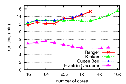
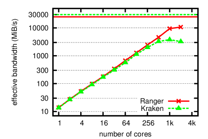
Figure 4: Left: Weak scaling benchmark for spacetime curvature and GRHD evolution of a single neutron star (Ranger, Kraken, Queen Bee) or of a single black hole (Franklin) with nine levels of mesh refinement. Ideal scaling would be an horizontal line in both cases. Cactus/Carpet scales well up to more than 16,000 cores. Ranger and Kraken are the currently largest machines on the NSF TeraGrid, Queen Bee is the largest machine on LONI and Franklin is a large DoE/NERSC system. Right: Cumulative I/O bandwidth for writing checkpoint files in parallel. This measurement includes application overhead. The theoretical peak bandwidth is shown as an horizontal line. Cactus/Carpet is able to achieve a significant fraction of this.

Carpet employs HDF5 [61] for parallel, binary I/O, which is also used for checkpointing and restarting. The right panel of Fig. 4 depicts results of I/O benchmarks, comparing the achieved I/O bandwidth to the theoretical peak bandwidth on selected HPC systems. Carpet achieves a significant fraction of this already on about 1,000 cores.

Although the speed and performance of high-end computers have increased dramatically over the last decade, the ease of programming such parallel computers has not progressed. To address these issues in computational modeling in general and in numerical relativity and CCSN simulations in particular, we are developing the Alpaca tools [95, 94]. In contrast to existing debuggers and profilers, these tools work at the much higher level of the physical equations and their discretizations and not at the level of individual lines of code or variables. The Alpaca tools are not external to the application, but are built-in, so that they have direct high-level access to information about the running application, and can interact with the user on a correspondingly high level.

3.2 Computational Costs, Simulations and First Results

A typical simulation setup to track collapse and postbounce CCSN evolution with GR curvature evolution and GRHD uses a 9-level AMR grid hierarchy with $\sim 400^{3}$ computational zones each, providing high resolution near the center ($\delta x\lesssim 300\,\mathrm{m}$), while encompassing the inner $\sim 5000\,\mathrm{km}$ of the dying star. There are about $400$ 3D grid functions required for curvature and GRHD which translates to a memory footprint of $\sim 2\,\mathrm{TB}$ (including inter-process buffers assuming 1024 processes). A single point update requires $\sim 50\,\mathrm{kflop}$ and $\sim 1\,\mathrm{million}$ fine grid updates are required, resulting in a total cost of $\sim 1500\,\mathrm{Pflop}$ for a single simulation. On 1024 compute cores and assuming a sustained performance of $1\,\mathrm{Gflop/s}$ per core, such a simulation requires $\sim 17\,\mathrm{days}$ to complete. If radiation transport, even in approximate ray-by-ray fashion, is included, the memory footprint and the total number of required flops must be scaled by a factor of $10-100$.

As a first application of our Cactus-based 3D GR Zelmani CCSN code, we are considering the collapse and very early postbounce phase of rapidly rotating iron cores with an emphasis on the study of rotational multi-D dynamics leading to the emission of gravitational waves (GWs). The latter may, in combination with neutrinos, play an important future role as diagnostic tools for the CCSN mechanism [96, 3] and in the case of rotating collapse can provide information on the nuclear EOS, as well as on the rotation rate of the inner core at bounce [46].

We have carried out the first parameter study of rotating core collapse in 3D GR, investigating the dependence of dynamics and GW signal on progenitor stellar structure and precollapse rotational setup, specified by the degree of differential rotation and the initial central angular velocity. Since these simulations were run with an earlier version of Zelmani, postbounce deleptonization was neglected. The results of this study were extensively discussed in [57, 48, 49] and we highlight a number of the findings in the following.

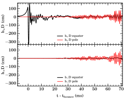
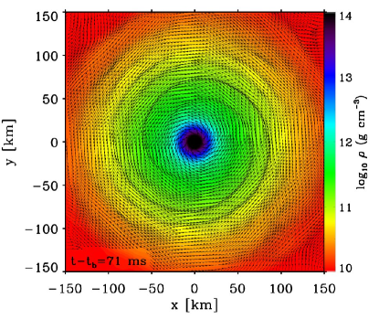
Figure 5: Left: Gravitational wave (GW) signals of the $+$ polarization (top, $h_{+}\,D$, where $D$ is the source distance) and of the $\times$ polarization (bottom, $h_{\times}D$), emitted by model E20 as a function of postbounce time and as seen by polar (red lines) and equatorial (black lines) observers. Collapse and bounce are axisymmetric (only $h_{+}$ and emission only away from the symmetry axis) while at postbounce times nonaxisymmetric dynamics and GW emission develop. Right: Density colormap showing the inner $150$x$150$ km of the equatorial plane ($z=0$) at $71\,\mathrm{ms}$ after bounce in the 3D GR model E20A. Velocity vectors are superposed and mark spiral density waves that develop due to a nonaxisymmetric instability in the PNS and propagate through the postshock region.

In the left panel of Fig. 5 we plot the two GW polarizations $h_{+}$ and $h_{\times}$, both scaled by distance $D$ to the source and in units of centimeters, as extracted from the multi-D dynamics in our model E20A that is based on the rotating $20$-$M_{\odot}$ progenitor star of [97]. Its precollapse central angular velocity is $\sim 3.1\,\mathrm{rad\,s}^{-1}$ and its precollapse rotation rate $\beta=T/|W|$ is $\sim 0.004$. The corresponding values early after bounce are $\sim 4\,\mathrm{rad\,ms}^{-1}$ and $\sim 0.09$. The simulation is run in 3D from the onset of collapse to $\sim 70\,\mathrm{ms}$ after bounce.

We find that model E20A, like all other considered models, stays axisymmetric through collapse, core bounce, and the early postbounce phase. At bounce, the large deceleration of the inner core’s infall leads to a large negative spike in the waveform clearly visible in $h_{+}D$ as seen by an equatorial observer and shown in the left panel of Fig. 5. Due to the axisymmetry of the rotating collapse dynamics, GWs are emitted only in one polarization (linear polarization; here, due to the choice of source orientation, in the $+$ polarization) and only away from the symmetry axis of the system. After bounce and on a timescale of $\gtrsim 20-40\,\mathrm{ms}$ nonaxisymmetric dynamics develops in the PNS and is likely due to a corotation-type instability in which an azimuthal mode picks up power from the axisymmetric background rotation at the point where its mode pattern speed is in corotation with the fluid (see, e.g., [98]). The quadrupole components ($\ell=2,m=2$) of the nonaxisymmetric dynamics are reflected in the late-time GW signal as a quasi-periodic, elliptically polarized signal, strongly correlated in $h_{+}$ and $h_{\times}$ and emitted at twice the $m=2$ pattern speed. This nonaxisymmetric GW emission is smaller in amplitude than the burst associated with core bounce, but, due to its longer duration, the total energy emission is greater and the emission’s narrowband nature favors detection by GW observatories such as LIGO [99, 96].

Corotation instabilities are well known from studies of astrophysical disks and belong to a class of dynamical shear instabilities that draw from the shear energy stored in differential rotation and transport angular momentum outward in spiral waves. Differential rotation is abundant in the postshock region [57, 40] and the spiral waves are apparent in the right panel of Fig. 5 that depicts the density distribution with superposed fluid velocity vectors in the equatorial plane of model E20A at $\sim 70\,\mathrm{ms}$ after bounce.

4 Summary and Outlook

The challenging complexity and non-linearity of the CCSN problem and current technical and computational limitations call for a broad computational program with multiple modeling approaches. In this contribution to SciDAC 2009, we introduced two CCSN simulation programs and discussed their recent results. The first, VULCAN/2D, a full CCSN code with an implementation of the angle-dependent and MGFLD radiation-MHD equations, is capable of studying all presently discussed CCSN mechanisms, but is limited to axisymmetry and Newtonian gravity and dynamics. Being based on proven legacy technology and despite not employing the massively-parallel domain-decomposition paradigm, VULCAN/2D runs very efficiently on a modest number of compute cores and yields a high science output per flop (e.g., [23, 22, 37, 12, 13, 11, 25, 26, 21]). This includes the first long-term true multi-D angle-dependent neutrino transport CCSN calculations highlighted in this article. The result of this study is an example of Mazurek’s law. Applied to the present situation, it states that in the tightly-coupled CCSN phenomenon, even a rather significant ($\gtrsim 10\%-30\%$) change of the postbounce conditions, in this case, of the neutrino heating rate, is absorbed by the strong feedback between radiation, hydrodynamics, EOS, and gravity and no qualitative change results.

The frontier of CCSN modeling is clearly 3D and the hope is that the additional degree of freedom and the more accurate representation of (turbulent) convection and SASI help produce successful and powerful explosions whose asymptotic energies match observations. We approach the computationally and technically challenging step to 3D with the code Zelmani that is based on the open-source Cactus framework and uses scalable AMR via the Carpet driver module that implements state-of-the-art HPC paradigms, including hybrid MPI/OpenMP parallelism for modern massively-parallel multi-core architectures. Zelmani is set apart from other 3D codes (e.g., [53, 45, 7]) by its full GR nature, evolving Einstein’s equations from one spatial $3$-hypersurface to the next and treating the dynamics fully relativistically instead of re-solving a Newtonian or pseudo-relativistic Poisson equation at every timestep coupled to Newtonian hydrodynamics. Dynamical spacetime evolution not only enables us to study the impact of GR on the CCSN evolution, but also allows us to investigate the dynamical formation of black holes in failing core-collapse supernovae. Such collapsars are considered as likely candidates for the central engines of gamma-ray bursts (GRBs; e.g., [1]), but their dynamical formation has not been modeled and remains to be understood.

While still under development towards a full GR radiation-MHD CCSN code, Zelmani has already been applied to 3D GR hydrodynamic studies of rotating stellar collapse, leading to an improved understanding of the gravitational wave signature of CCSNe [57, 49, 48]. In its completed form, Zelmani will allow us to take full advantage of petaflop supercomputers to comprehensively address the CCSN problem and the CCSN-GRB relationship.

It is a pleasure to acknowledge help from and stimulating conversations with J. Murphy, L. Dessart, E. Abdikamalov, G. Allen, D. Arnett, W. Benger, S. Bruenn, P. Diener, H. Dimmelmeier, I. Hawke, I. Hinder, K. Kotake, C. Meakin, B. Messer, A. Mezzacappa, J. Nordhaus, L. Rezzolla, B. Schutz, E. Seidel, S. Su, J. Tohline, and S. Woosley. The Cactus-based part of this work would not have been possible without the invaluable help of our late colleague Thomas Radke whom we miss dearly both personally and professionally. CDO is supported by a Sherman Fairchild Prize Fellowship at Caltech and by an Otto Hahn Prize of the Max Planck Society. AB is partially supported by the Scientific Discovery through Advanced Computing (SciDAC) program of the US Department of Energy under grant number DE-FC02-06ER41452. EO is supported by a Natural Sciences and Engineering Research Council of Canada postgraduate scholarship. The development of Cactus, the Einstein Toolkit, and the performance tools is supported by the NSF grants XiRel (no. 0701566), Alpaca (no. 0721915), and Blue Waters (no. 0725070). Simulations and benchmarks were performed on Queen Bee at LONI under allocation loni_numrel03, and on Kraken at NICS and Ranger at TACC under the NSF TeraGrid allocation TG-MCA02N014. Additional computations were performed at the National Energy Research Scientific Computing Center (NERSC), which is supported by the Office of Science of the US Department of Energy under contract DE-AC03-76SF00098.

References

- [1] Woosley S E and Bloom J S 2006 Ann. Rev. Astron. Astrophys. 44 507
- [2] Heger A, Fryer C L, Woosley S E, Langer N and Hartmann D H 2003 Astrophys. J. 591 288
- [3] Ott C D 2009 Submitted to Class. Quant. Grav. arXiv:0905.2797 [astro-ph]
- [4] Janka H T, Langanke K, Marek A, Martínez-Pinedo G and Müller B 2007 Phys. Rep. 442 38
- [5] Marek A and Janka H T 2009 Astrophys. J. 694 664
- [6] Murphy J W and Burrows A 2008 Astrophys. J. 688 1159
- [7] Bruenn S W, Mezzacappa A, Hix W R, Blondin J M, Marronetti P, Messer O E B, Dirk C J and Yoshida S 2009 AIP Phys. Conf. Ser. (AIP Phys. Conf. Ser. vol 1111) ed Giobbi G, Tornambe A, Raimondo G, Limongi M, Antonelli L A, Menci N and Brocato E p 593
- [8] Scheck L, Janka H T, Foglizzo T and Kifonidis K 2008 Astron. Astrophys. 477 931
- [9] LeBlanc J M and Wilson J R 1970 Astrophys. J. 161 541
- [10] Bisnovatyi-Kogan G S, Popov I P and Samokhin A A 1976 Astrophys. Space Sci. 41 287
- [11] Burrows A, Dessart L, Livne E, Ott C D and Murphy J 2007 Astrophys. J. 664 416
- [12] Burrows A, Livne E, Dessart L, Ott C D and Murphy J 2006 Astrophys. J. 640 878
- [13] Burrows A, Livne E, Dessart L, Ott C D and Murphy J 2007 Astrophys. J. 655 416
- [14] Ott C D, Burrows A, Dessart L and Livne E 2006 Phys. Rev. Lett. 96 201102
- [15] Weinberg N N and Quataert E 2008 Mon. Not. Roy. Astron. Soc. 387 L64
- [16] Cerdá-Durán P, Font J A and Dimmelmeier H 2007 Astron. Astrophys. 474 169
- [17] Rosswog S 2009 Preprint, ArXiv:0903.5075 [astro-ph]
- [18] Thorne K S 1987 300 Years of Gravitation ed Hawking S W and W I (Cambridge, UK: Cambridge University Press)
- [19] Cactus Computational Toolkit home page URL http://www.cactuscode.org/
- [20] Livne E 1993 Astrophys. J. 412 634
- [21] Ott C D, Burrows A, Dessart L and Livne E 2008 Astrophys. J. 685 1069
- [22] Livne E, Burrows A, Walder R, Lichtenstadt I and Thompson T A 2004 Astrophys. J. 609 277
- [23] Ott C D, Burrows A, Livne E and Walder R 2004 Astrophys. J. 600 834
- [24] Livne E, Dessart L, Burrows A and Meakin C A 2007 Astrophys. J. Supp. Ser. 170 187
- [25] Dessart L, Burrows A, Livne E and Ott C D 2006 Astrophys. J. 645 534
- [26] Dessart L, Burrows A, Ott C D, Livne E, Yoon S Y and Langer N 2006 Astrophys. J. 644 1063
- [27] Dessart L, Burrows A, Livne E and Ott C D 2008 Astrophys. J. Lett. 673 L43
- [28] Shen H, Toki H, Oyamatsu K and Sumiyoshi K 1998 Nucl. Phys. A 637 435
- [29] Bruenn S W 1985 Astrophys. J. Supp. Ser. 58 771
- [30] Castor J I 2004 Radiation Hydrodynamics (Radiation Hydrodynamics, by John I. Castor, pp. 368. ISBN 0521833094. Cambridge, UK: Cambridge University Press, November 2004.)
- [31] Burrows A, Reddy S and Thompson T A 2006 Nuclear Physics A 777 356
- [32] Thompson T A, Burrows A and Horvath J E 2000 Phys. Rev. C. 62 035802
- [33] Hubeny I and Burrows A 2007 Astrophys. J. 659 1458
- [34] Woosley S E, Heger A and Weaver T A 2002 Rev. Mod. Phys. 74 1015
- [35] Messer O E B, Mezzacappa A, Bruenn S W and Guidry M W 1998 Astrophys. J. 507 353
- [36] Thompson T A, Burrows A and Pinto P A 2003 Astrophys. J. 592 434
- [37] Walder R, Burrows A, Ott C D, Livne E, Lichtenstadt I and Jarrah M 2005 Astrophys. J. 626 317
- [38] Kotake K, Yamada S and Sato K 2003 Astrophys. J. 595 304
- [39] Fryer C L and Heger A 2000 Astrophys. J. 541 1033
- [40] Ott C D, Burrows A, Thompson T A, Livne E and Walder R 2006 Astrophys. J. Suppl. Ser. 164 130
- [41] Yamasaki T and Foglizzo T 2008 Astrophys. J. 679 607
- [42] Iwakami W, Kotake K, Ohnishi N, Yamada S and Sawada K 2008 submitted to ApJ, arXiv:0811.0651 [astro-ph]
- [43] Buras R, Janka H T, Rampp M and Kifonidis K 2006 Astron. Astrophys. 457 281
- [44] Swesty F D and Myra E S 2009 Astrophys. J. Supp. Ser. 181 1
- [45] Bruenn S W, Dirk C J, Mezzacappa A, Hayes J C, Blondin J M, Hix W R and Messer O E B 2006 J. Phys. Conf. Ser. 46 393
- [46] Dimmelmeier H, Ott C D, Marek A and Janka H T 2008 Phys. Rev. D. 78 064056
- [47] Isenberg J A 2008 International Journal of Modern Physics D 17 265
- [48] Ott C D, Dimmelmeier H, Marek A, Janka H T, Hawke I, Zink B and Schnetter E 2007 Phys. Rev. Lett. 98 261101
- [49] Ott C D, Dimmelmeier H, Marek A, Janka H T, Zink B, Hawke I and Schnetter E 2007 Class. Quant. Grav. 24 139
- [50] Cerdá-Durán P, Faye G, Dimmelmeier H, Font J A, Ibáñez J M, Müller E and Schäfer G 2005 Astron. Astrophys. 439 1033
- [51] Liebendörfer M 2005 Astrophys. J. 633 1042
- [52] Iwakami W, Kotake K, Ohnishi N, Yamada S and Sawada K 2008 Astrophys. J. 678 1207
- [53] Scheidegger S, Fischer T, Whitehouse S C and Liebendörfer M 2008 Astron. Astrophys. 490 231
- [54] Liebendörfer M, Whitehouse S C and Fischer T 2009 Astrophys. J. 698 1174
- [55] Pretorius F 2007 Lecture Notes to appear in the book: ”Relativistic Objects in Compact Binaries: From Birth to Coalescence,” arxiv:0710.1338 [gr-qc]
- [56] Arnowitt R, Deser S and Misner C W 1962 Gravitation: An introduction to current research ed Witten L (New York: John Wiley) pp 227–265 (Preprint gr-qc/0405109)
- [57] Ott C D 2006 Stellar Iron Core Collapse in 3+1 General Relativity and The Gravitational Wave Signature of Core-Collapse Supernovae Ph.D. thesis Universität Potsdam Potsdam, Germany URL http://nbn-resolving.de/urn/resolver.pl?urn=urn:nbn:de:kobv:5%17-opus-12986
- [58] Goodale T, Allen G, Lanfermann G, Massó J, Radke T, Seidel E and Shalf J 2003 Vector and Parallel Processing – VECPAR’2002, 5th International Conference, Lecture Notes in Computer Science (Berlin: Springer)
- [59] Allen G, Dramlitsch T, Foster I, Goodale T, Karonis N, Ripeanu M and Toonen B 2000 Proceedings of 4th Globus Retreat, July 30 to August 1 2000, Pittsburg URL http://citeseer.nj.nec.com/article/allen00cactusg.html
- [60] Globus Project Home Page URL http://www.globus.org
- [61] HDF 5: Hierarchical Data Format Version 5 URL http://hdf.ncsa.uiuc.edu/HDF5/
- [62] Balay S, Buschelman K, Gropp W D, Kaushik D, Knepley M, McInnes L C, Smith B F and Zhang H 2001 PETSc home page http://www.mcs.anl.gov/petsc URL http://www.mcs.anl.gov/petsc
- [63] Schnetter E, Diener P, Dorband N and Tiglio M 2006 Class. Quantum Grav. 23 S553–S578
- [64] Cactus web server (live demonstration) URL http://cactus.cct.lsu.edu:5555/
- [65] VisIt Visualization Tool URL https://wci.llnl.gov/codes/visit/
- [66] Schnetter E 2008 Multi-physics coupling of Einstein and hydrodynamics evolution: A case study of the Einstein Toolkit cBHPC 2008 (Component-Based High Performance Computing)
- [67] Thornburg J 1996 Phys. Rev. D 54 4899–4918
- [68] Thornburg J 2004 Class. Quantum Grav. 21 743–766
- [69] Diener P 2003 Class. Quantum Grav. 20 4901–4917
- [70] Alcubierre M, Brügmann B, Dramlitsch T, Font J A, Papadopoulos P, Seidel E, Stergioulas N and Takahashi R 2000 Phys. Rev. D 62 044034
- [71] Alcubierre M, Brügmann B, Diener P, Koppitz M, Pollney D, Seidel E and Takahashi R 2003 Phys. Rev. D 67 084023
- [72] Husa S, Hinder I and Lechner C 2006 Comput. Phys. Comm. 174 983–1004
- [73] Kranc: Automated Code Generation URL http://numrel.aei.mpg.de/Research/Kranc/
- [74] McLachlan, a Public BSSN Code URL http://www.cct.lsu.edu/~eschnett/McLachlan/index.html
- [75] Brown D, Diener P, Sarbach O, Schnetter E and Tiglio M 2009 Phys. Rev. D 79 044023
- [76] XiRel: Next Generation Infrastructure for Numerical Relativity URL http://www.cct.lsu.edu/xirel/
- [77] Tao J, Allen G, Hinder I, Schnetter E and Zlochower Y 2008 XiRel: Standard benchmarks for numerical relativity codes using Cactus and Carpet Tech. Rep. CCT-TR-2008-5 Louisiana State University URL http://www.cct.lsu.edu/CCT-TR/CCT-TR-2008-5
- [78] Banyuls F, Font J A, Ibáñez J M, Martí J M and Miralles J A 1997 Astrophys. J. 476 221
- [79] Font J A, Goodale T, Iyer S, Miller M, Rezzolla L, Seidel E, Stergioulas N, Suen W M and Tobias M 2002 Phys. Rev. D 65 084024
- [80] Cerdá-Durán P, Font J A, Antón L and Müller E 2008 Astron. Astrophys. 492 937
- [81] Giacomazzo B and Rezzolla L 2007 Class. Quantum Grav. 24 S235–S258
- [82] O’Connor E and Ott C D 2009 in preparation
- [83] Baiotti L, Hawke I, Montero P J, Löffler F, Rezzolla L, Stergioulas N, Font J A and Seidel E 2005 Phys. Rev. D 71 024035
- [84] Whisky, EU Network GR Hydrodynamics Code URL http://www.whiskycode.org/
- [85] Einfeldt B 1988 SIAM J. Numer. Anal. 25 294–318
- [86] Cardall C and Mezzacappa A 2003 Phys. Rev. D. 68 023006
- [87] Zink B 2008 arXiv:0810.5349 [astro-ph]
- [88] Ruffert M, Janka H T and Schaefer G 1996 Astron. Astrophys. 311 532–566
- [89] Schnetter E, Hawley S H and Hawke I 2004 Class. Quantum Grav. 21 1465–1488
- [90] Mesh refinement with Carpet URL http://www.carpetcode.org/
- [91] MPI: Message Passing Interface Forum URL http://www.mpi-forum.org/
- [92] OpenMP: Simple, Portable, Scalable SMP Programming URL http://www.openmp.org/
- [93] Berger M J and Oliger J 1984 J. Comput. Phys. 53 484–512
- [94] Alpaca: Tools for Application-Level Profiling and Correctness Analysis URL http://www.cct.lsu.edu/~eschnett/Alpaca/
- [95] Schnetter E, Allen G, Goodale T and Tyagi M 2008 Alpaca: Cactus tools for application level performance and correctness analysis Tech. Rep. CCT-TR-2008-2 Louisiana State University URL http://www.cct.lsu.edu/CCT-TR/CCT-TR-2008-2
- [96] Ott C D 2009 Class. Quant. Grav. 26 063001
- [97] Heger A, Langer N and Woosley S E 2000 Astrophys. J. 528 368
- [98] Watts A L, Andersson N and Jones D I 2005 Astrophys. J. Lett. 618 L37
- [99] LIGO URL http://ligo.caltech.edu
- [100] Lattimer J 2009 private communication
- [101] Burrows A 2001 private communication