On condition numbers of polynomial eigenvalue problems with nonsingular leading coefficients

Nikolaos Papathanasiou  and Panayiotis Psarrakos11footnotemark: 1 Department of Mathematics, National Technical University of Athens, Zografou Campus, 15780 Athens, Greece (nipapath@mail.ntua.gr, N. Papathanasiou; ppsarr@math.ntua.gr, P. Psarrakos).
Abstract

In this paper, we investigate condition numbers of eigenvalue problems of matrix polynomials with nonsingular leading coefficients, generalizing classical results of matrix perturbation theory. We provide a relation between the condition numbers of eigenvalues and the pseudospectral growth rate. We obtain that if a simple eigenvalue of a matrix polynomial is ill-conditioned in some respects, then it is close to be multiple, and we construct an upper bound for this distance (measured in the euclidean norm). We also derive a new expression for the condition number of a simple eigenvalue, which does not involve eigenvectors. Moreover, an Elsner-like perturbation bound for matrix polynomials is presented.

Dedicated to the memory of James H. Wilkinson (1919–1986)

Keywords: matrix polynomial, eigenvalue, perturbation, condition number, pseudospectrum.

AMS Subject Classifications: 15A18, 15A22, 65F15, 65F35.

1 Introduction

The notions of condition numbers of eigenproblems and eigenvalues quantify the sensitivity of eigenvalue problems [5, 7, 11, 12, 17, 19, 20, 21, 23, 24, 26, 27, 28]. They are widely appreciated tools for investigating the behavior under perturbations of matrix-based dynamical systems and of algorithms in numerical linear algebra. An eigenvalue problem is called ill-conditioned (resp., well-conditioned) if its condition number is sufficiently large (resp., sufficiently small).

In 1965, Wilkinson [26] introduced the condition number of a simple eigenvalue λ0subscript𝜆0{\lambda}_{0} of a matrix A𝐴A while discussing the sensitivity of λ0subscript𝜆0{\lambda}_{0} in terms of the associated right and left eigenspaces. Two years later, Smith [20] obtained explicit expressions for certain condition numbers related to the reduction of matrix A𝐴A to its Jordan canonical form. In early 1970’s, Stewart [21] and Wilkinson [27] used the condition number of the simple eigenvalue λ0subscript𝜆0{\lambda}_{0} to construct a lower bound and an upper bound for the distance from A𝐴A to the set of matrices that have λ0subscript𝜆0{\lambda}_{0} as a multiple eigenvalue, respectively. Recently, the notion of the condition number of simple eigenvalues of matrices has been extended to multiple eigenvalues of matrices [5, 11, 12] and to eigenvalues of matrix polynomials [12, 24].

In this article, we are concerned with conditioning for the eigenvalue problem of a matrix polynomial P(λ)𝑃𝜆P({\lambda}) with a nonsingular leading coefficient, generalizing known results of matrix perturbation theory [5, 8, 11, 20, 27]. In the next section, we give the definitions and the necessary background on matrix polynomials. In Section 3, we investigate the strong connection between the condition numbers of the eigenvalues of P(λ)𝑃𝜆P({\lambda}) and the growth rate of its pseudospectra. This connection allows us to portrait the abstraction of the condition numbers of eigenvalues. In Section 4, we examine the relation between the condition number of a simple eigenvalue λ0subscript𝜆0{\lambda}_{0} of P(λ)𝑃𝜆P({\lambda}) and the distance from P(λ)𝑃𝜆P({\lambda}) to the set of matrix polynomials that have λ0subscript𝜆0{\lambda}_{0} as a multiple eigenvalue. In particular, we see that if the condition number of λ0subscript𝜆0{\lambda}_{0} is sufficiently large, then this eigenvalue is close to be multiple. In Section 5, we provide a new expression for the condition number of a simple eigenvalue λ0subscript𝜆0{\lambda}_{0} of P(λ)𝑃𝜆P({\lambda}), which involves the distances from λ0subscript𝜆0{\lambda}_{0} to the rest of the eigenvalues of P(λ)𝑃𝜆P({\lambda}). Finally, in Section 6, we present an extension of the Elsner Theorem [8, 22, 23] to matrix polynomials. Simple numerical examples are also given to illustrate our results.

2 Preliminaries on matrix polynomials

Consider an n×n𝑛𝑛n\times n matrix polynomial

P(λ)=Amλm+Am1λm1++A1λ+A0,𝑃𝜆subscript𝐴𝑚superscript𝜆𝑚subscript𝐴𝑚1superscript𝜆𝑚1subscript𝐴1𝜆subscript𝐴0P({\lambda})\,=\,A_{m}{\lambda}^{m}+A_{m-1}{\lambda}^{m-1}+\cdots+A_{1}{\lambda}+A_{0}, (1)

where λ𝜆{\lambda} is a complex variable and Ajn×nsubscript𝐴𝑗superscript𝑛𝑛A_{j}\in\mathbb{C}^{n\times n} (j=0,1,,m𝑗01𝑚j=0,1,\dots,m) with detAm0subscript𝐴𝑚0\det A_{m}\neq 0. The study of matrix polynomials has a long history, especially with regard to their spectral analysis, which leads to the solutions of higher order linear systems of differential equations. The suggested references on matrix polynomials are [10, 14, 16].

A scalar λ0subscript𝜆0\,{\lambda}_{0}\in\mathbb{C}\, is called an eigenvalue of P(λ)𝑃𝜆P({\lambda}) if the system P(λ0)x=0𝑃subscript𝜆0𝑥0\,P({\lambda}_{0})x=0\, has a nonzero solution x0nsubscript𝑥0superscript𝑛\,x_{0}\in\mathbb{C}^{n}, known as a right eigenvector of P(λ)𝑃𝜆P({\lambda}) corresponding to λ0subscript𝜆0{\lambda}_{0}. A nonzero vector y0nsubscript𝑦0superscript𝑛y_{0}\in\mathbb{C}^{n} that satisfies y0P(λ0)=0superscriptsubscript𝑦0𝑃subscript𝜆00y_{0}^{*}P({\lambda}_{0})=0 is called a left eigenvector of P(λ)𝑃𝜆P({\lambda}) corresponding to λ0subscript𝜆0{\lambda}_{0}. The set of all eigenvalues of P(λ)𝑃𝜆P({\lambda}) is the spectrum of P(λ)𝑃𝜆P({\lambda}), σ(P)={λ:detP(λ)=0},𝜎𝑃conditional-set𝜆𝑃𝜆0\,\sigma(P)=\left\{{\lambda}\in\mathbb{C}:\det P({\lambda})=0\right\},\, and since detAm0,subscript𝐴𝑚0\,\det A_{m}\neq 0,\, it contains no more than nm𝑛𝑚nm distinct (finite) elements. The algebraic multiplicity of an eigenvalue λ0σ(P)subscript𝜆0𝜎𝑃\,{\lambda}_{0}\in\sigma(P)\, is the multiplicity of λ0subscript𝜆0{\lambda}_{0} as a zero of the (scalar) polynomial detP(λ)𝑃𝜆\det P({\lambda}), and it is always greater than or equal to the geometric multiplicity of λ0subscript𝜆0{\lambda}_{0}, that is, the dimension of the null space of matrix P(λ0)𝑃subscript𝜆0P({\lambda}_{0}).

2.1 Jordan structure and condition number of the eigenproblem

Let λ1,λ2,subscript𝜆1subscript𝜆2{\lambda}_{1},{\lambda}_{2}, ,λrσ(P)subscript𝜆𝑟𝜎𝑃\dots,{\lambda}_{r}\in{\sigma}(P) be the eigenvalues of P(λ)𝑃𝜆P({\lambda}), where each λisubscript𝜆𝑖{\lambda}_{i} appears exactly kisubscript𝑘𝑖k_{i} times if and only if its geometric multiplicity is kisubscript𝑘𝑖k_{i} (i=1,2,,r𝑖12𝑟i=1,2,\dots,r). Suppose also that for an eigenvalue λiσ(P)subscript𝜆𝑖𝜎𝑃{\lambda}_{i}\in{\sigma}(P), there exist xi,1,xi,2,,xi,sinsubscript𝑥𝑖1subscript𝑥𝑖2subscript𝑥𝑖subscript𝑠𝑖superscript𝑛\,x_{i,1},x_{i,2},\dots,x_{i,s_{i}}\in\mathbb{C}^{n}\, with xi,10,subscript𝑥𝑖10\,x_{i,1}\neq 0,\, such that

j=1ξ1(j1)!P(j1)(λi)xi,ξj+1= 0;ξ=1,2,,si,formulae-sequencesuperscriptsubscript𝑗1𝜉1𝑗1superscript𝑃𝑗1subscript𝜆𝑖subscript𝑥𝑖𝜉𝑗1 0𝜉12subscript𝑠𝑖\sum_{j=1}^{\xi}\frac{1}{(j-1)!}\,P^{(j-1)}({\lambda}_{i})\,x_{i,\xi-j+1}\,=\,0\;;\;\;\;\xi=1,2,\dots,s_{i},

where the indices denote the derivatives of P(λ)𝑃𝜆P({\lambda}) and sisubscript𝑠𝑖s_{i} cannot exceed the algebraic multiplicity of λisubscript𝜆𝑖{\lambda}_{i}. Then the vector xi,1subscript𝑥𝑖1x_{i,1} is clearly an eigenvector of λisubscript𝜆𝑖{\lambda}_{i}, and the vectors xi,2,xi,3,,xi,sisubscript𝑥𝑖2subscript𝑥𝑖3subscript𝑥𝑖subscript𝑠𝑖\,x_{i,2},x_{i,3},\dots,x_{i,s_{i}}\, are known as generalized eigenvectors. The set {xi,1,xi,2,,xi,si}subscript𝑥𝑖1subscript𝑥𝑖2subscript𝑥𝑖subscript𝑠𝑖\,\{x_{i,1},x_{i,2},\dots,x_{i,s_{i}}\}\, is called a Jordan chain of length sisubscript𝑠𝑖s_{i} of P(λ)𝑃𝜆P({\lambda}) corresponding to the eigenvalue λisubscript𝜆𝑖{\lambda}_{i}. Any eigenvalue of P(λ)𝑃𝜆P({\lambda}) of geometric multiplicity k𝑘k has k𝑘k maximal Jordan chains associated to k𝑘k linearly independent eigenvectors, with total number of eigenvectors and generalized eigenvectors equal to the algebraic multiplicity of this eigenvalue.

We consider now the n×nm𝑛𝑛𝑚n\times nm matrix X=[x1,1x1,s1x2,1xr,1xr,sr]𝑋delimited-[]subscript𝑥11subscript𝑥1subscript𝑠1subscript𝑥21subscript𝑥𝑟1subscript𝑥𝑟subscript𝑠𝑟\,X=\left[x_{1,1}\,\cdots\,x_{1,s_{1}}\;x_{2,1}\,\cdots\,x_{r,1}\,\cdots\,x_{r,s_{r}}\right]\, formed by maximal Jordan chains of P(λ)𝑃𝜆P({\lambda}), and the associated nm×nm𝑛𝑚𝑛𝑚nm\times nm Jordan matrix J=J1J2Jr,𝐽direct-sumsubscript𝐽1subscript𝐽2subscript𝐽𝑟\,J=J_{1}\oplus J_{2}\oplus\cdots\oplus J_{r},\, where each Jisubscript𝐽𝑖J_{i} is the Jordan block that corresponds to the Jordan chain {xi,1,xi,2,,xi,si}subscript𝑥𝑖1subscript𝑥𝑖2subscript𝑥𝑖subscript𝑠𝑖\{x_{i,1},x_{i,2},\dots,x_{i,s_{i}}\} of λisubscript𝜆𝑖{\lambda}_{i}. Then the nm×nm𝑛𝑚𝑛𝑚nm\times nm matrix Q=[XXJXJm1]𝑄delimited-[]𝑋missing-subexpressionmissing-subexpressionmissing-subexpression𝑋𝐽missing-subexpressionmissing-subexpressionmissing-subexpressionmissing-subexpressionmissing-subexpressionmissing-subexpression𝑋superscript𝐽𝑚1missing-subexpressionmissing-subexpressionmissing-subexpression\,Q={\small\left[\begin{array}[]{cccc}X\\ XJ\\ \vdots\\ XJ^{m-1}\end{array}\right]}\, is invertible [10], and we can define Y=Q1[00Am1]𝑌superscript𝑄1delimited-[]0missing-subexpressionmissing-subexpressionmissing-subexpressionmissing-subexpressionmissing-subexpressionmissing-subexpression0missing-subexpressionmissing-subexpressionmissing-subexpressionsuperscriptsubscript𝐴𝑚1missing-subexpressionmissing-subexpressionmissing-subexpression\,Y=Q^{-1}{\small\left[\begin{array}[]{cccc}0\\ \vdots\\ 0\\ A_{m}^{-1}\end{array}\right]}. The set (X,J,Y)𝑋𝐽𝑌(X,J,Y) is called a Jordan triple of P(λ)𝑃𝜆P({\lambda}), and satisfies P(λ)1=X(IλJ)1Y𝑃superscript𝜆1𝑋superscript𝐼𝜆𝐽1𝑌\,P({\lambda})^{-1}=X(I{\lambda}-J)^{-1}Y\, for every scalar λσ(P)𝜆𝜎𝑃{\lambda}\notin{\sigma}(P) [10]. Motivated by the latter equality and [6], we define the condition number of the eigenproblem111Note that the definition of the condition number k(P)𝑘𝑃k(P) depends on the choice of the triple (X,J,Y)𝑋𝐽𝑌(X,J,Y), but for simplicity, the Jordan triple will not appear explicitly in the notation. of P(λ)𝑃𝜆P({\lambda}) as k(P)=XY,𝑘𝑃norm𝑋norm𝑌\,k(P)=\left\|X\right\|\,\left\|Y\right\|,\, where \|\cdot\| denotes the spectral matrix norm, i.e., that norm subordinate to the euclidean vector norm.

2.2 Companion matrix

The (block) companion matrix of P(λ)𝑃𝜆P({\lambda}) is the nm×nm𝑛𝑚𝑛𝑚\,nm\times nm\, matrix

CP=[0I000IAm1A0Am1A1Am1Am1].subscript𝐶𝑃delimited-[]0𝐼000𝐼superscriptsubscript𝐴𝑚1subscript𝐴0superscriptsubscript𝐴𝑚1subscript𝐴1superscriptsubscript𝐴𝑚1subscript𝐴𝑚1C_{P}\,=\,\left[\begin{array}[]{cccc}0&I&\cdots&0\\ 0&0&\ddots&\vdots\\ \vdots&\vdots&\ddots&I\\ -A_{m}^{-1}A_{0}&-A_{m}^{-1}A_{1}&\cdots&-A_{m}^{-1}A_{m-1}\end{array}\right].

It is straightforward to verify that

E(λ)(λICP)F(λ)=[P(λ)00Im(n1)],𝐸𝜆𝜆𝐼subscript𝐶𝑃𝐹𝜆delimited-[]𝑃𝜆00subscript𝐼𝑚𝑛1E({\lambda})({\lambda}I-C_{P})F({\lambda})\,=\,\left[\begin{array}[]{cc}P({\lambda})&0\\ 0&I_{m(n-1)}\end{array}\right], (2)

where F(λ)=[I00λII0λmIλm1II]𝐹𝜆delimited-[]𝐼00𝜆𝐼𝐼0superscript𝜆𝑚𝐼superscript𝜆𝑚1𝐼𝐼\,F({\lambda})={\small\left[\begin{array}[]{cccc}I&0&\cdots&0\\ {\lambda}I&I&\cdots&0\\ \vdots&\vdots&\ddots&\vdots\\ {\lambda}^{m}I&{\lambda}^{m-1}I&\cdots&I\\ \end{array}\right]} and E(λ)=[E1(λ)E2(λ)Em(λ)I000I0]𝐸𝜆delimited-[]subscript𝐸1𝜆subscript𝐸2𝜆subscript𝐸𝑚𝜆missing-subexpression𝐼00missing-subexpressionmissing-subexpression0missing-subexpression𝐼0missing-subexpression\,E({\lambda})={\small\left[\begin{array}[]{ccccc}E_{1}({\lambda})&E_{2}({\lambda})&\cdots&E_{m}({\lambda})\\ -I&0&\cdots&0\\ \vdots&\ddots&\ddots&\vdots\\ 0&&-I&0\\ \end{array}\right]} with Em(λ)=Amsubscript𝐸𝑚𝜆subscript𝐴𝑚\,E_{m}({\lambda})=A_{m}\, and Er(λ)=Ar+λEr+1(λ)subscript𝐸𝑟𝜆subscript𝐴𝑟𝜆subscript𝐸𝑟1𝜆\,E_{r}({\lambda})=A_{r}+{\lambda}E_{r+1}({\lambda})\, for r=m1,m2,,1𝑟𝑚1𝑚21\,r=m-1,m-2,\dots,1. It is also easy to see that detF(λ)=1𝐹𝜆1\det F({\lambda})=1 and detE(λ)=±detAm𝐸𝜆plus-or-minussubscript𝐴𝑚\det E({\lambda})=\pm\det A_{m} (0absent0\neq 0). As a consequence, σ(P)𝜎𝑃{\sigma}(P) coincides with the spectrum of matrix CPsubscript𝐶𝑃C_{P}, counting algebraic multiplicities.

2.3 Weighted perturbations and pseudospectrum

We are interested in perturbations of P(λ)𝑃𝜆P({\lambda}) of the form

Q(λ)=P(λ)+Δ(λ)=j=0m(Aj+Δj)λj,𝑄𝜆𝑃𝜆Δ𝜆superscriptsubscript𝑗0𝑚subscript𝐴𝑗subscriptΔ𝑗superscript𝜆𝑗Q({\lambda})\,=\,P({\lambda})+{\Delta}({\lambda})\,=\,\sum_{j=0}^{m}(A_{j}+{\Delta}_{j}){\lambda}^{j}, (3)

where the matrices Δ0,Δ1,,Δmn×nsubscriptΔ0subscriptΔ1subscriptΔ𝑚superscript𝑛𝑛{\Delta}_{0},{\Delta}_{1},\dots,{\Delta}_{m}\in\mathbb{C}^{n\times n} are arbitrary. For a given parameter ε>0𝜀0\varepsilon>0 and a given set of nonnegative weights w={w0,w1,,wm}wsubscript𝑤0subscript𝑤1subscript𝑤𝑚\textup{w}=\{w_{0},w_{1},\dots,w_{m}\} with w0>0subscript𝑤00w_{0}>0, we define the class of admissible perturbed matrix polynomials

(P,ε,w)={Q(λ)as in(3):Δjεwj,j=0,1,,m}𝑃𝜀wconditional-set𝑄𝜆as in3formulae-sequencenormsubscriptΔ𝑗𝜀subscript𝑤𝑗𝑗01𝑚{\mathcal{B}}(P,\varepsilon,\textup{w})=\left\{Q({\lambda})\;\mbox{as in}\;(\ref{eq:polyQ}):\|{\Delta}_{j}\|\leq\varepsilon\,w_{j},\,j=0,1,\dots,m\right\}

(recall that \|\cdot\| denotes the spectral matrix norm). The weights w0,w1,,wmsubscript𝑤0subscript𝑤1subscript𝑤𝑚w_{0},w_{1},\dots,w_{m} allow freedom in how perturbations are measured, and the set (P,ε,w)𝑃𝜀w{\mathcal{B}}(P,\varepsilon,\textup{w}) is convex and compact with respect to the max norm P(λ)=max0jmAjsubscriptnorm𝑃𝜆subscript0𝑗𝑚normsubscript𝐴𝑗\,\|P({\lambda})\|_{\infty}=\max\limits_{0\leq j\leq m}\|A_{j}\| [4].

A recently popularized tool for gaining insight into the sensitivity of eigenvalues to perturbations is pseudospectrum; see [4, 9, 13, 25] and the references therein. The ε𝜀\varepsilon-pseudospectrum of P(λ)𝑃𝜆P({\lambda}) (introduced in [25]) is defined by

σε(P)={μσ(Q):Q(λ)(P,ε,w)}={μ:smin(P(μ))εw(|μ|)},subscript𝜎𝜀𝑃conditional-set𝜇𝜎𝑄𝑄𝜆𝑃𝜀wconditional-set𝜇subscript𝑠𝑃𝜇𝜀𝑤𝜇{\sigma}_{\varepsilon}(P)\,=\,\left\{\mu\in{\sigma}(Q):\,Q({\lambda})\in{\mathcal{B}}(P,\varepsilon,\textup{w})\right\}\,=\,\left\{\mu\in\mathbb{C}:\,s_{\min}(P(\mu))\leq\varepsilon\,w(|\mu|)\right\},

where smin()subscript𝑠s_{\min}(\cdot) denotes the minimum singular value of a matrix and w(λ)=wmλm+wm1λm1𝑤𝜆subscript𝑤𝑚superscript𝜆𝑚subscript𝑤𝑚1superscript𝜆𝑚1\,w({\lambda})=w_{m}{\lambda}^{m}+w_{m-1}{\lambda}^{m-1} ++w1λ+w0subscript𝑤1𝜆subscript𝑤0+\cdots+w_{1}{\lambda}+w_{0}. The pseudospectrum σε(P)subscript𝜎𝜀𝑃\sigma_{\varepsilon}(P) is bounded if and only if εwm<smin(Am)𝜀subscript𝑤𝑚subscript𝑠subscript𝐴𝑚\,\varepsilon\,w_{m}<s_{\min}(A_{m}) [13], and it has no more connected components than the number of distinct eigenvalues of P(λ)𝑃𝜆P({\lambda}) [4].

2.4 Condition number of a simple eigenvalue

Let λ0σ(P)subscript𝜆0𝜎𝑃{\lambda}_{0}\in{\sigma}(P) be a simple eigenvalue of P(λ)𝑃𝜆P({\lambda}) with corresponding right eigenvector x0nsubscript𝑥0superscript𝑛x_{0}\in\mathbb{C}^{n} and left eigenvector y0nsubscript𝑦0superscript𝑛y_{0}\in\mathbb{C}^{n} (where both x0subscript𝑥0x_{0} and y0subscript𝑦0y_{0} are unique up to scalar multiplications). A normwise condition number of the eigenvalue λ0subscript𝜆0{\lambda}_{0}, originally introduced and studied in [24] (in a slightly different form), is defined by

k(P,λ0)𝑘𝑃subscript𝜆0\displaystyle k(P,{\lambda}_{0}) =\displaystyle= lim supε0{|δλ0|ε:detQ(λ0+δλ0)=0,Q(λ)(P,ε,w)}subscriptlimit-supremum𝜀0conditional-set𝛿subscript𝜆0𝜀formulae-sequence𝑄subscript𝜆0𝛿subscript𝜆00𝑄𝜆𝑃𝜀w\displaystyle\limsup\limits_{\varepsilon\rightarrow 0}\left\{\frac{\left|{\delta}{\lambda}_{0}\right|}{\varepsilon}:\,\det Q({\lambda}_{0}+{\delta}{\lambda}_{0})=0,\,Q({\lambda})\in{\mathcal{B}}(P,\varepsilon,\textup{w})\right\} (4)
=\displaystyle= w(|λ0|)x0y0|y0P(λ0)x0|.𝑤subscript𝜆0normsubscript𝑥0normsubscript𝑦0superscriptsubscript𝑦0superscript𝑃subscript𝜆0subscript𝑥0\displaystyle\frac{w(\left|{\lambda}_{0}\right|)\left\|x_{0}\right\|\left\|y_{0}\right\|}{\left|y_{0}^{*}P^{\prime}({\lambda}_{0})x_{0}\right|}. (5)

Since λ0subscript𝜆0{\lambda}_{0} is also a simple eigenvalue of the companion matrix CPsubscript𝐶𝑃C_{P}, we define the condition number of λ0subscript𝜆0{\lambda}_{0} with respect to CPsubscript𝐶𝑃C_{P} as

k(CP,λ0)=χ0ψ0|ψ0χ0|𝑘subscript𝐶𝑃subscript𝜆0normsubscript𝜒0normsubscript𝜓0superscriptsubscript𝜓0subscript𝜒0k(C_{P},{\lambda}_{0})\,=\,\frac{\left\|\chi_{0}\right\|\left\|\psi_{0}\right\|}{\left|\psi_{0}^{*}\chi_{0}\right|} (6)

(see [19, 20, 27, 28]), where

χ0=[x0λ0x0λ0m1x0]andψ0=[E1(λ0)y0E2(λ0)y0Em(λ0)y0]subscript𝜒0delimited-[]subscript𝑥0missing-subexpressionmissing-subexpressionmissing-subexpressionsubscript𝜆0subscript𝑥0missing-subexpressionmissing-subexpressionmissing-subexpressionmissing-subexpressionmissing-subexpressionmissing-subexpressionsuperscriptsubscript𝜆0𝑚1subscript𝑥0missing-subexpressionmissing-subexpressionmissing-subexpressionandsubscript𝜓0delimited-[]subscript𝐸1superscriptsubscript𝜆0subscript𝑦0missing-subexpressionmissing-subexpressionmissing-subexpressionsubscript𝐸2superscriptsubscript𝜆0subscript𝑦0missing-subexpressionmissing-subexpressionmissing-subexpressionmissing-subexpressionmissing-subexpressionmissing-subexpressionsubscript𝐸𝑚superscriptsubscript𝜆0subscript𝑦0missing-subexpressionmissing-subexpressionmissing-subexpression\chi_{0}\,=\,\left[\begin{array}[]{cccc}x_{0}\\ {\lambda}_{0}x_{0}\\ \vdots\\ {\lambda}_{0}^{m-1}x_{0}\end{array}\right]\;\;\;\mbox{and}\;\;\;\psi_{0}\,=\,\left[\begin{array}[]{cccc}E_{1}({\lambda}_{0})^{*}y_{0}\\ E_{2}({\lambda}_{0})^{*}y_{0}\\ \vdots\\ E_{m}({\lambda}_{0})^{*}y_{0}\end{array}\right] (7)

are associated right and left eigenvectors of CPsubscript𝐶𝑃C_{P} for the eigenvalue λ0subscript𝜆0{\lambda}_{0}, respectively. By straightforward computations, we can see that ψ0χ0=y0P(λ0)x0superscriptsubscript𝜓0subscript𝜒0superscriptsubscript𝑦0superscript𝑃subscript𝜆0subscript𝑥0\,\psi_{0}^{*}\chi_{0}=y_{0}^{*}P^{\prime}({\lambda}_{0})x_{0}. This relation and the definitions (5) and (6) yield the following [15],

k(P,λ0)=w(|λ0|)χ0ψ0k(CP,λ0).𝑘𝑃subscript𝜆0𝑤subscript𝜆0normsubscript𝜒0normsubscript𝜓0𝑘subscript𝐶𝑃subscript𝜆0k(P,{\lambda}_{0})\,=\,\frac{w(\left|{\lambda}_{0}\right|)}{\left\|\chi_{0}\right\|\left\|\psi_{0}\right\|}\,k(C_{P},{\lambda}_{0}). (8)

2.5 Condition number of a multiple eigenvalue

Suppose that λ0σ(P)subscript𝜆0𝜎𝑃{\lambda}_{0}\in{\sigma}(P) is a multiple eigenvalue of P(λ)𝑃𝜆P({\lambda}), and that p0subscript𝑝0\,p_{0}\, is the maximum length of Jordan chains corresponding to λ0subscript𝜆0{\lambda}_{0}. Then we can construct a Jordan triple of P(λ)𝑃𝜆P({\lambda}),

(X,J,Y)=([x1,1x1,p0x2,1],J1J2Jκ0J~,[y1,p0y1,1y2,p0]),𝑋𝐽𝑌delimited-[]subscript𝑥11subscript𝑥1subscript𝑝0subscript𝑥21direct-sumsubscript𝐽1subscript𝐽2subscript𝐽subscript𝜅0~𝐽delimited-[]subscriptsuperscript𝑦1subscript𝑝0subscriptsuperscript𝑦11subscriptsuperscript𝑦2subscript𝑝0(X,J,Y)\,=\,\left(\left[x_{1,1}\,\cdots\,x_{1,p_{0}}\;x_{2,1}\,\cdots\right],\,J_{1}\oplus J_{2}\oplus\cdots\oplus J_{\kappa_{0}}\oplus\tilde{J},\,\left[\begin{array}[]{c}y^{*}_{1,p_{0}}\\ \vdots\\ y^{*}_{1,1}\\ y^{*}_{2,p_{0}}\\ \vdots\end{array}\right]\right), (9)

where J1,J2,,Jκ0subscript𝐽1subscript𝐽2subscript𝐽subscript𝜅0\,J_{1},J_{2},\dots,J_{\kappa_{0}}\, are the p0×p0subscript𝑝0subscript𝑝0p_{0}\times p_{0} Jordan blocks of λ0subscript𝜆0{\lambda}_{0}, and J~~𝐽\tilde{J} contains all the Jordan blocks of λ0subscript𝜆0{\lambda}_{0} of order less than p0subscript𝑝0p_{0} and all the Jordan blocks that correspond to the rest of the eigenvalues of P(λ)𝑃𝜆P({\lambda}). Moreover, x1,1,x2,1,,xκ0,1subscript𝑥11subscript𝑥21subscript𝑥subscript𝜅01\,x_{1,1},x_{2,1},\dots,x_{\kappa_{0},1}\, are right eigenvectors of P(λ)𝑃𝜆P({\lambda}) that correspond to J1,J2,,Jκ0,subscript𝐽1subscript𝐽2subscript𝐽subscript𝜅0\,J_{1},J_{2},\dots,J_{\kappa_{0}},\, and y1,1,y2,1,,yκ0,1subscript𝑦11subscript𝑦21subscript𝑦subscript𝜅01\,y_{1,1},y_{2,1},\dots,y_{\kappa_{0},1}\, are the associated left eigenvectors. Following the approach of [5, 11, 12, 17] on multiple eigenvalues, we consider the matrices X^=[x1,1x2,1xκ0,1]n×κ0^𝑋delimited-[]subscript𝑥11subscript𝑥21subscript𝑥subscript𝜅01superscript𝑛subscript𝜅0\,\hat{X}=\left[x_{1,1}\;x_{2,1}\,\cdots\,x_{\kappa_{0},1}\right]\in\mathbb{C}^{n\times\kappa_{0}}\, and Y^=[y1,1y2,1yκ0,1]κ0×n,^𝑌delimited-[]subscriptsuperscript𝑦11subscriptsuperscript𝑦21subscriptsuperscript𝑦subscript𝜅01superscriptsubscript𝜅0𝑛\,\hat{Y}={\small\left[\begin{array}[]{c}y^{*}_{1,1}\\ y^{*}_{2,1}\\ \vdots\\ y^{*}_{\kappa_{0},1}\end{array}\right]}\,\in\,\mathbb{C}^{\kappa_{0}\times n},\, and define the condition number of the multiple eigenvalue λ0subscript𝜆0{\lambda}_{0} by

k^(P,λ0)=w(|λ0|)X^Y^.^𝑘𝑃subscript𝜆0𝑤subscript𝜆0norm^𝑋^𝑌\hat{k}(P,{\lambda}_{0})\,=\,w(|{\lambda}_{0}|)\,\|\hat{X}\,\hat{Y}\|. (10)

Notice that since the matrices X^^𝑋\hat{X} and Y^^𝑌\hat{Y} are of rank κ0n,subscript𝜅0𝑛\,\kappa_{0}\leq n,\, the product X^Y^^𝑋^𝑌\,\hat{X}\,\hat{Y}\, is nonzero and k^(P,λ0)>0^𝑘𝑃subscript𝜆00\,\hat{k}(P,{\lambda}_{0})>0\, (keeping in mind that w0>0subscript𝑤00\,w_{0}>0). Moreover, if the eigenvalue λ0subscript𝜆0{\lambda}_{0} is simple, i.e., p0=κ0=1,subscript𝑝0subscript𝜅01\,p_{0}=\kappa_{0}=1,\, then the definitions (5) and (10) coincide [12].

3 Condition numbers of eigenvalues and pseudospectral growth

Consider a matrix polynomial P(λ)𝑃𝜆P({\lambda}) as in (1). Since the leading coefficient of P(λ)𝑃𝜆P({\lambda}) is nonsingular, for sufficiently small ε,𝜀\,\varepsilon,\, the pseudospectrum σε(P)subscript𝜎𝜀𝑃\sigma_{\varepsilon}(P) consists of no more than nm𝑛𝑚nm bounded connected components, each one containing a single (possibly multiple) eigenvalue of P(λ)𝑃𝜆P({\lambda}). By the definition (4) and the proof of Theorem 5 of [24], it follows that any small connected component of σε(P)subscript𝜎𝜀𝑃{\sigma}_{\varepsilon}(P) that contains exactly one simple eigenvalue λ0σ(P)subscript𝜆0𝜎𝑃{\lambda}_{0}\in{\sigma}(P) is approximately a disc centered at λ0subscript𝜆0{\lambda}_{0}. Recall that the Hausdorff distance between two sets 𝒮,𝒯𝒮𝒯\,{\mathcal{S}},{\mathcal{T}}\subset\mathbb{C}\, is

(𝒮,𝒯)=max{sups𝒮inft𝒯|st|,supt𝒯infs𝒮|st|}.𝒮𝒯subscriptsupremum𝑠𝒮subscriptinfimum𝑡𝒯𝑠𝑡subscriptsupremum𝑡𝒯subscriptinfimum𝑠𝒮𝑠𝑡{\mathcal{H}}({\mathcal{S}},{\mathcal{T}})\,=\,\max\left\{\sup_{s\in{\mathcal{S}}}\inf_{t\in{\mathcal{T}}}|s-t|,\,\sup_{t\in{\mathcal{T}}}\inf_{s\in{\mathcal{S}}}|s-t|\right\}.
Proposition 1.

If λ0σ(P)subscript𝜆0𝜎𝑃\,{\lambda}_{0}\in{\sigma}(P)\, is a simple eigenvalue of P(λ)𝑃𝜆P({\lambda}), then as ε0,𝜀0\,\varepsilon\rightarrow 0,\, the Hausdorff distance between the connected component of σε(P)subscript𝜎𝜀𝑃{\sigma}_{\varepsilon}(P) that contains λ0subscript𝜆0{\lambda}_{0} and the disc {μ:|μλ0|k(P,λ0)ε}conditional-set𝜇𝜇subscript𝜆0𝑘𝑃subscript𝜆0𝜀\left\{\mu\in\mathbb{C}:\,|\mu-{\lambda}_{0}|\leq k(P,{\lambda}_{0})\,\varepsilon\right\} is o(ε)𝑜𝜀\,o(\varepsilon).

Next we extend this proposition to multiple eigenvalues of the matrix polynomial P(λ)𝑃𝜆P({\lambda}), generalizing a technique of [11] for matrices (see also [5]).

Theorem 2.

Suppose that λ0subscript𝜆0{\lambda}_{0} is a multiple eigenvalue of P(λ)𝑃𝜆P({\lambda}) and p0subscript𝑝0p_{0} is the dimension of the maximum Jordan blocks of λ0subscript𝜆0{\lambda}_{0}. Then as ε0,𝜀0\,\varepsilon\rightarrow 0,\, the Hausdorff distance between the connected component of pseudospectrum σε(P)subscript𝜎𝜀𝑃{\sigma}_{\varepsilon}(P) that contains λ0subscript𝜆0{\lambda}_{0} and the disc {μ:|μλ0|(k^(P,λ0)ε)1/p0}conditional-set𝜇𝜇subscript𝜆0superscript^𝑘𝑃subscript𝜆0𝜀1subscript𝑝0\left\{\mu\in\mathbb{C}:\,|\mu-{\lambda}_{0}|\leq(\hat{k}(P,{\lambda}_{0})\,\varepsilon)^{1/p_{0}}\right\}\, is o(ε1/p0)𝑜superscript𝜀1subscript𝑝0\,o(\varepsilon^{1/p_{0}}).

Proof.

Consider the Jordan triple (X,J,Y)𝑋𝐽𝑌(X,J,Y) of P(λ)𝑃𝜆P({\lambda}) in (9) and the condition number k^(P,λ0)^𝑘𝑃subscript𝜆0\hat{k}(P,{\lambda}_{0}) in (10). For sufficiently small ε>0,𝜀0\,\varepsilon>0,\, the pseudospectrum σε(P)subscript𝜎𝜀𝑃{\sigma}_{\varepsilon}(P) has a compact connected component 𝒢εsubscript𝒢𝜀{\mathcal{G}}_{\varepsilon} such that 𝒢εσ(P)={λ0}subscript𝒢𝜀𝜎𝑃subscript𝜆0\,{\mathcal{G}}_{\varepsilon}\cap{\sigma}(P)=\{{\lambda}_{0}\}. In particular, the eigenvalue λ0subscript𝜆0{\lambda}_{0} lies in the (nonempty) interior of 𝒢εsubscript𝒢𝜀{\mathcal{G}}_{\varepsilon}; see Corollary 3 and Lemma 8 of [4]. Let also μ𝜇\mu be a boundary point of 𝒢εsubscript𝒢𝜀{\mathcal{G}}_{\varepsilon}. Then it holds that

smin(P(μ))=εw(|μ|)andP(μ)1=X(IμJ)1Y.subscript𝑠𝑃𝜇𝜀𝑤𝜇and𝑃superscript𝜇1𝑋superscript𝐼𝜇𝐽1𝑌s_{\min}(P(\mu))\,=\,\varepsilon\,w(|\mu|)\;\;\;\mbox{and}\;\;\;P(\mu)^{-1}=X(I\mu-J)^{-1}Y.

Denote now by N𝑁N the p0×p0subscript𝑝0subscript𝑝0p_{0}\times p_{0} nilpotent matrix having ones on the super diagonal and zeros elsewhere, and observe that

Np0= 0and(IλN)1=[λ1λ2λp00λ1λp0+100λ1]=λ1j=0p01(λ1N)j(λ0).superscript𝑁subscript𝑝0 0andsuperscript𝐼𝜆𝑁1delimited-[]superscript𝜆1superscript𝜆2superscript𝜆subscript𝑝0missing-subexpression0superscript𝜆1superscript𝜆subscript𝑝01missing-subexpressionmissing-subexpression00superscript𝜆1missing-subexpressionsuperscript𝜆1superscriptsubscript𝑗0subscript𝑝01superscriptsuperscript𝜆1𝑁𝑗𝜆0N^{p_{0}}=\,0\;\;\mbox{and}\;\;(I{\lambda}-N)^{-1}=\left[\begin{array}[]{ccccc}{\lambda}^{-1}&{\lambda}^{-2}&\dots&{\lambda}^{-p_{0}}\\ 0&{\lambda}^{-1}&\dots&{\lambda}^{-p_{0}+1}\\ \vdots&\vdots&\ddots&\vdots\\ 0&0&\dots&{\lambda}^{-1}\end{array}\right]={\lambda}^{-1}\sum\limits_{j=0}^{p_{0}-1}({\lambda}^{-1}N)^{j}\;\;({\lambda}\neq 0).

As in [5, 11], we verify that

|μλ0|p0smin(P(μ))superscript𝜇subscript𝜆0subscript𝑝0subscript𝑠𝑃𝜇\displaystyle\frac{|\mu-{\lambda}_{0}|^{p_{0}}}{s_{\min}(P(\mu))} =\displaystyle= |μλ0|p0P1(μ)=|μλ0|p0X(IμJ)1Ysuperscript𝜇subscript𝜆0subscript𝑝0normsuperscript𝑃1𝜇superscript𝜇subscript𝜆0subscript𝑝0norm𝑋superscript𝐼𝜇𝐽1𝑌\displaystyle|\mu-{\lambda}_{0}|^{p_{0}}\|P^{-1}(\mu)\|\,=\,|\mu-{\lambda}_{0}|^{p_{0}}\|X(I\mu-J)^{-1}Y\|
=\displaystyle= |μλ0|p0Xdiag{(IμJ1)1,,(IμJκ0)1,(IμJ^)1}Ysuperscript𝜇subscript𝜆0subscript𝑝0norm𝑋diagsuperscript𝐼𝜇subscript𝐽11superscript𝐼𝜇subscript𝐽subscript𝜅01superscript𝐼𝜇^𝐽1𝑌\displaystyle|\mu-{\lambda}_{0}|^{p_{0}}\left\|X\,\textup{diag}\left\{(I\mu-J_{1})^{-1},\dots,(I\mu-J_{\kappa_{0}})^{-1},(I\mu-\hat{J})^{-1}\right\}Y\right\|
=\displaystyle= (μλ0)p01Xdiag{j=0p01((μλ0)1N)j,\displaystyle{\Big{\|}}(\mu-{\lambda}_{0})^{p_{0}-1}X\,\textup{diag}\left\{\sum\limits_{j=0}^{p_{0}-1}((\mu-{\lambda}_{0})^{-1}N)^{j},\dots\right.
,j=0p01((μλ0)1N)j,(μλ0)(IμJ^)1}Y.\displaystyle\;\;\;\dots,\left.\sum\limits_{j=0}^{p_{0}-1}((\mu-{\lambda}_{0})^{-1}N)^{j},(\mu-{\lambda}_{0})(I\mu-\hat{J})^{-1}\right\}Y{\Big{\|}}.

For each one of the first κ0subscript𝜅0\kappa_{0} diagonal blocks, we have

(μλ0)p01j=0p01((μλ0)1N)j=Np01+O(μλ0).superscript𝜇subscript𝜆0subscript𝑝01superscriptsubscript𝑗0subscript𝑝01superscriptsuperscript𝜇subscript𝜆01𝑁𝑗superscript𝑁subscript𝑝01𝑂𝜇subscript𝜆0(\mu-{\lambda}_{0})^{p_{0}-1}\sum\limits_{j=0}^{p_{0}-1}((\mu-{\lambda}_{0})^{-1}N)^{j}\,=\,N^{p_{0}-1}+O(\mu-{\lambda}_{0}).

Thus, it follows

|μλ0|p0smin(P(μ))superscript𝜇subscript𝜆0subscript𝑝0subscript𝑠𝑃𝜇\displaystyle\frac{|\mu-{\lambda}_{0}|^{p_{0}}}{s_{\min}(P(\mu))} =\displaystyle= Xdiag{Np01+O(μλ0),,Np01+O(μλ0),O((μλ0)p0)}Ynorm𝑋diagsuperscript𝑁subscript𝑝01𝑂𝜇subscript𝜆0superscript𝑁subscript𝑝01𝑂𝜇subscript𝜆0𝑂superscript𝜇subscript𝜆0subscript𝑝0𝑌\displaystyle\left\|X\,\textup{diag}\left\{N^{p_{0}-1}+O(\mu-{\lambda}_{0}),\dots,N^{p_{0}-1}+O(\mu-{\lambda}_{0}),O((\mu-{\lambda}_{0})^{p_{0}})\right\}Y\right\|
=\displaystyle= Xdiag{Np01,,Np01,0}Y+O(|μλ0|)norm𝑋diagsuperscript𝑁subscript𝑝01superscript𝑁subscript𝑝010𝑌𝑂𝜇subscript𝜆0\displaystyle\left\|X\,\textup{diag}\left\{N^{p_{0}-1},\dots,N^{p_{0}-1},0\right\}Y\right\|+O(|\mu-{\lambda}_{0}|)
=\displaystyle= [0x1,1 0x2,1 0][y1,p0y1,1y2,p0]+O(|μλ0|),normdelimited-[]0subscript𝑥11 0subscript𝑥21 0delimited-[]superscriptsubscript𝑦1subscript𝑝0subscriptsuperscript𝑦11superscriptsubscript𝑦2subscript𝑝0𝑂𝜇subscript𝜆0\displaystyle{\Big{\|}}\left[0\,\cdots\,x_{1,1}\;0\,\cdots\,x_{2,1}\;0\,\cdots\right]\,\left[\begin{array}[]{c}y_{1,p_{0}}^{*}\\ \vdots\\ y^{*}_{1,1}\\ y_{2,p_{0}}^{*}\\ \vdots\end{array}\right]{\Big{\|}}+O(|\mu-{\lambda}_{0}|),

where the right eigenvectors x1,1,x2,1,,xκ0,1subscript𝑥11subscript𝑥21subscript𝑥subscript𝜅01\,x_{1,1},x_{2,1},\dots,x_{\kappa_{0},1}\, and the rows y1,1,y2,1,,yκ0,1subscriptsuperscript𝑦11subscriptsuperscript𝑦21subscriptsuperscript𝑦subscript𝜅01\,y^{*}_{1,1},y^{*}_{2,1},\dots,y^{*}_{\kappa_{0},1}\, lie at positions p0, 2p0,,κ0p0,subscript𝑝02subscript𝑝0subscript𝜅0subscript𝑝0\,p_{0},\,2p_{0},\dots,\,\kappa_{0}p_{0},\, respectively. As a consequence,

|μλ0|p0smin(P(μ))=X^Y^+O(|μλ0|),superscript𝜇subscript𝜆0subscript𝑝0subscript𝑠𝑃𝜇norm^𝑋^𝑌𝑂𝜇subscript𝜆0\frac{|\mu-{\lambda}_{0}|^{p_{0}}}{s_{\min}(P(\mu))}\,=\,\|\hat{X}\,\hat{Y}\|+O(|\mu-{\lambda}_{0}|),

or

|μλ0|p0εw(|μ|)X^Y^= 1+O(|μλ0|),superscript𝜇subscript𝜆0subscript𝑝0𝜀𝑤𝜇norm^𝑋^𝑌1𝑂𝜇subscript𝜆0\frac{|\mu-{\lambda}_{0}|^{p_{0}}}{\varepsilon\,w(|\mu|)\,\|\hat{X}\,\hat{Y}\|}\,=\,1+O(|\mu-{\lambda}_{0}|),

or

|μλ0|(k^(P,λ0)ε)1/p0= 1+rε,𝜇subscript𝜆0superscript^𝑘𝑃subscript𝜆0𝜀1subscript𝑝01subscript𝑟𝜀\frac{|\mu-{\lambda}_{0}|}{(\hat{k}(P,{\lambda}_{0})\,\varepsilon)^{1/p_{0}}}\,=\,1+r_{\varepsilon},

where rεsubscript𝑟𝜀\,r_{\varepsilon}\in\mathbb{R}\, goes to  0 0\,0\, as ε0𝜀0\,\varepsilon\rightarrow 0. This means that

|μλ0|=(k^(P,λ0)ε)1/p0+o(ε1/p0).𝜇subscript𝜆0superscript^𝑘𝑃subscript𝜆0𝜀1subscript𝑝0𝑜superscript𝜀1subscript𝑝0|\mu-{\lambda}_{0}|\,=\,(\hat{k}(P,{\lambda}_{0})\,\varepsilon)^{1/p_{0}}+\,o(\varepsilon^{1/p_{0}}).

Since μ𝜇\,\mu\, lies on the boundary 𝒢εsubscript𝒢𝜀\partial{\mathcal{G}}_{\varepsilon}, it is easy to see that the Hausdorff distance between 𝒢εsubscript𝒢𝜀{\mathcal{G}}_{\varepsilon} and the disc {μ:|μλ0|(k^(P,λ0)ε)1/p0}conditional-set𝜇𝜇subscript𝜆0superscript^𝑘𝑃subscript𝜆0𝜀1subscript𝑝0\left\{\mu\in\mathbb{C}:\,|\mu-{\lambda}_{0}|\leq(\hat{k}(P,{\lambda}_{0})\,\varepsilon)^{1/p_{0}}\right\}\, is o(ε1/p0)𝑜superscript𝜀1subscript𝑝0\,o(\varepsilon^{1/p_{0}}). ∎

The above two results indicate how the condition number of an eigenvalue of P(λ)𝑃𝜆P({\lambda}) quantifies the sensitivity of this eigenvalue. Consider, for example, the matrix polynomial

P(λ)=[(λ1)2λ1λ10(λ1)200λ21λ21]𝑃𝜆delimited-[]superscript𝜆12𝜆1𝜆10superscript𝜆1200superscript𝜆21superscript𝜆21P({\lambda})\,=\,\left[\begin{array}[]{ccc}({\lambda}-1)^{2}&{\lambda}-1&{\lambda}-1\\ 0&({\lambda}-1)^{2}&0\\ 0&{\lambda}^{2}-1&{\lambda}^{2}-1\end{array}\right]

with det(P(λ))=(λ1)5(λ+1)𝑃𝜆superscript𝜆15𝜆1\,\det(P({\lambda}))=({\lambda}-1)^{5}({\lambda}+1)\, and σ(P)={1,1}𝜎𝑃11\,{\sigma}(P)=\{1,\,-1\}. The eigenvalue λ=1𝜆1{\lambda}=1 has algebraic multiplicity 555 and geometric multiplicity 333, and the eigenvalue λ=1𝜆1{\lambda}=-1 is simple. A Jordan triple of P(λ)𝑃𝜆P({\lambda}) is given by

X=[100001011010001102],J=[110000010000001100000100000010000001],Y=[000.25100.5010.5010111000.25].formulae-sequence𝑋delimited-[]100001011010001102formulae-sequence𝐽delimited-[]110000010000001100000100000010000001𝑌delimited-[]000.25100.5010.5010111000.25X=\left[\begin{array}[]{cccccc}1&0&0&0&0&1\\ 0&1&1&0&1&0\\ 0&0&-1&1&0&2\end{array}\right],\,\,J=\left[\begin{array}[]{cccccc}1&1&0&0&0&0\\ 0&1&0&0&0&0\\ 0&0&1&1&0&0\\ 0&0&0&1&0&0\\ 0&0&0&0&1&0\\ 0&0&0&0&0&-1\end{array}\right],\,\,Y=\left[\begin{array}[]{ccc}0&0&0.25\\ 1&0&-0.5\\ 0&1&-0.5\\ 0&1&0\\ -1&-1&1\\ 0&0&-0.25\end{array}\right].

The matrices of the eigenvectors that correspond to the maximum Jordan blocks of eigenvalue λ=1𝜆1{\lambda}=1 are X^=[100101]^𝑋delimited-[]100101\,\hat{X}={\small\left[\begin{array}[]{cc}1&0\\ 0&1\\ 0&-1\end{array}\right]}\, and Y^=[100.5010]^𝑌delimited-[]100.5010\,\hat{Y}={\small\left[\begin{array}[]{ccc}1&0&-0.5\\ 0&1&0\end{array}\right]}. Thus, for the weights w0=w1=w2=1,subscript𝑤0subscript𝑤1subscript𝑤21\,w_{0}=w_{1}=w_{2}=1,\, we have k^(P,1)=w(1)X^Y^=4.2426^𝑘𝑃1𝑤1norm^𝑋^𝑌4.2426\,\hat{k}(P,1)=w(1)\,\|\hat{X}\,\hat{Y}\|=4.2426.

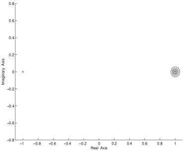
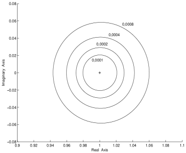
Refer to caption Refer to caption

Figure 1: The boundaries σε(P)subscript𝜎𝜀𝑃\,\partial\sigma_{\varepsilon}(P)\, for ε=104,2104,4104,8104𝜀superscript1042superscript1044superscript1048superscript104\,\varepsilon=10^{-4},2\cdot 10^{-4},4\cdot 10^{-4},8\cdot 10^{-4}.

The boundaries of the pseudospectra σε(P)subscript𝜎𝜀𝑃{\sigma}_{\varepsilon}(P), ε=104,2104,4104,8104,𝜀superscript1042superscript1044superscript1048superscript104\,\varepsilon=10^{-4},2\cdot 10^{-4},4\cdot 10^{-4},8\cdot 10^{-4},\, are illustrated in the left part of Figure 1. The eigenvalues of P(λ)𝑃𝜆P({\lambda}) are marked with ++’s and the components of the simple eigenvalue λ=1𝜆1{\lambda}=-1 are not visible. The components of the multiple eigenvalue λ=1𝜆1{\lambda}=1 are magnified in the right part of the figure, and they are very close to circular discs centered at λ=1𝜆1{\lambda}=1 of radii (k^(P,1) 104)1/2=0.0206superscript^𝑘𝑃1superscript104120.0206\,(\hat{k}(P,1)\,10^{-4})^{1/2}=0.0206, (k^(P,1) 2104)1/2=0.0291superscript^𝑘𝑃12superscript104120.0291(\hat{k}(P,1)\,2\cdot 10^{-4})^{1/2}=0.0291, (k^(P,1) 4104)1/2=0.0412superscript^𝑘𝑃14superscript104120.0412(\hat{k}(P,1)\,4\cdot 10^{-4})^{1/2}=0.0412\, and (k^(P,1) 8104)1/2=0.0583,superscript^𝑘𝑃18superscript104120.0583\,(\hat{k}(P,1)\,8\cdot 10^{-4})^{1/2}=0.0583,\, confirming Theorem 2.

4 Distance from a given simple eigenvalue to multiplicity

Let P(λ)𝑃𝜆P({\lambda}) be a matrix polynomial as in (1), and let λ0subscript𝜆0{\lambda}_{0} be a simple eigenvalue of P(λ)𝑃𝜆P({\lambda}). In the sequel, we generalize a methodology of Wilkinson [27] in order to obtain a relation between the condition number k(P,λ0)𝑘𝑃subscript𝜆0k(P,{\lambda}_{0}) and the distance from P(λ)𝑃𝜆P({\lambda}) to the matrix polynomials that have λ0subscript𝜆0{\lambda}_{0} as a multiple eigenvalue, namely,

dist(P,λ0)=inf{ε>0:Q(λ)(P,ε,w)with λ0 as a multiple eigenvalue}.dist𝑃subscript𝜆0infimumconditional-set𝜀0𝑄𝜆𝑃𝜀wwith λ0 as a multiple eigenvalue\textup{dist}(P,{\lambda}_{0})\,=\,\inf\left\{\varepsilon>0:\exists\;Q({\lambda})\in{\mathcal{B}}(P,\varepsilon,\textup{w})\;\mbox{with ${\lambda}_{0}$ as a multiple eigenvalue}\right\}.

The next proposition is a known result (see [2, Theorem 3.2] and [4, Proposition 16]). Here, we give a new proof, which motivates the proof of the main result of this section (Theorem 4) and is necessary for the remainder.

Proposition 3.

Let P(λ)𝑃𝜆P({\lambda}) be a matrix polynomial as in (1), λ0σ(P)\σ(P)subscript𝜆0\𝜎𝑃𝜎superscript𝑃{\lambda}_{0}\in{\sigma}(P)\backslash{\sigma}(P^{\prime}) and y0,x0nsubscript𝑦0subscript𝑥0superscript𝑛y_{0},x_{0}\in\mathbb{C}^{n} be corresponding left and right unit eigenvectors, respectively. If y0P(λ0)x0superscriptsubscript𝑦0superscript𝑃subscript𝜆0subscript𝑥0\,y_{0}^{*}P^{\prime}({\lambda}_{0})x_{0} =0,absent0=0,\, then λ0subscript𝜆0{\lambda}_{0} is a multiple eigenvalue of P(λ)𝑃𝜆P({\lambda}).

Proof.

By Schur’s triangularization, and without loss of generality, we may assume that the matrix P(λ0)𝑃subscript𝜆0P({\lambda}_{0}) has the following form,

P(λ0)=[0b0B];bn1,B(n1)×(n1).formulae-sequence𝑃subscript𝜆0delimited-[]0superscript𝑏0𝐵formulae-sequence𝑏superscript𝑛1𝐵superscript𝑛1𝑛1P({\lambda}_{0})=\left[\begin{array}[]{cc}0&b^{*}\\ 0&B\end{array}\right]\;;\;\;\;b\in\mathbb{C}^{n-1},\,\,B\in\mathbb{C}^{(n-1)\times(n-1)}.

Moreover, since P(λ0)x0=0𝑃subscript𝜆0subscript𝑥00P({\lambda}_{0})x_{0}=0, we can set x0=e1=[ 1  0 0]Tsubscript𝑥0subscript𝑒1superscriptdelimited-[]10 0𝑇x_{0}=e_{1}=\left[\,1\;\,0\;\cdots\;0\,\right]^{T}. Then we have that y0P(λ0)e1=0,superscriptsubscript𝑦0superscript𝑃subscript𝜆0subscript𝑒10\,y_{0}^{*}P^{\prime}({\lambda}_{0})e_{1}=0,\, and hence, y0P(λ0)=[0w]superscriptsubscript𝑦0superscript𝑃subscript𝜆0delimited-[]0superscript𝑤\,y_{0}^{*}P^{\prime}({\lambda}_{0})\,=\,[0\,\,w^{*}]\, for some  0wn1 0𝑤superscript𝑛1\,0\neq w\in\mathbb{C}^{n-1}.

Since λ0σ(P)subscript𝜆0𝜎superscript𝑃{\lambda}_{0}\notin{\sigma}(P^{\prime}) and y0P(λ0)=0superscriptsubscript𝑦0𝑃subscript𝜆00y_{0}^{*}P({\lambda}_{0})=0, it follows

y0P(λ0){[P(λ0)]1P(λ0)}= 0,superscriptsubscript𝑦0superscript𝑃subscript𝜆0superscriptdelimited-[]superscript𝑃subscript𝜆01𝑃subscript𝜆0 0y_{0}^{*}P^{\prime}({\lambda}_{0})\left\{[P^{\prime}({\lambda}_{0})]^{-1}P({\lambda}_{0})\right\}\,=\,0,

or equivalently,

y0P(λ0){[P(λ0)]1[0b0B]}= 0,superscriptsubscript𝑦0superscript𝑃subscript𝜆0superscriptdelimited-[]superscript𝑃subscript𝜆01delimited-[]0superscript𝑏0𝐵 0y_{0}^{*}P^{\prime}({\lambda}_{0})\left\{[P^{\prime}({\lambda}_{0})]^{-1}\left[\begin{array}[]{cc}0&b^{*}\\ 0&B\end{array}\right]\right\}\,=\,0,

or equivalently,

[0w][0a0A]= 0,delimited-[]0superscript𝑤delimited-[]0superscript𝑎0𝐴 0[0\,\,w^{*}]\left[\begin{array}[]{cc}0&a^{*}\\ 0&A\end{array}\right]\,=\,0,

where an1𝑎superscript𝑛1\,a\in\mathbb{C}^{n-1}\, and A(n1)×(n1)𝐴superscript𝑛1𝑛1\,A\in\mathbb{C}^{(n-1)\times(n-1)}. As a consequence, wA=0superscript𝑤𝐴0\,w^{*}A=0\, and the matrix A𝐴A has 00 as an eigenvalue. Thus, 00 is a multiple eigenvalue of the matrix [P(λ0)]1P(λ0)superscriptdelimited-[]superscript𝑃subscript𝜆01𝑃subscript𝜆0[P^{\prime}({\lambda}_{0})]^{-1}P({\lambda}_{0}). We consider two cases:

(i) If the geometric multiplicity of  0σ([P(λ0)]1P(λ0)) 0𝜎superscriptdelimited-[]superscript𝑃subscript𝜆01𝑃subscript𝜆0\,0\in{\sigma}([P^{\prime}({\lambda}_{0})]^{-1}P({\lambda}_{0})) is greater than or equal to 222, then rank(P(λ0))n2rank𝑃subscript𝜆0𝑛2\,\textup{rank}(P({\lambda}_{0}))\leq n-2, and hence, λ0subscript𝜆0{\lambda}_{0} is a multiple eigenvalue of P(λ)𝑃𝜆P({\lambda}).

(ii) Suppose that the geometric multiplicity of the eigenvalue  0σ([P(λ0)]1P(λ0)) 0𝜎superscriptdelimited-[]superscript𝑃subscript𝜆01𝑃subscript𝜆0\,0\in{\sigma}([P^{\prime}({\lambda}_{0})]^{-1}P({\lambda}_{0})) is equal to 111 and its algebraic multiplicity is greater than or equal to 222. Then, keeping in mind that [P(λ0)]1P(λ0)e1=0,superscriptdelimited-[]superscript𝑃subscript𝜆01𝑃subscript𝜆0subscript𝑒10\,[P^{\prime}({\lambda}_{0})]^{-1}P({\lambda}_{0})e_{1}=0,\, we verify that there exists a vector z1nsubscript𝑧1superscript𝑛z_{1}\in\mathbb{C}^{n} such that [P(λ0)]1P(λ0)z1=e1,superscriptdelimited-[]superscript𝑃subscript𝜆01𝑃subscript𝜆0subscript𝑧1subscript𝑒1\,[P^{\prime}({\lambda}_{0})]^{-1}P({\lambda}_{0})z_{1}=e_{1},\, or equivalently, P(λ0)(z1)+P(λ0)e1=0𝑃subscript𝜆0subscript𝑧1superscript𝑃subscript𝜆0subscript𝑒10\,P({\lambda}_{0})(-z_{1})+P^{\prime}({\lambda}_{0})e_{1}=0. Thus, λ0subscript𝜆0{\lambda}_{0} is a multiple eigenvalue of P(λ)𝑃𝜆P({\lambda}) with a Jordan chain of length at least 222. ∎

Recall that the condition number of an invertible matrix A𝐴A is defined by c(A)=AA1𝑐𝐴norm𝐴normsuperscript𝐴1c(A)=\|A\|\,\|A^{-1}\| and it is always greater than or equal to 111.

Theorem 4.

Let P(λ)𝑃𝜆P({\lambda}) be a matrix polynomial as in (1), λ0σ(P)\σ(P)subscript𝜆0\𝜎𝑃𝜎superscript𝑃{\lambda}_{0}\in{\sigma}(P)\backslash{\sigma}(P^{\prime}) be a simple eigenvalue of P(λ)𝑃𝜆P({\lambda}), and y0,x0nsubscript𝑦0subscript𝑥0superscript𝑛y_{0},x_{0}\in\mathbb{C}^{n} be corresponding left and right unit eigenvectors, respectively. If the vector [P(λ0)]y0superscriptdelimited-[]superscript𝑃subscript𝜆0subscript𝑦0[P^{\prime}({\lambda}_{0})]^{*}y_{0} is not a scalar multiple of x0subscript𝑥0x_{0}, then

dist(P,λ0)c(P(λ0))P(λ0)k(P,λ0)(y0P(λ0)2|y0P(λ0)x0|2)1/2.dist𝑃subscript𝜆0𝑐superscript𝑃subscript𝜆0norm𝑃subscript𝜆0𝑘𝑃subscript𝜆0superscriptsuperscriptnormsuperscriptsubscript𝑦0superscript𝑃subscript𝜆02superscriptsuperscriptsubscript𝑦0superscript𝑃subscript𝜆0subscript𝑥0212\textup{dist}(P,{\lambda}_{0})\,\leq\,\frac{c(P^{\prime}({\lambda}_{0}))\,\left\|P({\lambda}_{0})\right\|}{k(P,{\lambda}_{0})\left(\left\|y_{0}^{*}P^{\prime}({\lambda}_{0})\right\|^{2}-|y_{0}^{*}P^{\prime}({\lambda}_{0})x_{0}|^{2}\right)^{1/2}}.
Proof.

As in the proof of the previous proposition, without loss of generality, we may assume that

P(λ0)=[0b0B];bn1,B(n1)×(n1)formulae-sequence𝑃subscript𝜆0delimited-[]0superscript𝑏0𝐵formulae-sequence𝑏superscript𝑛1𝐵superscript𝑛1𝑛1P({\lambda}_{0})=\left[\begin{array}[]{cc}0&b^{*}\\ 0&B\end{array}\right]\;;\;\;\;b\in\mathbb{C}^{n-1},\,\,B\in\mathbb{C}^{(n-1)\times(n-1)}

and x0=e1subscript𝑥0subscript𝑒1x_{0}=e_{1}. If we denote δ=y0P(λ0)x0=y0P(λ0)e10𝛿superscriptsubscript𝑦0superscript𝑃subscript𝜆0subscript𝑥0superscriptsubscript𝑦0superscript𝑃subscript𝜆0subscript𝑒10{\delta}=y_{0}^{*}P^{\prime}({\lambda}_{0})x_{0}=y_{0}^{*}P^{\prime}({\lambda}_{0})e_{1}\neq 0, then it is clear that

y0P(λ0)=[δw],superscriptsubscript𝑦0superscript𝑃subscript𝜆0delimited-[]𝛿superscript𝑤y_{0}^{*}P^{\prime}({\lambda}_{0})\,=\,\left[\,{\delta}\,\;w^{*}\right],

for some wn1𝑤superscript𝑛1\,w\in\mathbb{C}^{n-1}. Furthermore, w0𝑤0\,w\neq 0\, because |δ|<y0P(λ0)𝛿normsuperscriptsubscript𝑦0superscript𝑃subscript𝜆0\,|{\delta}|<\left\|y_{0}^{*}P^{\prime}({\lambda}_{0})\right\|.

Since λ0σ(P)subscript𝜆0𝜎superscript𝑃{\lambda}_{0}\notin{\sigma}(P^{\prime}) and y0P(λ0)=0superscriptsubscript𝑦0𝑃subscript𝜆00y_{0}^{*}P({\lambda}_{0})=0, it follows

y0P(λ0){[P(λ0)]1P(λ0)}= 0,superscriptsubscript𝑦0superscript𝑃subscript𝜆0superscriptdelimited-[]superscript𝑃subscript𝜆01𝑃subscript𝜆0 0y_{0}^{*}P^{\prime}({\lambda}_{0})\left\{[P^{\prime}({\lambda}_{0})]^{-1}P({\lambda}_{0})\right\}\,=\,0,

or equivalently,

y0P(λ0){[P(λ0)]1[0b0B]}= 0,superscriptsubscript𝑦0superscript𝑃subscript𝜆0superscriptdelimited-[]superscript𝑃subscript𝜆01delimited-[]0superscript𝑏0𝐵 0y_{0}^{*}P^{\prime}({\lambda}_{0})\left\{[P^{\prime}({\lambda}_{0})]^{-1}\left[\begin{array}[]{cc}0&b^{*}\\ 0&B\end{array}\right]\right\}\,=\,0,

or equivalently,

[δw][0a0A]= 0delimited-[]𝛿superscript𝑤delimited-[]0superscript𝑎0𝐴 0\left[{\delta}\,\,w^{*}\right]\left[\begin{array}[]{cc}0&a^{*}\\ 0&A\end{array}\right]\,=\,0

for some an1𝑎superscript𝑛1\,a\in\mathbb{C}^{n-1}\, and A(n1)×(n1)𝐴superscript𝑛1𝑛1\,A\in\mathbb{C}^{(n-1)\times(n-1)}. If a=0𝑎0a=0, then wA=0superscript𝑤𝐴0w^{*}A=0, and the proof of Proposition 3 implies that λ0subscript𝜆0{\lambda}_{0} is a multiple eigenvalue of P(λ)𝑃𝜆P({\lambda}); this is a contradiction. As a consequence, a0𝑎0a\neq 0. Moreover,

wA+δa= 0,superscript𝑤𝐴𝛿superscript𝑎 0w^{*}A+{\delta}a^{*}\,=\,0,

and hence,

w(A+δwwwa)= 0.superscript𝑤𝐴𝛿superscript𝑤𝑤𝑤superscript𝑎 0w^{*}\left(A+\frac{{\delta}}{w^{*}w}wa^{*}\right)\,=\,0.

This means that if we consider the (perturbation) matrix E=[000δwwwa],𝐸delimited-[]000𝛿superscript𝑤𝑤𝑤superscript𝑎\,E=\left[\begin{array}[]{cc}0&0\\ 0&\frac{{\delta}}{w^{*}w}wa^{*}\end{array}\right],\, then the matrix

[P(λ0)]1P(λ0)+E=[P(λ0)]1[P(λ0)+P(λ0)E]superscriptdelimited-[]superscript𝑃subscript𝜆01𝑃subscript𝜆0𝐸superscriptdelimited-[]superscript𝑃subscript𝜆01delimited-[]𝑃subscript𝜆0superscript𝑃subscript𝜆0𝐸[P^{\prime}({\lambda}_{0})]^{-1}P({\lambda}_{0})+E\,=\,[P^{\prime}({\lambda}_{0})]^{-1}\left[P({\lambda}_{0})+P^{\prime}({\lambda}_{0})E\right]

has  0 0\,0\, as a multiple eigenvalue.

We define the n×n𝑛𝑛n\times n matrices

Δ^=P(λ0)EandQ^=P(λ0)+Δ^,^Δsuperscript𝑃subscript𝜆0𝐸and^𝑄𝑃subscript𝜆0^Δ\hat{\Delta}\,=\,P^{\prime}({\lambda}_{0})E\;\;\;\mbox{and}\;\;\;\hat{Q}=P({\lambda}_{0})+\hat{\Delta},

and the matrix polynomial Δ(λ)=j=0mΔjλjΔ𝜆superscriptsubscript𝑗0𝑚subscriptΔ𝑗superscript𝜆𝑗\,{\Delta}({\lambda})=\sum_{j=0}^{m}{\Delta}_{j}{\lambda}^{j}\, with coefficients

Δj=(λ0¯|λ0|)jwjw(|λ0|)Δ^;j=0,1,,m,formulae-sequencesubscriptΔ𝑗superscript¯subscript𝜆0subscript𝜆0𝑗subscript𝑤𝑗𝑤subscript𝜆0^Δ𝑗01𝑚{\Delta}_{j}\,=\,\left(\frac{\overline{{\lambda}_{0}}}{|{\lambda}_{0}|}\right)^{j}\frac{w_{j}}{w(|{\lambda}_{0}|)}\,\hat{\Delta}\;;\;\;\;j=0,1,\dots,m,

where (by convention) we assume that λ0¯/λ0=0¯subscript𝜆0subscript𝜆00\overline{{\lambda}_{0}}/{\lambda}_{0}=0 whenever λ0=0subscript𝜆00{\lambda}_{0}=0. Then, denoting ϕ=w(|λ0|)w(|λ0|)λ0¯|λ0|italic-ϕsuperscript𝑤subscript𝜆0𝑤subscript𝜆0¯subscript𝜆0subscript𝜆0\phi=\frac{w^{\prime}(|{\lambda}_{0}|)}{w(|{\lambda}_{0}|)}\frac{\overline{{\lambda}_{0}}}{|{\lambda}_{0}|}, one can verify that

Δ(λ0)=Δ^andΔ(λ0)=ϕΔ^.Δsubscript𝜆0^ΔandsuperscriptΔsubscript𝜆0italic-ϕ^Δ{\Delta}({\lambda}_{0})\,=\,\hat{\Delta}\;\;\;\mbox{and}\;\;\;{\Delta}^{\prime}({\lambda}_{0})\,=\,\phi\hat{\Delta}.

We define also the matrix polynomial Q(λ)=P(λ)+Δ(λ),𝑄𝜆𝑃𝜆Δ𝜆\,Q({\lambda})=P({\lambda})+{\Delta}({\lambda}),\, and consider two cases:

(i) Suppose that the geometric multiplicity of  0σ([P(λ0)]1Q^) 0𝜎superscriptdelimited-[]superscript𝑃subscript𝜆01^𝑄\,0\in{\sigma}([P^{\prime}({\lambda}_{0})]^{-1}\hat{Q}) is greater than or equal to 222. Then rank(Q^)=rank(Q(λ0))n2,rank^𝑄rank𝑄subscript𝜆0𝑛2\,\textup{rank}(\hat{Q})=\textup{rank}(Q({\lambda}_{0}))\leq n-2,\, or equivalently, λ0subscript𝜆0{\lambda}_{0} is a multiple eigenvalue of the matrix polynomial Q(λ)𝑄𝜆Q({\lambda}) of geometric multiplicity at least 222.

(ii) Suppose now that the geometric multiplicity of the eigenvalue  0σ([P(λ0)]1Q^) 0𝜎superscriptdelimited-[]superscript𝑃subscript𝜆01^𝑄\,0\in{\sigma}([P^{\prime}({\lambda}_{0})]^{-1}\hat{Q})\, is equal to 111, and its algebraic multiplicity is greater than or equal to 222. Then, keeping in mind that Q^e1=0^𝑄subscript𝑒10\hat{Q}e_{1}=0, there is a vector z1nsubscript𝑧1superscript𝑛z_{1}\in\mathbb{C}^{n} such that

[P(λ0)]1Q^z1=e1,superscriptdelimited-[]superscript𝑃subscript𝜆01^𝑄subscript𝑧1subscript𝑒1[P^{\prime}({\lambda}_{0})]^{-1}\hat{Q}z_{1}\,=\,e_{1},

or equivalently,

Q^(z1)+P(λ0)e1= 0.^𝑄subscript𝑧1superscript𝑃subscript𝜆0subscript𝑒1 0\hat{Q}(-z_{1})+P^{\prime}({\lambda}_{0})e_{1}\,=\,0. (12)

We observe that Δ(λ0)e1=ϕΔ^e1=ϕP(λ0)Ee1=0superscriptΔsubscript𝜆0subscript𝑒1italic-ϕ^Δsubscript𝑒1italic-ϕsuperscript𝑃subscript𝜆0𝐸subscript𝑒10\,{\Delta}^{\prime}({\lambda}_{0})e_{1}=\phi\hat{\Delta}e_{1}=\phi P^{\prime}({\lambda}_{0})Ee_{1}=0. As a consequence, (12) is written in the form

Q(λ0)(z1)+Q(λ0)e1= 0.𝑄subscript𝜆0subscript𝑧1superscript𝑄subscript𝜆0subscript𝑒1 0Q({\lambda}_{0})(-z_{1})+Q^{\prime}({\lambda}_{0})e_{1}\,=\,0.

Thus, λ0subscript𝜆0{\lambda}_{0} is a multiple eigenvalue of Q(λ)𝑄𝜆Q({\lambda}) with a Jordan chain of length at least 222.

In both cases above, we have proved that λ0subscript𝜆0{\lambda}_{0} is a multiple eigenvalue of Q(λ)𝑄𝜆Q({\lambda}). Furthermore, we see that

Enorm𝐸\displaystyle\left\|E\right\| =\displaystyle= [000δwwwa]=δwwwa=|δ|wanormdelimited-[]000𝛿superscript𝑤𝑤𝑤superscript𝑎norm𝛿superscript𝑤𝑤𝑤superscript𝑎𝛿norm𝑤norm𝑎\displaystyle\left\|\left[\begin{array}[]{cc}0&0\\ 0&\frac{{\delta}}{w^{*}w}wa^{*}\end{array}\right]\right\|=\left\|\frac{{\delta}}{w^{*}w}wa^{*}\right\|=\frac{|{\delta}|}{\left\|w\right\|}\left\|a\right\|
\displaystyle\leq |δ|w[0a0A]=|δ|w[P(λ0)]1P(λ0)𝛿norm𝑤normdelimited-[]0𝑎0𝐴𝛿norm𝑤normsuperscriptdelimited-[]superscript𝑃subscript𝜆01𝑃subscript𝜆0\displaystyle\frac{|{\delta}|}{\left\|w\right\|}\left\|\left[\begin{array}[]{cc}0&a\\ 0&A\end{array}\right]\right\|=\frac{|{\delta}|}{\left\|w\right\|}\left\|[P^{\prime}({\lambda}_{0})]^{-1}P({\lambda}_{0})\right\|
\displaystyle\leq |δ|w[P(λ0)]1P(λ0).𝛿norm𝑤normsuperscriptdelimited-[]superscript𝑃subscript𝜆01norm𝑃subscript𝜆0\displaystyle\frac{|{\delta}|}{\left\|w\right\|}\left\|[P^{\prime}({\lambda}_{0})]^{-1}\right\|\left\|P({\lambda}_{0})\right\|.

As a consequence, for every j=0,1,,m𝑗01𝑚\,j=0,1,\dots,m,

ΔjnormsubscriptΔ𝑗\displaystyle\left\|{\Delta}_{j}\right\| =\displaystyle= wjw(|λ0|)Δ^=wjw(|λ0|)P(λ0)Esubscript𝑤𝑗𝑤subscript𝜆0norm^Δsubscript𝑤𝑗𝑤subscript𝜆0normsuperscript𝑃subscript𝜆0𝐸\displaystyle\frac{w_{j}}{w(|{\lambda}_{0}|)}\left\|\hat{{\Delta}}\right\|\,=\,\frac{w_{j}}{w(|{\lambda}_{0}|)}\left\|P^{\prime}({\lambda}_{0})E\right\|
\displaystyle\leq wjw(|λ0|)P(λ0)Esubscript𝑤𝑗𝑤subscript𝜆0normsuperscript𝑃subscript𝜆0norm𝐸\displaystyle\frac{w_{j}}{w(|{\lambda}_{0}|)}\left\|P^{\prime}({\lambda}_{0})\right\|\left\|E\right\|
\displaystyle\leq wjw(|λ0|)|δ|w[P(λ0)]1P(λ0)P(λ0)subscript𝑤𝑗𝑤subscript𝜆0𝛿norm𝑤normsuperscriptdelimited-[]superscript𝑃subscript𝜆01normsuperscript𝑃subscript𝜆0norm𝑃subscript𝜆0\displaystyle\frac{w_{j}}{w(|{\lambda}_{0}|)}\frac{|{\delta}|}{\left\|w\right\|}\left\|[P^{\prime}({\lambda}_{0})]^{-1}\right\|\left\|P^{\prime}({\lambda}_{0})\right\|\left\|P({\lambda}_{0})\right\|
=\displaystyle= wjc(P(λ0))P(λ0)k(P,λ0)(y0P(λ0)2δ2)1/2,subscript𝑤𝑗𝑐superscript𝑃subscript𝜆0norm𝑃subscript𝜆0𝑘𝑃subscript𝜆0superscriptsuperscriptnormsuperscriptsubscript𝑦0superscript𝑃subscript𝜆02superscript𝛿212\displaystyle w_{j}\,\frac{c(P^{\prime}({\lambda}_{0}))\,\left\|P({\lambda}_{0})\right\|}{k(P,{\lambda}_{0})\left(\left\|y_{0}^{*}P^{\prime}({\lambda}_{0})\right\|^{2}-{\delta}^{2}\right)^{1/2}},

and the proof is complete. ∎

The spectrum of the matrix polynomial

P(λ)𝑃𝜆\displaystyle P({\lambda}) =\displaystyle= Iλ2+[102000.25000.5]λ+[008025i0015.25]𝐼superscript𝜆2delimited-[]102000.25000.5𝜆delimited-[]008025i0015.25\displaystyle I{\lambda}^{2}+\left[\begin{array}[]{ccc}1&0&2\\ 0&0&0.25\\ 0&0&-0.5\end{array}\right]{\lambda}+\left[\begin{array}[]{ccc}0&0&8\\ 0&25&-\textup{i}\\ 0&0&15.25\end{array}\right]

is σ(P)={0,1,0.25±i 3.8971,±i 5}𝜎𝑃01plus-or-minus0.25i3.8971plus-or-minusi5{\sigma}(P)=\{0,-1,0.25\pm\textup{i}\,3.8971,\pm\textup{i}\,5\}. For the weights w2=A2=1subscript𝑤2normsubscript𝐴21\,w_{2}=\left\|A_{2}\right\|=1, w1=A1=2.2919subscript𝑤1normsubscript𝐴12.2919w_{1}=\left\|A_{1}\right\|=2.2919 and w0=A0=25.0379,subscript𝑤0normsubscript𝐴025.0379w_{0}=\left\|A_{0}\right\|=25.0379,\, the above theorem implies dist(P,1)0.4991dist𝑃10.4991\,\textup{dist}(P,-1)\leq 0.4991. If we estimate the same distance using the method proposed in [18], then we see that dist(P,1)0.5991dist𝑃10.5991\,\textup{dist}(P,-1)\leq 0.5991. On the other hand, for the eigenvalue 0.25i 3.89710.25i3.89710.25-\textup{i}\,3.8971, Theorem 4 yields dist(P,0.25i 3.8971)0.1485dist𝑃0.25i3.89710.1485\,\textup{dist}(P,0.25-\textup{i}\,3.8971)\leq 0.1485, and the method of [18] implies dist(P,0.25i 3.8971)0.1398dist𝑃0.25i3.89710.1398\,\textup{dist}(P,0.25-\textup{i}\,3.8971)\leq 0.1398. At this point, it is necessary to remark that the methodology of [18] is applicable to every complex number and not only to simple eigenvalues of P(λ)𝑃𝜆P({\lambda}).

5 An expression of k(P,λ0)𝑘𝑃subscript𝜆0k(P,{\lambda}_{0}) without eigenvectors

In this section, we derive a new expression of the condition number k(P,λ0)𝑘𝑃subscript𝜆0k(P,{\lambda}_{0}) that involves the distances from λ0σ(P)subscript𝜆0𝜎𝑃{\lambda}_{0}\in{\sigma}(P) to the rest of the eigenvalues of the matrix polynomial P(λ)𝑃𝜆P({\lambda}), instead of the left and right eigenvectors of λ0subscript𝜆0{\lambda}_{0}. The next three lemmas are necessary for our discussion. The first lemma is part of the proof of Theorem 2 in [20], the second lemma follows readily from the singular value decomposition, and the third lemma is part of Theorem 4 in [20].

Lemma 5.

For any matrices C,R,Wn×n𝐶𝑅𝑊superscript𝑛𝑛\,C,R,W\in\mathbb{C}^{n\times n}, Radj(WCR)W=det(WR)adj(C)𝑅adj𝑊𝐶𝑅𝑊𝑊𝑅adj𝐶\,R\,\textup{adj}(WCR)\,W=\det(WR)\,\textup{adj}(C).

Lemma 6.

Let A𝐴A be an n×n𝑛𝑛n\times n matrix with 00 as a simple eigenvalue, s1s2sn1>sn=0subscript𝑠1subscript𝑠2subscript𝑠𝑛1subscript𝑠𝑛0\,s_{1}\geq s_{2}\geq\dots\geq s_{n-1}>s_{n}=0\, be the singular values of A𝐴A, and un,vnnsubscript𝑢𝑛subscript𝑣𝑛superscript𝑛u_{n},v_{n}\in\mathbb{C}^{n} be left and right singular vectors of sn=0subscript𝑠𝑛0s_{n}=0, respectively. Then unsubscript𝑢𝑛u_{n} and vnsubscript𝑣𝑛v_{n} are also left and right eigenvectors of A𝐴A corresponding to 00, respectively.

Lemma 7.

Let A𝐴A be an n×n𝑛𝑛n\times n matrix with 00 as a simple eigenvalue. If s1s2sn1>sn=0subscript𝑠1subscript𝑠2subscript𝑠𝑛1subscript𝑠𝑛0\,s_{1}\geq s_{2}\geq\dots\geq s_{n-1}>s_{n}=0\, are the singular values of A𝐴A, then adj(A)=s1s2sn1normadj𝐴subscript𝑠1subscript𝑠2subscript𝑠𝑛1\,\left\|\textup{adj}(A)\right\|=s_{1}s_{2}\cdots s_{n-1}.

The following theorem is a direct generalization of Theorem 2 of [20].

Theorem 8.

Let P(λ)𝑃𝜆P({\lambda}) be a matrix polynomial as in (1) with spectrum σ(P)={λ1,λ2,,λnm}𝜎𝑃subscript𝜆1subscript𝜆2subscript𝜆𝑛𝑚{\sigma}(P)=\{{\lambda}_{1},{\lambda}_{2},\dots,{\lambda}_{nm}\}, counting algebraic multiplicities. If λisubscript𝜆𝑖{\lambda}_{i} is a simple eigenvalue, then

k(P,λi)=w(|λi|)adj(P(λi))|detAm|ji|λjλi|.𝑘𝑃subscript𝜆𝑖𝑤subscript𝜆𝑖normadj𝑃subscript𝜆𝑖subscript𝐴𝑚subscriptproduct𝑗𝑖subscript𝜆𝑗subscript𝜆𝑖k(P,{\lambda}_{i})\,=\,\frac{w(\left|{\lambda}_{i}\right|)\,\left\|\textup{adj}(P({\lambda}_{i}))\right\|}{|\det A_{m}|\,\prod_{j\neq i}|{\lambda}_{j}-{\lambda}_{i}|}.
Proof.

For the simple eigenvalue λiσ(P)subscript𝜆𝑖𝜎𝑃{\lambda}_{i}\in{\sigma}(P), consider a singular value decomposition of matrix P(λi)𝑃subscript𝜆𝑖P({\lambda}_{i}),

P(λi)=UΣV=Udiag{s1,,sn1,0}V.𝑃subscript𝜆𝑖𝑈Σsuperscript𝑉𝑈diagsubscript𝑠1subscript𝑠𝑛10superscript𝑉P({\lambda}_{i})\,=\,U\,{\Sigma}\,V^{*}\,=\,U\textup{diag}\{s_{1},\dots,s_{n-1},0\}\,V^{*}.

Then we have

[U00In(m1)][P(λi)00In(m1)][V00In(m1)]=[Σ00In(m1)],delimited-[]superscript𝑈00subscript𝐼𝑛𝑚1delimited-[]𝑃subscript𝜆𝑖0missing-subexpressionmissing-subexpression0subscript𝐼𝑛𝑚1missing-subexpressionmissing-subexpressiondelimited-[]𝑉0missing-subexpressionmissing-subexpression0subscript𝐼𝑛𝑚1missing-subexpressionmissing-subexpressiondelimited-[]Σ0missing-subexpressionmissing-subexpression0subscript𝐼𝑛𝑚1missing-subexpressionmissing-subexpression\left[\begin{array}[]{cc}U^{*}&0\\ 0&I_{n(m-1)}\end{array}\right]\left[\begin{array}[]{cccc}P({\lambda}_{i})&0\\ 0&I_{n(m-1)}\end{array}\right]\left[\begin{array}[]{cccc}V&0\\ 0&I_{n(m-1)}\end{array}\right]=\left[\begin{array}[]{cccc}{\Sigma}&0\\ 0&I_{n(m-1)}\end{array}\right],

and Lemma 5 implies

[V00In(m1)]adj([Σ00In(m1)])[U00In(m1)]delimited-[]𝑉0missing-subexpressionmissing-subexpression0subscript𝐼𝑛𝑚1missing-subexpressionmissing-subexpressionadjdelimited-[]Σ0missing-subexpressionmissing-subexpression0subscript𝐼𝑛𝑚1missing-subexpressionmissing-subexpressiondelimited-[]superscript𝑈0missing-subexpressionmissing-subexpression0subscript𝐼𝑛𝑚1missing-subexpressionmissing-subexpression\left[\begin{array}[]{cccc}V&0\\ 0&I_{n(m-1)}\end{array}\right]\textup{adj}\left(\left[\begin{array}[]{cccc}{\Sigma}&0\\ 0&I_{n(m-1)}\end{array}\right]\right)\left[\begin{array}[]{cccc}U^{*}&0\\ 0&I_{n(m-1)}\end{array}\right] (16)
=det(UV)adj([P(λ0)00In(m1)]),absentsuperscript𝑈𝑉adjdelimited-[]𝑃subscript𝜆00missing-subexpressionmissing-subexpression0subscript𝐼𝑛𝑚1missing-subexpressionmissing-subexpression\,=\,\det(U^{*}V)\,\textup{adj}\left(\left[\begin{array}[]{cccc}P({\lambda}_{0})&0\\ 0&I_{n(m-1)}\end{array}\right]\right),

where |det(UV)|=1superscript𝑈𝑉1|\det(U^{*}V)|=1.

Let un,vnnsubscript𝑢𝑛subscript𝑣𝑛superscript𝑛u_{n},v_{n}\in\mathbb{C}^{n} be the last columns of U𝑈U and V𝑉V, respectively, i.e., they are left and right singular vectors of the zero singular value of P(λi)𝑃subscript𝜆𝑖P({\lambda}_{i}). Then by Lemma 6, yi=unsubscript𝑦𝑖subscript𝑢𝑛y_{i}=u_{n} and xi=vnsubscript𝑥𝑖subscript𝑣𝑛x_{i}=v_{n} are left and right unit eigenvectors of λiσ(P)subscript𝜆𝑖𝜎𝑃\,{\lambda}_{i}\in{\sigma}(P), respectively. Let also ψisubscript𝜓𝑖\psi_{i} and χisubscript𝜒𝑖\chi_{i} be the associated left and right eigenvectors of CPsubscript𝐶𝑃C_{P} for the eigenvalue λisubscript𝜆𝑖{\lambda}_{i} given by (7). Then by (8), [20, Theorem 2], Lemma 5, (2) and (16) (applied in this specific order), it follows

k(P,λi)𝑘𝑃subscript𝜆𝑖\displaystyle k(P,{\lambda}_{i}) =\displaystyle= w(|λi|)χiψik(CP,λi)𝑤subscript𝜆𝑖normsubscript𝜒𝑖normsubscript𝜓𝑖𝑘subscript𝐶𝑃subscript𝜆𝑖\displaystyle\frac{w(\left|{\lambda}_{i}\right|)}{\left\|\chi_{i}\right\|\left\|\psi_{i}\right\|}\,k(C_{P},{\lambda}_{i})
=\displaystyle= w(|λi|)χiψiadj(λiICP)ji|λjλi|𝑤subscript𝜆𝑖normsubscript𝜒𝑖normsubscript𝜓𝑖normadjsubscript𝜆𝑖𝐼subscript𝐶𝑃subscriptproduct𝑗𝑖subscript𝜆𝑗subscript𝜆𝑖\displaystyle\frac{w(\left|{\lambda}_{i}\right|)}{\left\|\chi_{i}\right\|\left\|\psi_{i}\right\|}\frac{\left\|\textup{adj}({\lambda}_{i}I-C_{P})\right\|}{\prod_{j\neq i}|{\lambda}_{j}-{\lambda}_{i}|}
=\displaystyle= w(|λi|)χiψiF(λi)adj(E(λi)(λiICP)F(λi))E(λi)|det(F(λi)E(λi))|ji|λjλi|𝑤subscript𝜆𝑖normsubscript𝜒𝑖normsubscript𝜓𝑖norm𝐹subscript𝜆𝑖adj𝐸subscript𝜆𝑖subscript𝜆𝑖𝐼subscript𝐶𝑃𝐹subscript𝜆𝑖𝐸subscript𝜆𝑖𝐹subscript𝜆𝑖𝐸subscript𝜆𝑖subscriptproduct𝑗𝑖subscript𝜆𝑗subscript𝜆𝑖\displaystyle\frac{w(\left|{\lambda}_{i}\right|)}{\left\|\chi_{i}\right\|\left\|\psi_{i}\right\|}\frac{\left\|F({\lambda}_{i})\,\,\textup{adj}(E({\lambda}_{i})({\lambda}_{i}I-C_{P})F({\lambda}_{i}))\,E({\lambda}_{i})\right\|}{|\det(F({\lambda}_{i})E({\lambda}_{i}))|\,\prod_{j\neq i}|{\lambda}_{j}-{\lambda}_{i}|}
=\displaystyle= w(|λi|)χiψiF(λi)adj([P(λi)00In(m1)])E(λi)|det(F(λi)E(λi))|ji|λjλi|𝑤subscript𝜆𝑖normsubscript𝜒𝑖normsubscript𝜓𝑖norm𝐹subscript𝜆𝑖adjdelimited-[]𝑃subscript𝜆𝑖00subscript𝐼𝑛𝑚1𝐸subscript𝜆𝑖𝐹subscript𝜆𝑖𝐸subscript𝜆𝑖subscriptproduct𝑗𝑖subscript𝜆𝑗subscript𝜆𝑖\displaystyle\frac{w(\left|{\lambda}_{i}\right|)}{\left\|\chi_{i}\right\|\left\|\psi_{i}\right\|}\frac{\left\|F({\lambda}_{i})\,\,\textup{adj}\left(\left[\begin{array}[]{cc}P({\lambda}_{i})&0\\ 0&I_{n(m-1)}\\ \end{array}\right]\right)E({\lambda}_{i})\right\|}{|\det(F({\lambda}_{i})E({\lambda}_{i}))|\,\prod_{j\neq i}|{\lambda}_{j}-{\lambda}_{i}|}
=\displaystyle= w(|λi|)χiψiF(λi)[V00In(m1)]adj([Σ00In(m1)])[U00In(m1)]E(λi)|detAm|ji|λjλi|.𝑤subscript𝜆𝑖normsubscript𝜒𝑖normsubscript𝜓𝑖norm𝐹subscript𝜆𝑖delimited-[]𝑉00subscript𝐼𝑛𝑚1adjdelimited-[]Σ00subscript𝐼𝑛𝑚1delimited-[]superscript𝑈00subscript𝐼𝑛𝑚1𝐸subscript𝜆𝑖subscript𝐴𝑚subscriptproduct𝑗𝑖subscript𝜆𝑗subscript𝜆𝑖\displaystyle\frac{w(\left|{\lambda}_{i}\right|)}{\left\|\chi_{i}\right\|\left\|\psi_{i}\right\|}\frac{\left\|F({\lambda}_{i})\left[\begin{array}[]{cc}V&0\\ 0&I_{n(m-1)}\end{array}\right]\textup{adj}\left(\left[\begin{array}[]{cc}{\Sigma}&0\\ 0&I_{n(m-1)}\end{array}\right]\right)\left[\begin{array}[]{cc}U^{*}&0\\ 0&I_{n(m-1)}\end{array}\right]E({\lambda}_{i})\right\|}{|\det A_{m}|\,\prod_{j\neq i}|{\lambda}_{j}-{\lambda}_{i}|}.

Thus,

k(P,λi)=w(|λi|)Gχiψi|detAm|ji|λjλi|,𝑘𝑃subscript𝜆𝑖𝑤subscript𝜆𝑖norm𝐺normsubscript𝜒𝑖normsubscript𝜓𝑖subscript𝐴𝑚subscriptproduct𝑗𝑖subscript𝜆𝑗subscript𝜆𝑖k(P,{\lambda}_{i})\,=\,\frac{w(\left|{\lambda}_{i}\right|)\,\left\|G\right\|}{\left\|\chi_{i}\right\|\left\|\psi_{i}\right\|\,|\det A_{m}|\,\prod_{j\neq i}|{\lambda}_{j}-{\lambda}_{i}|}, (19)

where

G=F(λi)[V00In(m1)]adj([Σ00In(m1)])[U00In(m1)]E(λi).𝐺𝐹subscript𝜆𝑖delimited-[]𝑉0missing-subexpressionmissing-subexpression0subscript𝐼𝑛𝑚1missing-subexpressionmissing-subexpressionadjdelimited-[]Σ0missing-subexpressionmissing-subexpression0subscript𝐼𝑛𝑚1missing-subexpressionmissing-subexpressiondelimited-[]superscript𝑈0missing-subexpressionmissing-subexpression0subscript𝐼𝑛𝑚1missing-subexpressionmissing-subexpression𝐸subscript𝜆𝑖G\,=\,F({\lambda}_{i})\left[\begin{array}[]{cccc}V&0\\ 0&I_{n(m-1)}\end{array}\right]\textup{adj}\left(\left[\begin{array}[]{cccc}{\Sigma}&0\\ 0&I_{n(m-1)}\end{array}\right]\right)\left[\begin{array}[]{cccc}U^{*}&0\\ 0&I_{n(m-1)}\end{array}\right]E({\lambda}_{i}).

Moreover,

adj([Σ00In(m1)])=[S000n(m1)],adjdelimited-[]Σ0missing-subexpressionmissing-subexpression0subscript𝐼𝑛𝑚1missing-subexpressionmissing-subexpressiondelimited-[]𝑆0missing-subexpressionmissing-subexpression0subscript0𝑛𝑚1missing-subexpressionmissing-subexpression\textup{adj}\left(\left[\begin{array}[]{cccc}{\Sigma}&0\\ 0&I_{n(m-1)}\end{array}\right]\right)\,=\,\left[\begin{array}[]{cccc}S&0\\ 0&0_{n(m-1)}\end{array}\right],

where S=s1s2sn1diag{0,,0,1}𝑆subscript𝑠1subscript𝑠2subscript𝑠𝑛1diag001S=s_{1}s_{2}\cdots s_{n-1}\textup{diag}\{0,\dots,0,1\}. As a consequence, the matrix G𝐺G is written

G𝐺\displaystyle G =\displaystyle= F(λi)[V00In(m1)][S000n(m1)][U00In(m1)]E(λi)𝐹subscript𝜆𝑖delimited-[]𝑉0missing-subexpressionmissing-subexpression0subscript𝐼𝑛𝑚1missing-subexpressionmissing-subexpressiondelimited-[]𝑆0missing-subexpressionmissing-subexpression0subscript0𝑛𝑚1missing-subexpressionmissing-subexpressiondelimited-[]superscript𝑈0missing-subexpressionmissing-subexpression0subscript𝐼𝑛𝑚1missing-subexpressionmissing-subexpression𝐸subscript𝜆𝑖\displaystyle F({\lambda}_{i})\,\,\left[\begin{array}[]{cccc}V&0\\ 0&I_{n(m-1)}\end{array}\right]\left[\begin{array}[]{cccc}S&0\\ 0&0_{n(m-1)}\end{array}\right]\left[\begin{array}[]{cccc}U^{*}&0\\ 0&I_{n(m-1)}\end{array}\right]\,\,E({\lambda}_{i})
=\displaystyle= F(λi)[VSU000n(m1)]E(λi)𝐹subscript𝜆𝑖delimited-[]𝑉𝑆superscript𝑈0missing-subexpressionmissing-subexpression0subscript0𝑛𝑚1missing-subexpressionmissing-subexpression𝐸subscript𝜆𝑖\displaystyle F({\lambda}_{i})\,\,\left[\begin{array}[]{cccc}VSU^{*}&0\\ 0&0_{n(m-1)}\end{array}\right]\,\,E({\lambda}_{i})
=\displaystyle= [VSU00λiVSU00λim1VSU00]E(λi)delimited-[]𝑉𝑆superscript𝑈00subscript𝜆𝑖𝑉𝑆superscript𝑈00superscriptsubscript𝜆𝑖𝑚1𝑉𝑆superscript𝑈00𝐸subscript𝜆𝑖\displaystyle\left[\begin{array}[]{cccc}V\,S\,U^{*}&0&\cdots&0\\ {\lambda}_{i}V\,S\,U^{*}&0&\cdots&0\\ \vdots&\vdots&\ddots&\vdots\\ {\lambda}_{i}^{m-1}V\,S\,U^{*}&0&\cdots&0\end{array}\right]\,\,E({\lambda}_{i})
=\displaystyle= s1s2sn1[vnun00λivnun00λim1vnun00]E(λi)subscript𝑠1subscript𝑠2subscript𝑠𝑛1delimited-[]subscript𝑣𝑛superscriptsubscript𝑢𝑛00subscript𝜆𝑖subscript𝑣𝑛superscriptsubscript𝑢𝑛00superscriptsubscript𝜆𝑖𝑚1subscript𝑣𝑛superscriptsubscript𝑢𝑛00𝐸subscript𝜆𝑖\displaystyle s_{1}s_{2}\cdots s_{n-1}\left[\begin{array}[]{cccc}v_{n}u_{n}^{*}&0&\cdots&0\\ {\lambda}_{i}v_{n}u_{n}^{*}&0&\cdots&0\\ \vdots&\vdots&\ddots&\vdots\\ {\lambda}_{i}^{m-1}v_{n}u_{n}^{*}&0&\cdots&0\end{array}\right]\,E({\lambda}_{i})
=\displaystyle= s1s2sn1[xiyi00λixiyi00λim1xiyi00]E(λi)subscript𝑠1subscript𝑠2subscript𝑠𝑛1delimited-[]subscript𝑥𝑖superscriptsubscript𝑦𝑖00subscript𝜆𝑖subscript𝑥𝑖superscriptsubscript𝑦𝑖00superscriptsubscript𝜆𝑖𝑚1subscript𝑥𝑖superscriptsubscript𝑦𝑖00𝐸subscript𝜆𝑖\displaystyle s_{1}s_{2}\cdots s_{n-1}\left[\begin{array}[]{cccc}x_{i}y_{i}^{*}&0&\cdots&0\\ {\lambda}_{i}x_{i}y_{i}^{*}&0&\cdots&0\\ \vdots&\vdots&\ddots&\vdots\\ {\lambda}_{i}^{m-1}x_{i}y_{i}^{*}&0&\cdots&0\end{array}\right]\,\,E({\lambda}_{i})
=\displaystyle= s1s2sn1[xiyiE1(λi)xiyiEm(λi)λixiyiE1(λi)λixiyiEm(λi)λim1xiyiE1(λi)λim1xiyiEm(λi)]subscript𝑠1subscript𝑠2subscript𝑠𝑛1delimited-[]subscript𝑥𝑖superscriptsubscript𝑦𝑖subscript𝐸1subscript𝜆𝑖subscript𝑥𝑖superscriptsubscript𝑦𝑖subscript𝐸𝑚subscript𝜆𝑖missing-subexpressionsubscript𝜆𝑖subscript𝑥𝑖superscriptsubscript𝑦𝑖subscript𝐸1subscript𝜆𝑖subscript𝜆𝑖subscript𝑥𝑖superscriptsubscript𝑦𝑖subscript𝐸𝑚subscript𝜆𝑖missing-subexpressionmissing-subexpressionsuperscriptsubscript𝜆𝑖𝑚1subscript𝑥𝑖superscriptsubscript𝑦𝑖subscript𝐸1subscript𝜆𝑖superscriptsubscript𝜆𝑖𝑚1subscript𝑥𝑖superscriptsubscript𝑦𝑖subscript𝐸𝑚subscript𝜆𝑖missing-subexpression\displaystyle s_{1}s_{2}\cdots s_{n-1}\left[\begin{array}[]{cccc}x_{i}y_{i}^{*}E_{1}({\lambda}_{i})&\cdots&x_{i}y_{i}^{*}E_{m}({\lambda}_{i})\\ {\lambda}_{i}x_{i}y_{i}^{*}E_{1}({\lambda}_{i})&\cdots&{\lambda}_{i}x_{i}y_{i}^{*}E_{m}({\lambda}_{i})\\ \vdots&\ddots&\vdots\\ {\lambda}_{i}^{m-1}x_{i}y_{i}^{*}E_{1}({\lambda}_{i})&\cdots&{\lambda}_{i}^{m-1}x_{i}y_{i}^{*}E_{m}({\lambda}_{i})\end{array}\right]\;\;\;\;\;\;\;
=\displaystyle= s1s2sn1[xiλixiλim1xi][E1(λi)yiE2(λi)yiEm(λi)yi]subscript𝑠1subscript𝑠2subscript𝑠𝑛1delimited-[]subscript𝑥𝑖missing-subexpressionmissing-subexpressionmissing-subexpressionsubscript𝜆𝑖subscript𝑥𝑖missing-subexpressionmissing-subexpressionmissing-subexpressionmissing-subexpressionmissing-subexpressionmissing-subexpressionsuperscriptsubscript𝜆𝑖𝑚1subscript𝑥𝑖missing-subexpressionmissing-subexpressionmissing-subexpressionsuperscriptdelimited-[]subscript𝐸1superscriptsubscript𝜆𝑖subscript𝑦𝑖missing-subexpressionmissing-subexpressionmissing-subexpressionsubscript𝐸2superscriptsubscript𝜆𝑖subscript𝑦𝑖missing-subexpressionmissing-subexpressionmissing-subexpressionmissing-subexpressionmissing-subexpressionmissing-subexpressionsubscript𝐸𝑚superscriptsubscript𝜆𝑖subscript𝑦𝑖missing-subexpressionmissing-subexpressionmissing-subexpression\displaystyle s_{1}s_{2}\cdots s_{n-1}\left[\begin{array}[]{cccc}x_{i}\\ {\lambda}_{i}x_{i}\\ \vdots\\ {\lambda}_{i}^{m-1}x_{i}\end{array}\right]\left[\begin{array}[]{cccc}E_{1}({\lambda}_{i})^{*}y_{i}\\ E_{2}({\lambda}_{i})^{*}y_{i}\\ \vdots\\ E_{m}({\lambda}_{i})^{*}y_{i}\end{array}\right]^{*}
=\displaystyle= s1s2sn1(χiψi).subscript𝑠1subscript𝑠2subscript𝑠𝑛1subscript𝜒𝑖superscriptsubscript𝜓𝑖\displaystyle s_{1}s_{2}\cdots s_{n-1}\,(\chi_{i}\,\psi_{i}^{*}).

Hence, by (19) and Lemma 7, it follows

k(P,λi)=w(|λi|)(s1s2sn1)χiψiχiψi|detAm|ji|λjλi|=w(|λi|)adj(P(λi))|detAm|ji|λjλi|χiψiχiψi.𝑘𝑃subscript𝜆𝑖𝑤subscript𝜆𝑖subscript𝑠1subscript𝑠2subscript𝑠𝑛1normsubscript𝜒𝑖superscriptsubscript𝜓𝑖normsubscript𝜒𝑖normsubscript𝜓𝑖subscript𝐴𝑚subscriptproduct𝑗𝑖subscript𝜆𝑗subscript𝜆𝑖𝑤subscript𝜆𝑖normadj𝑃subscript𝜆𝑖subscript𝐴𝑚subscriptproduct𝑗𝑖subscript𝜆𝑗subscript𝜆𝑖normsubscript𝜒𝑖superscriptsubscript𝜓𝑖normsubscript𝜒𝑖normsubscript𝜓𝑖k(P,{\lambda}_{i})\,=\,\frac{w(\left|{\lambda}_{i}\right|)\,(s_{1}s_{2}\cdots s_{n-1})\,\left\|\chi_{i}\,\psi_{i}^{*}\right\|}{\left\|\chi_{i}\right\|\left\|\psi_{i}\right\||\det A_{m}|\,\prod_{j\neq i}|{\lambda}_{j}-{\lambda}_{i}|}\,=\,\frac{w(\left|{\lambda}_{i}\right|)\,\left\|\textup{adj}(P({\lambda}_{i}))\right\|}{|\det A_{m}|\,\prod_{j\neq i}|{\lambda}_{j}-{\lambda}_{i}|}\,\frac{\left\|\chi_{i}\,\psi_{i}^{*}\right\|}{\left\|\chi_{i}\right\|\left\|\psi_{i}\right\|}.

Since χiψi=χiψi,normsubscript𝜒𝑖superscriptsubscript𝜓𝑖normsubscript𝜒𝑖normsubscript𝜓𝑖\,\left\|\chi_{i}\,\psi_{i}^{*}\right\|=\left\|\chi_{i}\right\|\left\|\psi_{i}\right\|,\, the proof is complete. ∎

The next corollary follows readily.

Corollary 9.

Let P(λ)𝑃𝜆P({\lambda}) be a matrix polynomial as in (1) with spectrum σ(P)={λ1,λ2,,λnm}𝜎𝑃subscript𝜆1subscript𝜆2subscript𝜆𝑛𝑚{\sigma}(P)=\{{\lambda}_{1},{\lambda}_{2},\dots,{\lambda}_{nm}\}, counting algebraic multiplicities. If λisubscript𝜆𝑖{\lambda}_{i} is a simple eigenvalue of P(λ)𝑃𝜆P({\lambda}) with yi,xinsubscript𝑦𝑖subscript𝑥𝑖superscript𝑛\,y_{i},x_{i}\in\mathbb{C}^{n}\, associated left and right unit eigenvectors, respectively, then

minji|λjλi|(w(|λi|)adj(P(λi))k(P,λi)|detAm|)1nm1=(|yiP(λi)xi|adj(P(λi))|detAm|)1nm1.subscript𝑗𝑖subscript𝜆𝑗subscript𝜆𝑖superscript𝑤subscript𝜆𝑖normadj𝑃subscript𝜆𝑖𝑘𝑃subscript𝜆𝑖subscript𝐴𝑚1𝑛𝑚1superscriptsuperscriptsubscript𝑦𝑖superscript𝑃subscript𝜆𝑖subscript𝑥𝑖normadj𝑃subscript𝜆𝑖subscript𝐴𝑚1𝑛𝑚1\min\limits_{j\neq i}|{\lambda}_{j}-{\lambda}_{i}|\,\leq\,\left(\frac{w(\left|{\lambda}_{i}\right|)\left\|\textup{adj}(P({\lambda}_{i}))\right\|}{k(P,{\lambda}_{i})\,|\det A_{m}|}\right)^{\frac{1}{nm-1}}\,=\,\left(\frac{\left|y_{i}^{*}P^{\prime}({\lambda}_{i})x_{i}\right|\left\|\textup{adj}(P({\lambda}_{i}))\right\|}{|\det A_{m}|}\right)^{\frac{1}{nm-1}}.

Moreover, if the vector [P(λ0)]y0superscriptdelimited-[]superscript𝑃subscript𝜆0subscript𝑦0[P^{\prime}({\lambda}_{0})]^{*}y_{0} is not a scalar multiple of x0subscript𝑥0x_{0}, then

dist(P,λi)c(P(λi))P(λi)|detAm|w(|λi|)adj(P(λi))(yiP(λi)2|yiP(λi)xi|2)1/2ji|λjλi|.dist𝑃subscript𝜆𝑖𝑐superscript𝑃subscript𝜆𝑖norm𝑃subscript𝜆𝑖subscript𝐴𝑚𝑤subscript𝜆𝑖normadj𝑃subscript𝜆𝑖superscriptsuperscriptnormsuperscriptsubscript𝑦𝑖superscript𝑃subscript𝜆𝑖2superscriptsuperscriptsubscript𝑦𝑖superscript𝑃subscript𝜆𝑖subscript𝑥𝑖212subscriptproduct𝑗𝑖subscript𝜆𝑗subscript𝜆𝑖\textup{dist}(P,{\lambda}_{i})\,\leq\,\frac{c(P^{\prime}({\lambda}_{i}))\,\left\|P({\lambda}_{i})\right\|\,|\det A_{m}|}{w(\left|{\lambda}_{i}\right|)\,\left\|\textup{adj}(P({\lambda}_{i}))\right\|\left(\left\|y_{i}^{*}P^{\prime}({\lambda}_{i})\right\|^{2}-|y_{i}^{*}P^{\prime}({\lambda}_{i})x_{i}|^{2}\right)^{1/2}}\,\prod_{j\neq i}|{\lambda}_{j}-{\lambda}_{i}|.

It is remarkable that for the simple eigenvalue λiσ(P)subscript𝜆𝑖𝜎𝑃\,{\lambda}_{i}\in{\sigma}(P), Theorem 8 and the definition (5) yield

|yiP(λi)xi|=|detAm|ji|λjλi|adj(P(λi)) 0(xi=yi=1).formulae-sequencesuperscriptsubscript𝑦𝑖superscript𝑃subscript𝜆𝑖subscript𝑥𝑖subscript𝐴𝑚subscriptproduct𝑗𝑖subscript𝜆𝑗subscript𝜆𝑖normadj𝑃subscript𝜆𝑖 0normsubscript𝑥𝑖normsubscript𝑦𝑖1\left|y_{i}^{*}P^{\prime}({\lambda}_{i})x_{i}\right|\,=\,\frac{|\det A_{m}|\,\prod_{j\neq i}|{\lambda}_{j}-{\lambda}_{i}|}{\left\|\textup{adj}(P({\lambda}_{i}))\right\|}\,\neq\,0\;\;\;\;\left(\|x_{i}\|=\|y_{i}\|=1\right).

Thus, Proposition 3 follows as a corollary of Theorem 8, and the size of the angle between the vectors [P(λi)]yisuperscriptdelimited-[]superscript𝑃subscript𝜆𝑖subscript𝑦𝑖[P^{\prime}({\lambda}_{i})]^{*}y_{i} and xisubscript𝑥𝑖x_{i} is partially expressed in algebraic terms such as determinants and eigenvalues. Note also that λisubscript𝜆𝑖{\lambda}_{i} is relatively close to some other eigenvalues of P(λ)𝑃𝜆P({\lambda}) if and only if k(P,λi)𝑘𝑃subscript𝜆𝑖k(P,{\lambda}_{i}) is sufficiently greater than the quantity w(|λi|)adj(P(λi))|detAm|1𝑤subscript𝜆𝑖normadj𝑃subscript𝜆𝑖superscriptsubscript𝐴𝑚1\,w(\left|{\lambda}_{i}\right|)\,\left\|\textup{adj}(P({\lambda}_{i}))\right\|\,|\det A_{m}|^{-1}. Furthermore, the condition number k(P,λi)𝑘𝑃subscript𝜆𝑖k(P,{\lambda}_{i}) is relatively large (and λisubscript𝜆𝑖{\lambda}_{i} is an ill-conditioned eigenvalue) if and only if the product ji|λjλi|subscriptproduct𝑗𝑖subscript𝜆𝑗subscript𝜆𝑖\prod_{j\neq i}|{\lambda}_{j}-{\lambda}_{i}| is sufficiently less than w(|λi|)adj(P(λi))|detAm|1𝑤subscript𝜆𝑖normadj𝑃subscript𝜆𝑖superscriptsubscript𝐴𝑚1\,w(\left|{\lambda}_{i}\right|)\,\left\|\textup{adj}(P({\lambda}_{i}))\right\|\,|\det A_{m}|^{-1}.

To illustrate numerically the latter remark, consider the matrix polynomial

P(λ)=[0.001001]λ2+[0.003007]λ+[0.0020.001012]𝑃𝜆delimited-[]0.001001superscript𝜆2delimited-[]0.003007𝜆delimited-[]0.0020.001012P({\lambda})\,=\,\left[\begin{array}[]{cc}0.001&0\\ 0&1\end{array}\right]{\lambda}^{2}+\left[\begin{array}[]{cc}-0.003&0\\ 0&-7\end{array}\right]{\lambda}+\left[\begin{array}[]{cc}0.002&0.001\\ 0&12\end{array}\right]

with (well separated) simple eigenvalues 111, 222, 333 and 444, and set w0=w1=w2=1subscript𝑤0subscript𝑤1subscript𝑤21\,w_{0}=w_{1}=w_{2}=1. Then it is straightforward to see that for the eigenvalues λ=1𝜆1{\lambda}=1 and λ=2𝜆2{\lambda}=2,

k(P,1)3000,|21||31||41|=6andw(1)adj(P(1))|detAm|18000,formulae-sequence𝑘𝑃130002131416and𝑤1normadj𝑃1subscript𝐴𝑚18000k(P,1)\cong 3000,\;\,|2-1|\,|3-1|\,|4-1|=6\;\;\mbox{and}\;\;\frac{w(1)\,\left\|\textup{adj}(P(1))\right\|}{|\det A_{m}|}\cong 18000,

and

k(P,2)7000,|12||32||42|=2andw(2)adj(P(2))|detAm|14000.formulae-sequence𝑘𝑃270001232422and𝑤2normadj𝑃2subscript𝐴𝑚14000k(P,2)\cong 7000,\;\,|1-2|\,|3-2|\,|4-2|=2\;\;\mbox{and}\;\;\frac{w(2)\,\left\|\textup{adj}(P(2))\right\|}{|\det A_{m}|}\cong 14000.

On the other hand, for the eigenvalue λ=4𝜆4{\lambda}=4, we have

k(P,4)21.2897,|14||24||34|=6andw(4)adj(P(4))|detAm|127.738.formulae-sequence𝑘𝑃421.28971424346and𝑤4normadj𝑃4subscript𝐴𝑚127.738k(P,4)\cong 21.2897,\;\,|1-4|\,|2-4|\,|3-4|=6\;\;\mbox{and}\;\;\frac{w(4)\,\left\|\textup{adj}(P(4))\right\|}{|\det A_{m}|}\cong 127.738.

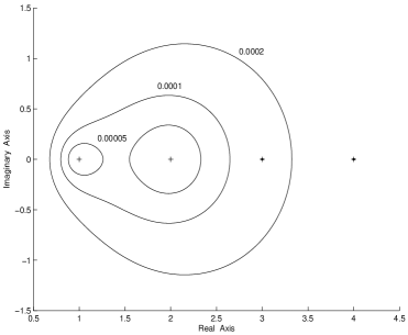
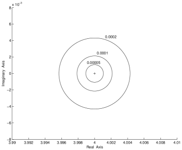
Refer to caption Refer to caption

Figure 2: The boundaries σε(P)subscript𝜎𝜀𝑃\,\partial\sigma_{\varepsilon}(P)\, for ε=5105,104,2104𝜀5superscript105superscript1042superscript104\,\varepsilon=5\cdot 10^{-5},10^{-4},2\cdot 10^{-4}.

The left part of Figure 2 indicates the boundaries of the pseudospectra σε(P)subscript𝜎𝜀𝑃{\sigma}_{\varepsilon}(P) for ε=5105,104,2104𝜀5superscript105superscript1042superscript104\,\varepsilon=5\cdot 10^{-5},10^{-4},2\cdot 10^{-4}. The eigenvalues of P(λ)𝑃𝜆P({\lambda}) are marked with ++’s. The small components of σ5105(P)subscript𝜎5superscript105𝑃\,{\sigma}_{5\cdot 10^{-5}}(P), σ104(P)subscript𝜎superscript104𝑃{\sigma}_{10^{-4}}(P)\, and σ2104(P)subscript𝜎2superscript104𝑃\,{\sigma}_{2\cdot 10^{-4}}(P)\, that correspond to the eigenvalue λ=4𝜆4{\lambda}=4 are not visible in the left part of the figure, and they are magnified in the right part. Note that these components almost coincide with circular discs centered at λ=4𝜆4{\lambda}=4 of radii k(P,4)ε𝑘𝑃4𝜀\,k(P,4)\,\varepsilon, ε=5105,104,2104𝜀5superscript105superscript1042superscript104\,\varepsilon=5\cdot 10^{-5},10^{-4},2\cdot 10^{-4}, as expected from Proposition 1. It is also apparently confirmed that the eigenvalue λ=2𝜆2{\lambda}=2 is more sensitive than the eigenvalue λ=1𝜆1{\lambda}=1 (more particularly, one may say that the eigenvalue λ=2𝜆2{\lambda}=2 is more than twice as sensitive as λ=1𝜆1{\lambda}=1), and that both of them are much more sensitive than the eigenvalue λ=4𝜆4{\lambda}=4.

6 An Elsner-like bound

In this section, we apply the Elsner technique [8] (see also [22]) to obtain a perturbation result for matrix polynomials. This technique allows large perturbations, yielding error bounds, and it does not distinguish between ill-conditioned and well-conditioned eigenvalues.

Theorem 10.

Consider a matrix polynomial P(λ)𝑃𝜆P({\lambda}) as in (1) and a perturbation Q(λ)(P,ε,w)𝑄𝜆𝑃𝜀wQ({\lambda})\in{\mathcal{B}}(P,\varepsilon,\textup{w}) as in (3). For any μσ(Q)\σ(P),𝜇\𝜎𝑄𝜎𝑃\,\mu\in{\sigma}(Q)\backslash{\sigma}(P),\, it holds that

minλσ(P)|μλ|(εw(|μ|)|detAm|)1mnP(μ)11mn.subscript𝜆𝜎𝑃𝜇𝜆superscript𝜀𝑤𝜇subscript𝐴𝑚1𝑚𝑛superscriptnorm𝑃𝜇11𝑚𝑛\min_{{\lambda}\in{\sigma}(P)}|\mu-{\lambda}|\,\leq\,\left(\frac{\varepsilon\,w(|\mu|)}{|\det A_{m}|}\right)^{\frac{1}{mn}}\left\|P(\mu)\right\|^{1-\frac{1}{mn}}.
Proof.

Let σ(P)={λ1,λ2,,λnm},𝜎𝑃subscript𝜆1subscript𝜆2subscript𝜆𝑛𝑚\,{\sigma}(P)=\{{\lambda}_{1},{\lambda}_{2},\dots,{\lambda}_{nm}\},\, counting algebraic multiplicities, and suppose μσ(Q)\σ(P)𝜇\𝜎𝑄𝜎𝑃\mu\in{\sigma}(Q)\backslash{\sigma}(P). Then

minλσ(P)|μλ|nmi=1nm|μλi|=|detP(μ)||detAm|.subscript𝜆𝜎𝑃superscript𝜇𝜆𝑛𝑚superscriptsubscriptproduct𝑖1𝑛𝑚𝜇subscript𝜆𝑖𝑃𝜇subscript𝐴𝑚\min_{{\lambda}\in{\sigma}(P)}\left|\mu-{\lambda}\right|^{nm}\,\leq\,\prod_{i=1}^{nm}|\mu-{\lambda}_{i}|\,=\,\frac{|\det P(\mu)|}{|\det A_{m}|}.

Let now U=[u1u2un]𝑈delimited-[]subscript𝑢1subscript𝑢2subscript𝑢𝑛U=\left[\,u_{1}\;\,u_{2}\;\cdots\;u_{n}\,\right] be an n×n𝑛𝑛n\times n unitary matrix such that Q(μ)u1=0𝑄𝜇subscript𝑢10Q(\mu)u_{1}=0. By Hadamard’s inequality [22] (see also [23, Theorem 2.4]), it follows

minλσ(P)|μλ|nmsubscript𝜆𝜎𝑃superscript𝜇𝜆𝑛𝑚\displaystyle\min_{{\lambda}\in{\sigma}(P)}\left|\mu-{\lambda}\right|^{nm} \displaystyle\leq |detP(μ)||detAm|=|detP(μ)||detU||detAm|𝑃𝜇subscript𝐴𝑚𝑃𝜇𝑈subscript𝐴𝑚\displaystyle\frac{|\det P(\mu)|}{|\det A_{m}|}\,=\,\frac{|\det P(\mu)|\,\,|\det U|}{|\det A_{m}|}
\displaystyle\leq 1|detAm|i=1nmP(μ)ui1subscript𝐴𝑚superscriptsubscriptproduct𝑖1𝑛𝑚norm𝑃𝜇subscript𝑢𝑖\displaystyle\frac{1}{|\det A_{m}|}\,\,\prod_{i=1}^{nm}\left\|P(\mu)u_{i}\right\|
=\displaystyle= 1|detAm|P(μ)u1i=2nmP(μ)ui1subscript𝐴𝑚norm𝑃𝜇subscript𝑢1superscriptsubscriptproduct𝑖2𝑛𝑚norm𝑃𝜇subscript𝑢𝑖\displaystyle\frac{1}{|\det A_{m}|}\left\|P(\mu)u_{1}\right\|\prod_{i=2}^{nm}\left\|P(\mu)u_{i}\right\|
=\displaystyle= 1|detAm|P(μ)u1Q(μ)u1i=2nmP(μ)ui1subscript𝐴𝑚norm𝑃𝜇subscript𝑢1𝑄𝜇subscript𝑢1superscriptsubscriptproduct𝑖2𝑛𝑚norm𝑃𝜇subscript𝑢𝑖\displaystyle\frac{1}{|\det A_{m}|}\left\|P(\mu)u_{1}-Q(\mu)u_{1}\right\|\,\,\prod_{i=2}^{nm}\left\|P(\mu)u_{i}\right\|
\displaystyle\leq 1|detAm|Δ(μ)u1P(μ)nm11subscript𝐴𝑚normΔ𝜇subscript𝑢1superscriptnorm𝑃𝜇𝑛𝑚1\displaystyle\frac{1}{|\det A_{m}|}\left\|{\Delta}(\mu)u_{1}\right\|\left\|P(\mu)\right\|^{nm-1}
\displaystyle\leq εw(|μ|)|detAm|P(μ)nm1,𝜀𝑤𝜇subscript𝐴𝑚superscriptnorm𝑃𝜇𝑛𝑚1\displaystyle\frac{\varepsilon\,\,w(|\mu|)}{|\det A_{m}|}\left\|P(\mu)\right\|^{nm-1},

and the proof is complete. ∎

Recently, the classical Bauer-Fike Theorem [3] has been generalized to the case of matrix polynomials [6]. Applying the arguments of the proof of Theorem 4.1 in [6], it is easy to verify the “weighted version” of the result.

Theorem 11.

Consider a matrix polynomial P(λ)𝑃𝜆P({\lambda}) as in (1) and a perturbation Q(λ)(P,ε,w)𝑄𝜆𝑃𝜀wQ({\lambda})\in{\mathcal{B}}(P,\varepsilon,\textup{w}) as in (3), and let (X,J,Y)𝑋𝐽𝑌(X,J,Y) be a Jordan triple of P(λ)𝑃𝜆P({\lambda}). For any μσ(Q)\σ(P)𝜇\𝜎𝑄𝜎𝑃\mu\in{\sigma}(Q)\backslash{\sigma}(P), it holds that minλσ(P)|μλ|max{ϑ,ϑ1/p},subscript𝜆𝜎𝑃𝜇𝜆italic-ϑsuperscriptitalic-ϑ1𝑝\,\min\limits_{{\lambda}\in{\sigma}(P)}|\mu-{\lambda}|\leq\max\left\{\vartheta,\,\vartheta^{1/p}\right\},\, where ϑ=pk(P)εw(|μ|)italic-ϑ𝑝𝑘𝑃𝜀𝑤𝜇\,\vartheta=p\ k(P)\,\varepsilon\,w(|\mu|)\, and p𝑝\,p\, is the maximum dimension of the Jordan blocks of J𝐽J.

To compare these two bounds, we consider the matrix polynomial

P(λ)=Iλ3+[0220]λ2+[0110]λ𝑃𝜆𝐼superscript𝜆3delimited-[]0220superscript𝜆2delimited-[]0110𝜆P({\lambda})\,=\,I{\lambda}^{3}+\left[\begin{array}[]{cc}0&\sqrt{2}\\ \sqrt{2}&0\end{array}\right]{\lambda}^{2}+\left[\begin{array}[]{cc}0&-1\\ 1&0\end{array}\right]{\lambda}

(see [6, Example 1] and [10, Example 1.5]) with detP(λ)=λ2(λ+1)2(λ1)2𝑃𝜆superscript𝜆2superscript𝜆12superscript𝜆12\,\det P({\lambda})={\lambda}^{2}({\lambda}+1)^{2}({\lambda}-1)^{2}. A Jordan triple (X,J,Y)𝑋𝐽𝑌(X,J,Y) of P(λ)𝑃𝜆P({\lambda}) is given by

X=[102+1222+12+2011010],J=[000000000000001100000100000011000001]formulae-sequence𝑋delimited-[]1021222122011010𝐽delimited-[]000000000000001100000100000011000001X=\left[\begin{array}[]{cccccc}1&0&-\sqrt{2}+1&\sqrt{2}-2&\sqrt{2}+1&\sqrt{2}+2\\ 0&1&1&0&1&0\end{array}\right],\,\,J=\left[\begin{array}[]{cccccc}0&0&0&0&0&0\\ 0&0&0&0&0&0\\ 0&0&1&1&0&0\\ 0&0&0&1&0&0\\ 0&0&0&0&-1&1\\ 0&0&0&0&0&-1\end{array}\right]
andYT=14[042+2212+22+1400101].andsuperscript𝑌𝑇14delimited-[]0422212221400101\mbox{and}\;\;\;Y^{T}=\,\frac{1}{4}\left[\begin{array}[]{cccccc}0&-4&\sqrt{2}+2&-\sqrt{2}-1&-\sqrt{2}+2&-\sqrt{2}+1\\ 4&0&0&1&0&-1\end{array}\right].

The associated condition number of the eigenproblem of P(λ)𝑃𝜆P({\lambda}) is k(P)=6.4183𝑘𝑃6.4183\,k(P)=6.4183. For ε=0.3𝜀0.3\varepsilon=0.3 and w={w0,w1,w2,w3}={0.1,1,1,0}wsubscript𝑤0subscript𝑤1subscript𝑤2subscript𝑤30.1110\textup{w}=\{w_{0},w_{1},w_{2},w_{3}\}=\{0.1,1,1,0\}, the matrix polynomial

Q(λ)=Iλ3+[i 0.322i 0.3]λ2+[00.70.70]λ+[0.01000.03]𝑄𝜆𝐼superscript𝜆3delimited-[]i0.322i0.3superscript𝜆2delimited-[]00.70.70𝜆delimited-[]0.01000.03Q({\lambda})\,=\,I{\lambda}^{3}+\left[\begin{array}[]{cc}\textup{i}\,0.3&\sqrt{2}\\ \sqrt{2}&-\textup{i}\,0.3\end{array}\right]{\lambda}^{2}+\left[\begin{array}[]{cc}0&-0.7\\ 0.7&0\end{array}\right]{\lambda}+\left[\begin{array}[]{cc}0.01&0\\ 0&0.03\end{array}\right]

lies on the boundary of (P,0.3,w)𝑃0.3w\mathcal{B}\left(P,0.3,\textup{w}\right) and has μ=0.5691+i 0.0043𝜇0.5691i0.0043\mu=0.5691+\textup{i}\,0.0043 as an eigenvalue. Then minλσ(P)|μλ|=|0.5691+i 0.00431|=0.4309,subscript𝜆𝜎𝑃𝜇𝜆0.5691i0.004310.4309\,\min\limits_{{\lambda}\in{\sigma}(P)}\left|\mu-{\lambda}\right|=|0.5691+\textup{i}\,0.0043-1|=0.4309,\, the upper bound of Theorem 10 is  0.8554,0.8554\,0.8554,\, and the upper bound of Theorem 11 is  3.82403.8240\,3.8240.

It is clear that the Elsner-like upper bound is tighter than the upper bound of Theorem 11 when P(μ)norm𝑃𝜇\|P(\mu)\| is sufficiently small; this is the case in the above example, where P(0.5691+i 0.0043)=1.0562norm𝑃0.5691i0.00431.0562\|P(0.5691+\textup{i}\,0.0043)\|=1.0562. In particular, if we define the quantity

Ω(P,ε,μ)={|detAm|(pk(P))mn(εw(|μ|))mn1,whenpk(P)εw(|μ|)1|detAm|(pk(P))mnp(εw(|μ|))mnp1,whenpk(P)εw(|μ|)<1,Ω𝑃𝜀𝜇casessubscript𝐴𝑚superscript𝑝𝑘𝑃𝑚𝑛superscript𝜀𝑤𝜇𝑚𝑛1when𝑝𝑘𝑃𝜀𝑤𝜇1subscript𝐴𝑚superscript𝑝𝑘𝑃𝑚𝑛𝑝superscript𝜀𝑤𝜇𝑚𝑛𝑝1when𝑝𝑘𝑃𝜀𝑤𝜇1\Omega(P,\varepsilon,\mu)\,=\,\left\{\begin{array}[]{l}|\det A_{m}|\ (p\ k(P))^{mn}\,(\varepsilon\,w(|\mu|))^{mn-1},\;\mbox{when}\;\;p\ k(P)\,\varepsilon\,w(|\mu|)\geq 1\\ |\det A_{m}|\ (p\ k(P))^{\frac{mn}{p}}\,(\varepsilon\,w(|\mu|))^{\frac{mn}{p}-1},\;\mbox{when}\;\;p\ k(P)\,\varepsilon\,w(|\mu|)<1\end{array}\right.,

then it is straightforward to see that the bound of Theorem 10 is better than the bound of Theorem 11 if and only if P(μ)<Ω(P,ε,μ)1mn1norm𝑃𝜇Ωsuperscript𝑃𝜀𝜇1𝑚𝑛1\;\|P(\mu)\|\,<\,\Omega(P,\varepsilon,\mu)^{\frac{1}{mn-1}}.

References

  • [1]
  • [2] A.L. Andrew, K.-W.E. Chu and P. Lancaster, Derivatives of eigenvalues and eigenvectors of matrix functions, SIAM J. Matrix Anal. Appl., 14 (1993) 903–926.
  • [3] F.L. Bauer and C.T. Fike, Norms and exclusion theorems, Numer. Math., 2 (1960) 137–144.
  • [4] L. Boulton, P. Lancaster and P. Psarrakos, On pseudospecta of matrix polynomials and their boundaries, Math. Comp., 77 (2008) 313–334.
  • [5] J.V. Burke, A.S. Lewis and M.L. Overton, Spectral conditioning and pseudospectral growth, Numer. Math., 107 (2007) 27–37.
  • [6] K.-W.E. Chu, Perturbation of eigenvalues for matrix polynomials via the Bauer-Fike theorems, SIAM J. Matrix Anal. Appl., 25 (2003) 551–573.
  • [7] J.W. Demmel, On condition numbers and the distance to the nearest ill-posed problem, Numer. Math., 51 (1987) 251–289.
  • [8] L. Elsner, An optimal bound for the spectral variation of two matrices, Linear Algebra Appl., 71 (1985) 77–80.
  • [9] M. Embree and L.N. Trefethen, Spectra and Pseudospectra: The Behavior of Nonnormal Matrices and Operators, Princeton University Press, 2005.
  • [10] I. Gohberg, P. Lancaster and L. Rodman, Matrix Polynomials, Academic Press, New York, 1982.
  • [11] M. Karow, Geometry of Spectral Valued Sets, PhD Thesis, University of Bremen, 2003.
  • [12] D. Kressner, M.J. Peláez and J. Moro, Structured Hölder condition numbers for multiple eigenvalues, preprint, 2008.
  • [13] P. Lancaster and P. Psarrakos, On the pseudospectra of matrix polynomials, SIAM J. Matrix Anal. Appl., 27 (2005) 115–129.
  • [14] P. Lancaster and M. Tismenetsky, The Theory of Matrices, 2nd edition, Academic Press, Orlando, 1985.
  • [15] D.S. Mackey, Structured Linearizations for Matrix Polynomials, PhD Thesis, University of Manchester, 2006.
  • [16] A.S. Markus, Introduction to the Spectral Theory of Polynomial Operator Pencils, Amer. Math. Society, Providence, Translations of Math. Monographs, Vol. 71, 1988.
  • [17] J. Moro, J.V. Burke and M.L. Overton, On the Lidskii-Vishik-Lyusternik perturbation theory for eigenvalues of matrices with arbitrary Jordan structure, SIAM J. Matrix Anal. Appl., 18 (1997) 793–817.
  • [18] N. Papathanasiou and P. Psarrakos, The distance from a matrix polynomial to matrix polynomials with a prescribed multiple eigenvalue, Linear Algebra Appl., 429 (2008) 1453–1477.
  • [19] A. Ruhe, Properties of a matrix with a very ill-conditioned eigenprolem, Numer. Math., 15 (1970) 57–60.
  • [20] R.A. Smith, The condition numbers of the matrix eigenvalue problem, Numer. Math., 10 (1967) 232–240.
  • [21] G.W. Stewart, Error bounds for approximate invariant subspaces of closed linear operators, SIAM J. Numer. Anal., 8 (1971) 796–808.
  • [22] G.W. Stewart, An Elsner-like perturbation theorem for generalized eigenvalues, Linear Algebra Appl., 390 (2004) 1–5.
  • [23] G.W. Stewart and J.-G. Sun, Matrix Perturbation Theory, Academic Press, New York, 1990.
  • [24] F. Tisseur, Backward error and condition of polynomial eigenvalue problems, Linear Algebra Appl., 309 (2000) 339–361.
  • [25] F. Tisseur and N.J. Higham, Structured pseudospectra for polynomial eigenvalue problems with applications, SIAM J. Matrix Anal. Appl., 23 (2001) 187–208.
  • [26] J.H. Wilkinson, The Algebraic Eigenvalue Problem, Claredon Press, Oxford, 1965.
  • [27] J.H. Wilkinson, Note on matrices with a very ill-conditioned eigenprolem, Numer. Math., 19 (1972) 175–178.
  • [28] J.H. Wilkinson, On neighbouring matrices with quadratic elementary divisors, Numer. Math., 44 (1984) 1–21.
  • [29]