Random copolymer adsorption: Morita approximation compared to exact numerical simulations

Abstract

We study the adsorption of ideal random lattice copolymers with correlations in the sequences on homogeneous substrates with two different methods: An analytical solution of the problem based on the constrained annealed approximation introduced by Morita in 1964 and the generating functional (GF) technique, and direct numerical simulations of lattice chains averaged over many realizations of random sequences. Both methods allow to calculate the free energy and different conformational characteristics of the adsorbed chain. The comparison of the results for random copolymers with different degree of correlations and different types of nonadsorbing monomers (neutral or repelling from the surface) shows not only qualitative but a very good quantitative agreement, especially in the cases of Bernoullian and quasi-alternating random sequences.

I Introduction

Random copolymers (RC) attract much attention and have been studied intensively in the last two decades. This is motivated, on the one hand, by the nontrivial properties of individual RCs and their behaviour in solutions and melts, and, on the other hand, by the biological relevance of this class of molecules (protein Pande:2000 and RNA Bundschuh:2002 folding, hybridisation of heterogeneous DNA Garel:2005 , because real proteins and nucleic acids represent, with no doubt, irregular copolymers.

Among the many open questions involving RCs, the problem of RC adsorption at different interfaces is taking a particularly prominent place, because of the technological relevance of such systems, their role as biomimetic model systems for molecular recognition Chakraborty:2001 etc.), and the basic challenges they offer for theoretical physicists and applied mathematicians. Several types of interfaces have been considered, interfaces that are penetrable for polymer such as liquid/liquid interfaces or lipid membranes, and impenetrable solid substrates, either with or without chemical or geometrical homogeneities Sommer:1995 ; Trovato:1999 ; Chen:2000 ; Denesyuk:2000 ; Polotsky:2004a ; Polotsky:2004b ; Orlandini:2002 ; Iliev:2004 ; Alvarez:2007 . In the present paper we focus on the problem of adsorption of a single ideal RC chain with correlations in the monomer sequence on an impenetrable planar surface using a lattice model.

Solving problems that involve RCs, one faces the necessity to carry out two operations: Firstly, one needs to sum over the statistical weights of polymer conformations, i.e. to calculate the system’s partition function $Z$ and the free energy $F$ (the logarithm of the partition function, $F=-k_{B}T\log Z$), and secondly, one needs to average the free energy with respect to the disorder in the RC monomer sequence. Averaging “$\log Z$” over the sequence disorder turns out to be a very difficult task which can seldom be carried out rigorously. It would be much easier to average the partition function prior to taking its logarithm, but this corresponds to the physically different situation of annealed disorder (in our system the monomer sequence is quenched), which approximates the quenched situation only very poorly. One common approach consists in using the replica trick which then can be combined with some variational scheme (e.g., the reference system approach suggested by Chen Chen:2000 ; Denesyuk:2000 ; Polotsky:2004a ; Polotsky:2004b , or the Gaussian variational approach Trovato:1999 ).

In the present work, we exploit another approximation to resolve the difficulties with the quenched average - the constrained annealing suggested by T. Morita in 1964 Morita:1964 . In this approximation scheme, one averages over annealed disorder (i.e. directly averages the partition function), but imposes the constraint that the first, the second, etc., moments of the monomer distribution in the RC sequence keep their correct values. The ideas of the method are developed in the original paper of Morita Morita:1964 ; a more detailed and formalized description can be found in the paper of Kühn Kuehn:1996 and in a recent review of Soteros and Whittington Soteros:2004 .

For the problem of RC adsorption on the solid interface and RC localization at the liquid-liquid interface, the Morita approximation has been successfully applied by Whittington and Orlandini et al. Orlandini:2002 ; Iliev:2004 . In these works, the authors considered simplified polymer models - fully directed random walks in 2D space (Dyck and Motzkin paths). RC localization at penetrable and impenetrable interfaces Orlandini:2002 (with both chain ends fixed at the interface) as well as the adsorption-desorption transition upon pulling one chain end away from the interface by an external force Iliev:2004 were studied. The Morita approximation was first order, i.e., only a constraint on the first moment of the monomer distribution was imposed. (Note that the annealed approximation can formally be considered as a zero order Morita approximation.)

Higher order Morita approximations were applied to the RC adsorption problem by Alvarez et al. Alvarez:2007 , where polymer trajectories were again modeled by Dyck and Motzkin paths. The authors obtained lower bounds limiting the quenched free energy and demonstrated how these bounds improve as the order of the Morita approximation increases. In contrast, the location of the phase boundary is not more accurate in the Morita approximation than in the annealed approximation, as was rigorously proved by Caravenna and Giacomin Caravenna:2005

The simplified polymer models (Dyck and Motzkin paths) considered in the previous works Orlandini:2002 ; Iliev:2004 ; Alvarez:2007 have their doubtless advantages of being exactly solvable and at the same time permitting to obtain a physically clear and tractable picture of the studied phenomena. However, real polymers “live” in the 3-dimensional space and are not necessarily directed. Furthermore, the RCs in Refs. Orlandini:2002, ; Iliev:2004, ; Alvarez:2007, were of Bernoullian type, i.e., uncorrelated. In the present paper we study – although somewhat simplified – a 3-dimensional situation and a wider class of RCs with correlations in the monomer sequence, where Bernoullian RCs represent one special case.

The calculation of the partition function via summation over polymer conformations is carried out using the generating function (GF) approach (or grand canonical approach) developed for polymeric systems by Lifson Lifson:1964 . This very general method has been used to study conformational transitions in polypeptides (coil – $\alpha$-helix Poland:1965 and coil – $\beta$-structure Birshtein:1971 ) and DNA (coil – double helix) Litan:1965 ; Poland:1966 . Birshtein was the first to apply it to the problem of single polymer adsorption Birshtein:1979 ; Birshtein:1983 . She developed a theory of the adsorption transition based on the GF formalism and demonstrated its power and generality with a number of different examples. The approach allowed to reproduce very elegantly a number of previously known results, and, in the same easy manner, to treat the more complicated case when adsorption is coupled with a helix-coil transition in the chain. In her work Birshtein Birshtein:1979 ; Birshtein:1983 focused on the adsorption-desorption transition point and the order of the transition. Later, the results of her theory were used to analyze the adsorption-desorption transition for regular $\mathrm{\left(A_{m}B_{n}\right)_{x}}$-multiblock copolymers Zhulina:1981 . Brun Brun:1999 has proposed an approximate generalization of the equation for the transition point in Ref. Birshtein:1979, for correlated annealed RCs (see section III.1).

The method of GF is highly general and its success is due to the possibility to calculate the GF for elements of the chain conformations. Despite the fact that it is more than 30 years old, it is still often used up to date. One of the most prominent examples is the ongoing discussion about the order of the DNA denaturation transition Kafri:2000 ; Kafri:2002 ; Garel:2001 ; Richard:2004 , which is carried on - for the most part - in the framework of this approach. We also note that in its “continuous” version, the method of GF is equivalent to the propagator formalism in Fourier-Laplace space – see, for instance, Muthukumar et al. Muthukumar:1996 ; Carri:1999 .

In the present work, analytical calculations based on the Morita approximation and the GF approach (though the final equations can only be solved numerically, the disorder average and the summation over chain conformations are carried out analytically) are supplemented with numerical simulations for tethered RC chains. In the simulations, a sample of several (sufficiently many) RC sequences are drawn randomly from the desired distribution. For each chain, the propagators are calculated exactly (recursively). This allows to evaluate the free energy and different observables directly and carry out an “exact” quenched average over the sequence disorder. The comparison of the results obtained with the two different methods allows us to make a conclusion about the accuracy and applicability of the Morita approximation.

The rest of the paper is organized as follows. Section II defines the model and introduces the annealed and the Morita approximation. Although the annealed approximation is deficient in many respect, it is convenient to introduce the GF approach in this framework. This is done in Section II.3. An additional motivation for treating the annealed case in detail is that there is a class of so called two-state or annealed copolymers, which are adequately described by the annealed approximation (see Ref. [Yoshinaga:2008, ] and references therein). The generalisation to the Morita approximation in Section II.3 is quite simple and transparent. In Section II.4 our numerical approach is introduced. The results obtained using both methods are compared and discussed in Section III. Finally, Section IV presents the summary and final conclusions.

II Model and method

II.1 Definition of the model

Consider a RC chain consisting of $N$ monomer units near an impenetrable surface, Fig. 1. A lattice model of the polymer is employed, i.e. each chain conformation is represented as a walk on the lattice. Monomer units in the RC chain can either be of type A or of type B, and their sequence is taken to be random. We assume that there are no excluded-volume interactions between monomers (i.e., we consider the case of ideal chains), but there is a short-range interaction between monomers and the surface. The Hamiltonian of the system can be written as

$$H=\sum_{i=1}^{N}\Delta_{i}\cdot\left[\chi_{i}\varepsilon_{A}+(1-\chi_{i})\varepsilon_{B}\right].$$ (1)

Here $\chi_{i}$ indicates the type of the monomer $i$:

$$\chi_{i}=\left\{\begin{array}[]{ll}1&\mbox{for A-monomer }\left(\mbox{giving }[...]=\varepsilon_{A}\right)\\ 0&\mbox{for B-monomer }\left(\mbox{giving }[...]=\varepsilon_{B}\right)\end{array}\right.$$ (2)

and $\Delta_{i}$ is a conformation-dependent parameter, namely, $\Delta_{i}=1$ if $i$-th monomer occupies a site adjacent to the adsorbing surface and 0 otherwise. Any contact of an A monomer with the surface leads to an energy contribution $\varepsilon_{A}$, and likewise, a contact of a B monomer contributes $\varepsilon_{B}$.

Figure 1: Random copolymer near adsorbing plane.

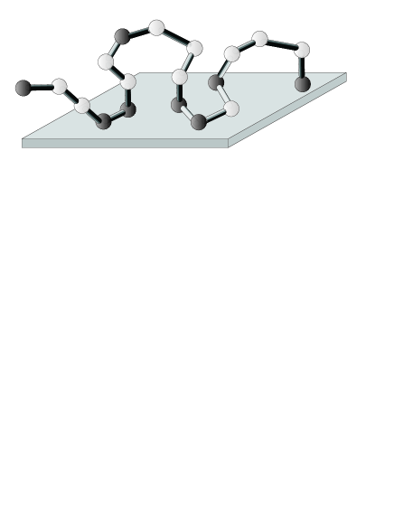
The monomer sequence $\chi=\{\chi_{1},\chi_{2},...,\chi_{N}\}$ is random and will be represented as a first order Markov chain. It is determined by the probabilities to find A and B monomers in the sequence

$$P(\chi_{i}=A)=f_{A}\,\mbox{ and }\,P(\chi_{i}=B)=f_{B}=1-f_{A}$$ (3)

and by the probabilities that the monomer of the type $i$ is followed by the monomer of the type $j$, $P(\chi_{m}=j|\chi_{m-1}=i)=p_{ij}$

$$\mathbf{P}=\left(\begin{array}[]{cc}p_{AA}&p_{AB}\\ p_{BA}&p_{BB}\end{array}\right)=\left(\begin{array}[]{cc}p_{AA}&1-p_{AA}\\ 1-p_{BB}&p_{BB}\end{array}\right).$$ (4)

The transition probabilities are normalized : $\sum_{j}p_{ij}=1$. We also assume that the Markov chain is reversible, i.e. $f_{i}p_{ij}=f_{j}p_{ji}$. Hence,the probability of the sequence $\chi=\{\chi_{1},\chi_{2},...,\chi_{N}\}$ to appear is given by the product

$$P(\chi)\equiv P(\chi_{1},\chi_{2},\ldots,\chi_{n})=f_{\chi_{1}}\cdot p_{\chi_{1}\chi_{2}}\cdot p_{\chi_{2}\chi_{3}}\cdot\ldots\cdot p_{\chi_{n-1},\,\chi_{n}}.$$ (5)

It is convenient to introduce the cluster parameter $c$:

$$c:=1-p_{AB}-p_{BA}=p_{AA}+p_{BB}-1,$$ (6)

which characterizes the correlations in the sequence: $c>0$ means that there is a tendency in the sequence for grouping similar monomers into clusters, $c<0$ favors the alternating sequence of A’s and B’s, $c=0$ corresponds to uncorrelated (Bernoullian) sequences. The cases $c=-1$ is also special, since it describes perfectly ordered alternating block copolymers ($...ABABAB...$).

Because of the normalization and reversibility conditions, it is sufficient to prescribe any two of these parameters to completely determine the first order Markov chain, for example, $f_{A}$ and $c$. Then

$$\begin{array}[]{ll}p_{AA}=f_{A}+c(1-f_{A})\,,&p_{AB}=(1-f_{A})(1-c)\\ p_{BA}=f_{A}(1-c)\,,&p_{BB}=1-f_{A}+cf_{A}.\end{array}$$ (7)

Finally, it should be noted that the range of possible values for $f_{A}$ depends on the value of $c$: for $c\geq 0$ $f_{A}$ may take any value between 0 and 1 whereas for $c<0$ there is a constraint

$$-\frac{c}{1-c}<f_{A}<\frac{1}{1-c}\,.$$ (8)

In the actual calculations of this paper, we consider two cases:

• A monomer is attracted by the surface ($\varepsilon_{A}=-1$), B monomer is neutral ($\varepsilon_{B}=0$), denoted as SN (sticky-neutral) case

• A monomer is attracted by the surface ($\varepsilon_{A}=-1$), B monomer is repelled from the surface ($\varepsilon_{B}=1$), denoted as SR (sticky-repulsive) case

It should be emphasized that the terms “neutral” or “repulsive” are applied to monomer-surface interaction whereas a polymer chain composed of either neutral or repulsive monomers will effectively repel from the surface.

II.2 Disorder average and Morita approximation

Having introduced the model, let us now write the system’s partition function for a given realization of the monomer sequence

$$Z_{N}(\beta|\chi)=\sum_{\omega}\exp\left\{-\beta\sum_{i=1}^{N}\Delta_{i}\cdot\left[\chi_{i}\varepsilon_{A}+(1-\chi_{i})\varepsilon_{B}\right]\right\},$$ (9)

where $\beta$ is the inverse temperature and $\sum_{\omega}$ denotes the sum over all chain conformations $\omega$.

Rather than dealing with particular realizations of a RC sequence, we study the whole ensemble of RC chains with the desired statistics. The randomness in the RC sequence is quenched, which means that after synthesis of a RC chain, its monomer sequence remains unchanged. To obtain the quenched free energy, the logarithm of the partition function should be averaged over all possible sequence realizations:

$$\beta F_{q}=-\left\langle\log Z_{N}(\beta|\chi)\right\rangle$$ (10)

where the angular brackets $\left\langle\ldots\right\rangle$ denote averaging over sequence randomness

$$\left\langle A\right\rangle:=\sum_{\chi}P(\chi)A(\chi).$$ (11)

Direct averaging of the $\log Z_{N}$ is, in general, a rather difficult problem, so one can use, for example, the replica trick and work formally with an $m$ times replicated system Soteros:2004 ; Chen:2000 ; Stepanow:2002 ; Polotsky:2004a ; Polotsky:2004b .

Averaging of the partition function prior to taking the logarithm corresponds to the annealed type of disorder. In this case, the average is evaluated according to

$$\beta F_{a}=-\log\left\langle Z_{N}(\beta|\chi)\right\rangle,$$ (12)

where

$$\left\langle Z_{N}(\beta|\chi)\right\rangle=\sum_{\chi}P(\chi)\sum_{\omega}\exp\left\{-\beta\sum_{i=1}^{N}\Delta_{i}\cdot\left[\chi_{i}\varepsilon_{A}+(1-\chi_{i})\varepsilon_{B}\right]\right\}.$$ (13)

Physically, annealed disorder means that the type of any monomer (and its affinity to the surface, in our case) may change while the system attains its equilibrium state Yoshinaga:2008 . The annealed approximation can roughly be considered as the “zero order” approach to the problem of carrying out a quenched average. It is substantially easier to perform but it often fails to give good values for the free energy and other observables. The annealed approximation does not guarantee that even the lower moments of the distribution of monomers remain correct in the final result.

To approach this problem, Morita Morita:1964 has suggested to use a partial annealing procedure where the moments of the monomer distribution are constrained to keep their correct values. For example, in our case, the constraint on the first moment reads

$$\frac{1}{N}\sum_{i=1}^{N}\chi_{i}=f_{A},$$ (14)

the second moment of the distribution is constrained according to

$$\frac{1}{N-1}\sum_{i=2}^{N}\chi_{i-1}\chi_{i}=f_{AA},$$ (15)

where $f_{AA}=f_{A}\cdot p_{AA}$ is the AA dyad probability, and so on. For the averaging of the partition function, this means that we introduce the constraints (14)-(15) into Eq. (13) via Lagrange multipliers $\lambda$ and $\kappa$:

$$\begin{split}\left\langle Z_{N}(\beta|\chi)\right\rangle_{M}=&\sum_{\chi}P(\chi)\sum_{\omega}\exp\left\{-\beta\sum_{i=1}^{n}\Delta_{i}\cdot\left[\chi_{i}\varepsilon_{A}+(1-\chi_{i})\varepsilon_{B}\right]\right\}\\ \times&\,\exp\left\{\lambda\left(\sum_{i=1}^{N}\chi_{i}-Nf_{A}\right)+\kappa\left(\sum_{i=2}^{N}\chi_{i-1}\chi_{i}-(N-1)f_{AA}\right)\right\}.\end{split}$$ (16)

and request

$$\begin{split}&\frac{\partial\log\left\langle Z_{N}(\beta|\chi)\right\rangle_{M}}{\partial\lambda}=\left\langle\sum_{i=1}^{N}\chi_{i}\right\rangle-Nf_{A}=0,\\ &\frac{\partial\log\left\langle Z_{N}(\beta|\chi)\right\rangle_{M}}{\partial\kappa}=\left\langle\sum_{i=2}^{N}\chi_{i-1}\chi_{i}\right\rangle-(N-1)f_{AA}=0\,.\end{split}$$ (17)

Here and below the notation $\left\langle\ldots\right\rangle_{M}$ for the disorder average subjected to the Morita conditions is used. After exchanging the order of conformational and disorder average (i.e. the order of summation $\sum_{\chi}\sum_{\omega}=\sum_{\omega}\sum_{\chi}$), the partition function reduces to the sum of the pre-averaged statistical (Boltzmann) weights over polymer conformations. In the present work this sum is calculated using the GF approach (or grand canonical approach) developed for linear polymers by Lifson Lifson:1964 .

II.3 Sum over conformation and GF approach

The main object (concept) of the GF approach is the GF

$$\Gamma(x)=\sum_{N=1}^{\infty}Z_{N}x^{N}\,,$$ (18)

where $Z_{N}$ is the partition function of a polymer chain with $N$ units. The GF can be considered as the grand canonical partition function; in this case, $x\equiv\exp(\mu/k_{B}T)$, where $\mu$ is the chemical potential of a monomer unit and $x$ is called monomer activity. Once the GF (18) is known, the partition function $Z_{N}$ can be formally determined as the coefficients of the expansion of $\Gamma(x)$ in powers of $x$. In the long chain limit, $N\gg 1$, the asymptotic expression for $Z_{N}$ is even simpler since it is dominated by the smallest singularity $x_{c}$ of $\Gamma(x)$: $Z_{N}\simeq x_{c}^{-N}$.

The GF approach is particularly efficient in the cases where monomer unit may exist in one of several states (for example, double helical or coil in DNA Litan:1965 ; Poland:1966 , $\alpha$-helical and coil Poland:1965 or $\beta$-structure and coil Birshtein:1971 in polypeptides) and the chain conformation can be represented as an alternation (not necessary regular) of sequences of different types.

To study RC adsorption, we generalize the work of Birshtein, who was the first to apply the GF formalism to the problem of homopolymer adsorption Birshtein:1979 ; Birshtein:1983 . For clarity, we first illustrate our approach for the case of annealed RCs.

For an adsorbed chain, each adsorbed conformation can be represented as a sequence of adsorbed and desorbed groups of monomers. The adsorbed sequences are called trains, among the desorbed we distinguish between tails at the ends of the chain and loops separating adsorbed sequences. It is clear that an adsorbed chain can have at most two tails, $n_{T}\leq 2$, whereas the number of loops is less than the number of trains by unity, i.e. if $n_{L}=n_{S}-1$. We note that different tails, loops, and trains do not interact with each other. The GF of the partition function, averaged over (annealed) sequence disorder, $\Gamma(x)=\sum_{N=1}^{\infty}\left\langle Z_{N}(\beta|\chi)\right\rangle x^{N}$, is then given by

$$\begin{split}\Gamma(x)=&\left[\mathbf{f}^{\mathrm{T}}\mathbf{P}^{-1}\mathbf{\Gamma}_{T}(x)+(\mathbf{Wf})^{\mathrm{T}}\mathbf{R}^{-1}\right]\cdot\mathbf{\Gamma}_{S}(x)\\ &\times\left[\mathbf{E}-\mathbf{\Gamma}_{L}(x)\mathbf{\Gamma}_{S}(x)\right]^{-1}\cdot\left[\mathbf{\Gamma}_{T}(x)+\mathbf{E}\right]\cdot\mathbf{e}.\end{split}$$ (19)

Details of the calculation are given in the Appendix A. Here $\mathbf{f}=(f_{A},f_{B})^{\mathrm{T}}$ is the vector of single monomer probabilities, $\mathbf{P}$ is the transition probability matrix, Eq. (4), the matrix $\mathbf{R}$ is defined as $\mathbf{R}=\mathbf{PW}$ with the “interaction matrix”

$$\mathbf{W}=\left(\begin{array}[]{cc}w_{A}&0\\ 0&w_{B}\end{array}\right)\,,\quad w_{A}\equiv e^{-\beta\varepsilon_{A}}\,,\quad w_{B}\equiv e^{-\beta\varepsilon_{B}}\,,$$ (20)

$\mathbf{E}$ is the unity matrix, and $\mathbf{e}$ is the vector $\mathbf{e}=(1,1)^{\mathrm{T}}$. The functions $\mathbf{\Gamma}_{S}(x)$, $\mathbf{\Gamma}_{L}(x)$, and $\mathbf{\Gamma}_{T}(x)$ are the GFs of adsorbed sequences, loops, and tails, respectively, in matrix form,

$$\begin{split}&\mathbf{\Gamma}_{S}(x)=\sum_{n=1}^{\infty}\Omega_{S}(n)(\mathbf{PW})^{n}x^{n}=\sum_{n=1}^{\infty}\Omega_{S}(n)\mathbf{R}^{n}x^{n}\\ &\mathbf{\Gamma}_{L}(x)=\sum_{n=1}^{\infty}\Omega_{L}(n)\mathbf{P}^{n}x^{n}\,,\,\mbox{ and }\mathbf{\Gamma}_{T}(x)=\sum_{n=1}^{\infty}\Omega_{T}(y)\mathbf{P}^{n}x^{n},\end{split}$$ (21)

where $\Omega_{i}(n)$ is the number of conformations corresponding to each sequence of the type $i$ of length $n$. We note that $\Gamma(x)$ is still a scalar function. The expression for $\Gamma(x)$ has the same structure as that obtained by Birshtein for homopolymer adsorption in Ref. [Birshtein:1979, ], except that it is a matrix equation in the RC case.

To find the smallest singularity of $\Gamma(x)$, one needs to consider the smallest singularity associated with $\left[\mathbf{E}-\mathbf{\Gamma}_{L}(x)\mathbf{\Gamma}_{S}(x)\right]^{-1}$ which can be found as the smallest root of the equation

$$\det\left[\mathbf{E}-\mathbf{\Gamma}_{L}(x)\mathbf{\Gamma}_{S}(x)\right]=0.$$ (22)

It must then be compared with the smallest singularity $x_{V}$ of the GF for the free chain in a bulk (in the absence of a surface),

$$\Gamma_{V}(x)=\sum_{n=1}^{\infty}\Omega_{V}(n)\>x^{n}.$$ (23)

Since the GFs of matrix arguments in Eq. (22) are matrix power series, they can be easily calculated using eigenvalues and eigenvectors of the corresponding matrices Gantmacher:1959:1 ($\mathbf{P}$ and $\mathbf{R}$). Despite its simplicity, Eq. (22) can be solved only numerically. The only case when it can be simplified corresponds to Bernoullian, i.e. uncorrelated, copolymer, where $c=0$. Applying the above scheme, it is straightforward to show that the determinant equation (22) reduces to the scalar one

$$1-\Gamma_{L}(x)\Gamma_{S}(xw_{eff})=0$$ (24)

The effective $w_{eff}=f_{A}w_{A}+(1-f_{B})w_{B}$, in accordance with earlier finding Soteros:2004 .

The method of GF allows the calculation of various properties of the adsorbed chain. One of the most important quantitative characteristics of polymer adsorption is the fraction of monomers in the surface layer. Using the definition of $\left\langle Z_{n}(\beta|\chi)\right\rangle$, Eq. (9) and differentiating $x_{c}$ with respect to $w_{A}$ and $w_{B}$, one can calculate the fraction of A- and B-contacts with the surface:

$$q_{A,B}=-\,\frac{\partial\log x_{c}}{\partial(\beta\varepsilon_{A,B})}=-\frac{w_{A,B}}{x_{c}}\cdot\frac{\partial x_{c}}{\partial w_{A,B}}$$ (25)

The derivatives of $x_{c}$ with respect to $w_{A,B}$ are obtained from the derivatives of lhs of Eq. (22)

$$\frac{\partial x_{c}}{\partial w_{A,B}}=-\frac{\partial D/\partial w_{A,B}}{\partial D/\partial x}\Biggr{|}_{x_{c}},$$ (26)

where we have defined

$$D:=\det\left[\mathbf{E}-\mathbf{\Gamma}_{L}(x)\mathbf{\Gamma}_{S}(x)\right].$$ (27)

To differentiate the determinant $D$ we use Jacobi’s formula

$$\frac{d\det\mathbf{X}(\tau)}{d\tau}=\operatorname{Trace}\left(\operatorname{Adj}(\mathbf{X})\cdot\frac{d\mathbf{X}}{d\tau}\right)$$ (28)

where “Trace” stands for the trace of a matrix and $\operatorname{Adj}(\mathbf{X})$ denotes the adjugate matrix for $\mathbf{X}$. Hence,

$$\frac{\partial D}{\partial x}=-\operatorname{Trace}\left[\operatorname{Adj}(\mathbf{E}-\mathbf{\Gamma}_{L}(x)\mathbf{\Gamma}_{S}(x))\cdot\left(\frac{\partial\mathbf{\Gamma}_{L}}{\partial x}\cdot\mathbf{\Gamma}_{S}(x)+\mathbf{\Gamma}_{L}(x)\cdot\frac{\partial\mathbf{\Gamma}_{S}}{\partial x}\right)\right],$$ (29)

and

$$\frac{\partial D}{\partial w_{A,B}}=-\operatorname{Trace}\left[\operatorname{Adj}(\mathbf{E}-\mathbf{\Gamma}_{L}(x)\mathbf{\Gamma}_{S}(x))\cdot\mathbf{\Gamma}_{L}(x)\cdot\frac{\partial\mathbf{\Gamma}_{S}}{\partial w_{A,B}}\right].$$ (30)

After having derived the appropriate formalism for annealed RC adsorption, we are now ready to generalize our results to the Morita approximation. The latter differs from the annealed approximation in that it imposes conditions on the first and second moments of monomers’ distribution, Eq. (17). Comparing the expressions for the partition function, Eqs (13) and (16), it is easy to see that the calculation of the GF in the Morita approximation $\Gamma(x)=\sum_{N}\left\langle Z_{N}(\beta|\chi)\right\rangle_{M}x^{N}$ is equivalent to that in the annealed approximation, if the following changes are made: $x\to xe^{-\lambda f_{A}-\kappa f_{AA}}$ and

$$\mathbf{P}=\left(\begin{array}[]{cc}p_{AA}e^{\lambda+\kappa}&p_{AB}\\ p_{BA}e^{\lambda}&p_{BB}\end{array}\right).$$ (31)

The matrix $\mathbf{P}$ is again $\mathbf{R}=\mathbf{PW}$. If we denote $y:=xe^{-\lambda f_{A}-\kappa f_{AA}}$, we obtain the analog of Eq. (22)

$$\det\left[\mathbf{E}-\mathbf{\Gamma}_{L}(y)\mathbf{\Gamma}_{S}(y)\right]=0.$$ (32)

To find the values of the variational parameters $\lambda$ and $\kappa$, the Morita conditions (17) are applied. In terms of $y$ they can be rewritten as

$$\begin{split}&\frac{\partial\log y}{\partial\lambda}+f_{A}=0\,,\\ &\frac{\partial\log y}{\partial\kappa}+f_{AA}=0\end{split}$$ (33)

where the logarithmic derivatives of $y$ can be expressed by differentiating Eq. (32) with respect to $\lambda$ and $\kappa$. By solving equations (33) together with Eq. (32), the values of $y_{c}$, $\lambda$ and $\kappa$ and, therefore, the smallest singularity $x_{c}=y_{c}e^{\lambda f_{A}+\kappa f_{AA}}$, as functions of $\beta$, $\varepsilon_{A}$ and $\varepsilon_{B}$ are obtained.

The calculation of observables is similar to that described for the annealed case with the only change $x_{c}\rightarrow y_{c}$. Indeed, $x_{c}=x_{c}[w_{A},w_{B},\lambda(w_{A},w_{B}),\kappa(w_{A},w_{B})]$ and

$$\frac{d\log x_{c}}{dw_{A}}=\frac{\partial\log x_{c}}{\partial w_{A}}+\frac{\partial\log x_{c}}{\partial\lambda}\cdot\frac{\partial\lambda}{\partial w_{A}}+\frac{\partial\log x_{c}}{\partial\kappa}\cdot\frac{\partial\kappa}{\partial w_{A}}$$ (34)

Since ${\displaystyle\frac{\partial\log x_{c}}{\partial\lambda}}$ and ${\displaystyle\frac{\partial\log x_{c}}{\partial\kappa}}$ are equal to zero because of the Morita conditions, we get

$$\frac{d\log x_{c}}{dw_{A}}=\frac{\partial\log x_{c}}{\partial w_{A}}=\frac{\partial\log y_{c}}{\partial w_{A}}$$ (35)

and the same is, of course, valid for the ${\displaystyle\frac{d\log x_{c}}{dw_{B}}}$.

The final missing ingredient in the theory is the actual form of the GFs of loops and adsorbed sequences, $\Gamma_{S}(x)$ and $\Gamma_{L}(x)$. They depend on the details of the particular system under consideration, i.e., on the lattice type and on the geometry of the adsorbing substrate. Here we consider the case of the adsorption on a plane, when polymer conformations are simple random walks, restricted to the half-space, on the conventional 6-choice simple cubic lattice (SCL).

Calculating the GF for adsorbed sequences is a relatively simple task. Using the definition of the GF (18), we obtain:

$$\Gamma_{S}(x)=x+(z-2)\,x^{2}+(z-2)^{2}\,x^{3}+\ldots=\frac{x}{1-(z-2)x}$$ (36)

Here $z=6$ is the coordination number of the SCL.

The calculation of the GF for loops is more complicated. It is described in Appendix B. The result is

$$\Gamma_{L}(x)=\frac{1}{2x}\left\{1-(z-2)x-\sqrt{(1-zx)[1-(z-4)x]}\right\}\,.$$ (37)

II.4 Numerical simulations

Our analytical calculations are complemented by numerical simulations of RC adsorption on planar surfaces. The numerical method is described below. The model is the same (section II.1, but the system under consideration is slightly different. First, the analytical calculations were carried out for chains of infinite length, whereas in the numerical simulations, the chains must remain finite for obvious reasons. The main consequence is that we no longer have a sharp adsorption transition, but a smooth crossover region between an adsorbed and a desorbed regime. We have not studied chain-length effects in this work. Second, the chains in the numerical simulations are tethered to the surface at one end. This helps to avoid an uncertainty with the normalization, because for free chains of finite length one would have to introduce a box of finite size. We note that tethered chains and free chains have the same adsorption characteristics in the infinite-chain limit, hence our analytical results also apply to tethered chains (in our theory, the main equation (22) or Eq. (32) only contains GFs for adsorbed sequences and loops and is therefore equally valid for both free and tethered chains).

The numerical treatment is based on a Green’s functions formalism first introduced by Rubin Rubin:NBS:1965 ; Rubin:NBS:1966 ; Rubin:JCP:1965 and later used in the more general theory of Scheutjens and Fleer Fleer:1993 . The central quantities are the statistical weights $G_{t}(z;n)$ of all conformations of tethered RC chain parts of length $n$ with one free end in the layer $z$, and the corresponding weights $G_{f}(z;N-n)$ of all conformations of chain parts between the $n$th monomer and the end monomer $N$, subject to the constraint that the monomer $n$ is fixed in the layer $z$ whereas the end monomer is free. They satisfy the recurrent relations

$$G_{t,f}(z;n+1)=\left\{\lambda G_{t,f}(z-1;n)+(1-2\lambda)G_{t,f}(z;n)+\lambda G_{t,f}(z+1;n)\right\}$$ (38)

at $z\neq 0$ and

$$G_{t}(0;n+1)=\exp(-\beta\varepsilon_{n+1})\left\{(1-2\lambda)G_{t}(0;n)+\lambda G_{t}(1;n)\right\},$$ (39)

$$G_{f}(0;n+1)=\exp(-\beta\varepsilon_{N-n+1})\left\{(1-2\lambda)G_{t}(0;n)+\lambda G_{t}(1;n)\right\}$$ (40)

with $\varepsilon_{n}=\chi_{n}\varepsilon_{A}+(1-\chi_{n})\varepsilon_{B}$, where $\lambda$ is the probability that a random walk step connects neighboring layers. On the simple cubic lattice, one has $\lambda=\frac{1}{6}$. Using as the starting point the monomer segment distribution $G_{t}(0;1)=\exp(-\beta\varepsilon_{1})$, $G_{f}(0;1)=\exp(-\beta\varepsilon_{N})$, and $G_{t}(z;1)=0$, $G_{f}(z;1)=1$ for $z>0$, and recursively applying Eqs. (38–40), one can easily calculate $G_{t,f}(z;n)$ for every chain length $n$. The statistical weight of all conformations of tethered chain is then obtained by summing over all positions of the free end:

$$Z(N)=\sum_{z=0}^{Nl}G_{t}(z;N)$$ (41)

The change in the free energy of the tethered chain with respect to the free chain in the solution is given by $\Delta F=-\log Z(N)$. Here the translational entropy of the free chain has been disregarded, i.e., the chains are assumed to be sufficiently long that it can be neglected. At the transition point one has $\Delta F=0$, i.e., the energetic benefit of monomer-surface contacts is equal to the entropic penalty caused by tethering the chain to the plane and thereby restricting the number of possible conformations.

Using $G_{t}$ and $G_{f}$ one can also calculate the probability that monomer $n$ is adsorbed on the surface via the composition law

$$p(n)=\frac{G_{t}(0,n)G_{f}(0,N-n)e^{\beta\varepsilon_{n}}}{Z(N)}.$$ (42)

This gives the average fraction of adsorbed monomers

$$q=\frac{1}{N}\sum_{n=1}^{N}p(n),$$ (43)

and the average fractions of A and B contacts with the surface

$$q_{A}=\frac{1}{N}\sum_{n=1}^{N}p(n)\delta_{\chi_{i},1}\,,\quad q_{B}=\frac{1}{N}\sum_{n=1}^{N}p(n)\delta_{\chi_{i},0}=q-q_{A}.$$ (44)

In this paper, we present results for chains of length $N=1000$. We consider two-letter correlated RC sequences with the distribution defined in Section II.1. For every set of model parameters $f_{A}$ and $c$, the adsorption characteristics were calculated as a function of the inverse temperature $\beta$ for 100 different sequence realizations and then averaged. This corresponds to a situation with quenched sequence disorder.

III Results

III.1 Annealed chains

We first discuss the adsorption properties of annealed chains, focussing on the results for the two cases: sticky-neutral (SN) and sticky-repulsive (SR) defined in Sec. II.1.

Figure 2: Solution of Eq. (22) for $f_{A}=0.5$, $\varepsilon_{A}=-1$, $\varepsilon_{B}=0$ (a) $1$ (b) and different values of cluster parameters $c=-1$, $-0.75$, $-0.5$, $-0.25$, $0$, $0.25$, $0.5$, $0.75$.

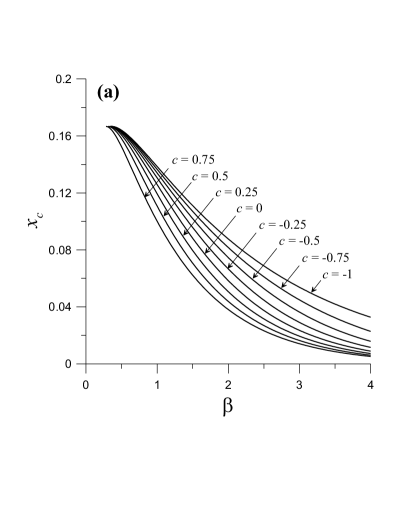
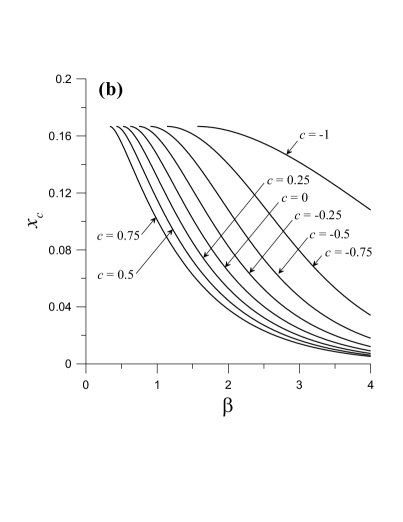
Fig. 2 shows the results of the numerical solution of Eq. (22) as a function of the inverse temperature $\beta$ at $f_{A}=0.5$ for various values of $c$ in the SN and SR cases. One can see that blockier RCs with higher values of $c$ have lower $x_{c}$ (hence, a lower free energy $\beta F/N=\log x_{c}$). At small values of $\beta$ (at high temperatures), all the curves terminate in the adsorption-desorption transition point where $x_{c}=x_{V}$ (recall that $x_{V}$ is the smallest singularity of $\Gamma_{V}(x)$ – the GF for the bulk chain, Eq. (23); for a simple cubic lattice one has $x_{V}=1/6$). The transition point, the critical value $\beta_{tr}$ of $\beta$, is therefore found from the equation

$$\det\left[\mathbf{E}-\mathbf{\Gamma}_{L}(x_{V})\mathbf{\Gamma}_{S}(x_{V})\right]=0.$$ (45)

The resulting value of $\beta_{tr}$ as a function of $f_{A}$, the relative weight of $A$-monomers in the sequence, is shown in Fig. 3. For $c<0$ the allowed range of $f_{A}$ narrows according to Eq. (8). In the case $c=-1$ it degenerates to a single point $f_{A}=0.5$. It can be seen that the aggregation of monomers into clusters shifts the transition points and the $x_{c}(\beta)$ curve towards lower values of $\beta$ (i.e., it favors adsorption) and this shift is more pronounced in the SR case.

Figure 3: Inverse adsorption transition temperature in the annealed approximation as function of A-monomer probability for $\varepsilon_{A}=-1$, $\varepsilon_{B}=0$ (a) $1$ (b) and different values of cluster parameters $c=-0.75$, $-0.5$, $-0.25$, $0$, $0.25$, $0.5$, $0.75$. The transition point for $f_{A}=0.5$ and $c=-1$ is shown by symbol $\oplus$.

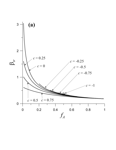
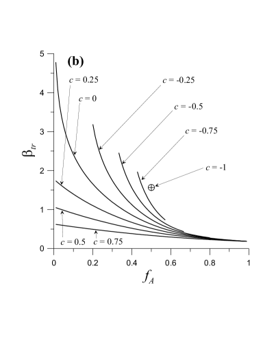
The equation for the transition point (45) has some similarity with the result obtained by Brun Brun:1999 . However, the latter contains only the largest eigenvalues, $\nu_{max}$, $\mu_{max}$, of the matrices $\mathbf{P}$ and $\mathbf{R}$, respectively. In our notation the equation of Brun has the form: $1-\Gamma_{L}(\nu_{max}x_{V})\Gamma_{S}(\mu_{max}x_{V})=0$. It gives the same result as Eq. (45) in the Bernoullian case ($c=0$), but overestimates $\beta_{tr}$ at $c<0$ and underestimates it at $c>0$, compared to our result.

Figs 4 and 5 show examples of the temperature dependence of the fraction of A- and B-contacts for the two cases SN and SR.

Figure 4: Fraction of A and B contacts in the annealed approximation for $f_{A}=0.5$, $\varepsilon_{A}=-1$, $\varepsilon_{B}=0$ and different values of cluster parameters $c=-1$, $-0.75$, $-0.5$, $-0.25$, $0$, $0.25$, $0.5$, $0.75$ as indicated (lines). Also shown are numerical results for $c=-1$ (crosses).

Figure 5: Fraction of A and B contacts in the annealed approximation for $f_{A}=0.5$, $\varepsilon_{A}=-1$, $\varepsilon_{B}=1$ and different values of cluster parameters $c=-1$, $-0.75$, $-0.5$, $-0.25$, $0$, $0.25$, $0.5$, $0.75$ as indicated (lines). Also shown are numerical results for $c=-1$ (crosses).

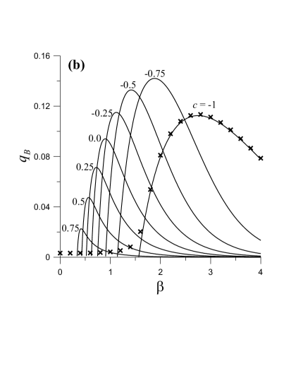
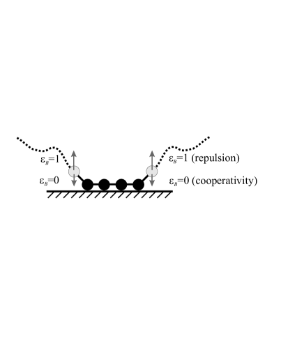
At $c=-1$, where the chain is a regular alternating copolymer, the ”annealed approximation” of course becomes exact and the results are in excellent agreement with the corresponding numerical results, which are also shown for comparison. The remaining difference is due to the finite chain length in the numerical calculations. This situation can be used to illustrate the main qualitative difference between the two cases SN and SR: The fraction of B-contacts (Figs. 4 b and 5 b) behaves differently depending on whether B-monomers are neutral or repelling. In the former case $q_{B}$ grows with $\beta$ whereas in the latter case it behaves nonmonotonically. The initial growth is caused by a cooperativity effect: B-monomers linked to adsorbed A-monomers have a higher probability to come into contact with the surface (see Fig. 6). In the SN case, such contacts are not penalized, hence the B-monomers are effectively attracted by the surface and $q_{B}$ continues to grow for all $\beta$. In the SR case, the cooperativity effect is counterbalanced by the increasing effect of the energy penalty on B-contacts, hence $q_{B}$ decreases again at high $\beta$.

Next we consider the curves corresponding to truly disordered chains with $c>-1$. Both in the SN and SR cases the fraction of A-contacts grows with increasing $\beta$ up to $q_{A}=1$, which is much higher than the expected fraction $f_{A}$ of A-stickers in the sequence (not necessarily adsorbed) for quenched disorder ($q_{A}(\beta\gg 1)\leq f_{A}$=0.5). At the same time, the fraction of B-contacts exhibits a nonmonotonic behaviour both in the SN and the SR case: Close to the transition point it grows, and then, after passing through a maximum, it decreases and virtually vanishes. This reflects the physical nature of the annealed approximation mentioned above: Any monomer can change its affinity to the surface (from negative to positive), if it is thermodynamically preferable for the system, and this is exactly the case at high $\beta$. Close to the transition point, the degree of A$\to$B conversion is small and neutral or repelling B-monomers come into contact with the surface due to the cooperativity effect described above; of course, for given chain statistic (given $f_{A}$ and $c$) and given inverse temperature $\beta$, $q_{B}$ is smaller in the SR case than in the SN case due to the additional penalty on B-contacts.

Figure 6: Illustration of cooperativity effect: Adsorbed train and its adjacent monomers.

This example demonstrates that the annealed approximation gives us essentially incorrect result regarding one of the most important conformational characteristics of adsorbed heteropolymer chains. Therefore it is necessary to improve on this approach. The Morita approximation (Sec. II.2) provides us with such a possibility.

III.2 ’Morita chains’ and Quenched chains

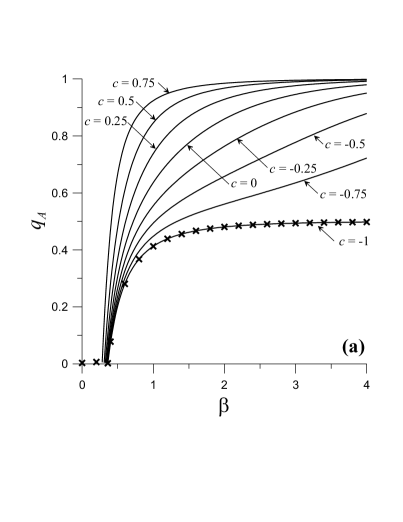
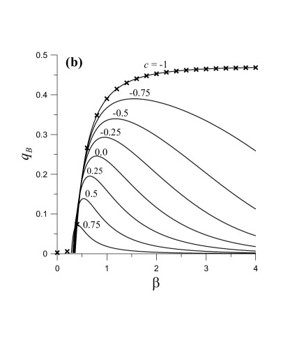
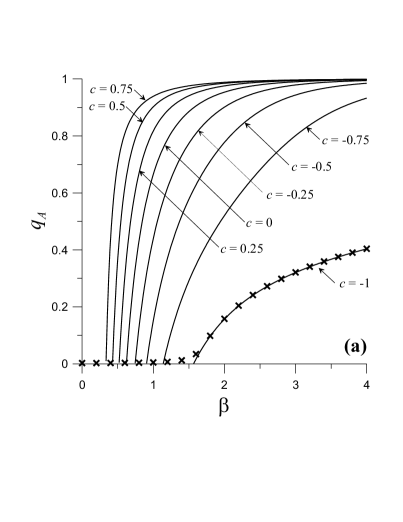
The objectives of the present work are not only to apply the Morita approximation for the problem of adsorption of correlated RCs, but also to estimate how good it can approximate the quenched (i.e. the real) system. The results obtained using the Morita approximation and the numerical approach (Sec. II.4) are thus presented together. We will use the following convention: The results obtained with the Morita approximation are shown as solid lines, whereas the data for the corresponding quenched systems are represented by symbols. Since our primary interest is to study the influence of correlations and the nature of the non-adsorbing monomer B on the RC adsorption properties, we set $f_{A}=0.5$ in this section. The results for $c=-1$ are not shown because they coincide with those obtained using the annealed approximation and have already been presented in Figs 4 and 5.

III.3 SN case

We consider first the SN case. Fig. 7 shows the temperature dependence of the fraction of A and B contacts for different values of the cluster parameter $c$. Both $q_{A}$ and $q_{B}$ grow with increasing $\beta$. The results for $q_{B}$ differ qualitatively from those obtained for all random copolymers ($c<-1$) in the annealed approximation, but they resemble those obtained for alternating copolymers ($c=-1$) in Fig. 4. The reason for the monotonic growth of $q_{B}$ is the absence of an energetic penalty on a B contact, combined with the cooperativity effect discussed earlier (Fig. 6). This effect explains the larger amount of B-contacts for RCs with lower $c$ at intermediate and strong adsorption (far from the transition point). Contrary to the annealed case (Fig. 4 a), the value of $q_{A}$ does not exceed $f_{A}$.

Figure 7: Fraction of A and B contacts calculated in the Morita approximation (lines) and using the transfer matrix approach (symbols) for $f_{A}=0.5$, $\varepsilon_{A}=-1$, $\varepsilon_{B}=0$ and different values of cluster parameters $c=-0.75$ ($\Box$), $-0.5$ ($\bigcirc$), $-0.25$ ($\Diamond$), $0$ ($\bigtriangleup$), $0.25$ ($\bigtriangledown$), $0.5$ ($+$), $0.75$ ($\star$).

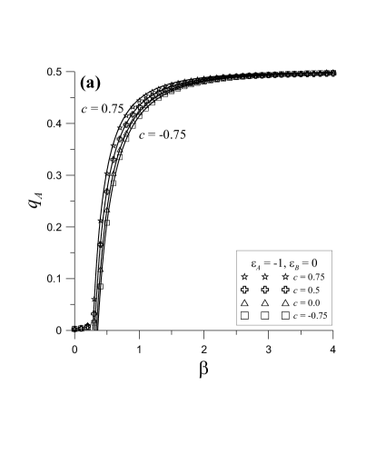
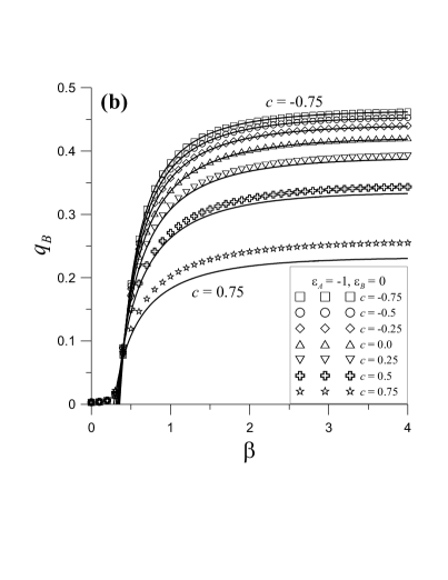
Comparing the results obtained using the Morita approximation and the numerical procedure, we have not only qualitative, but also a quantitative agreement. The curves for $q_{A}$ are predicted almost perfectly by the Morita approximation, the results are only very slightly overestimated. The $q_{B}$ curves are in reasonable agreement for $c\leq 0$, whereas for $c>0$, the Morita approximation underestimates $q_{B}$. This can be explained by the fact that the Morita copolymer has the possibility to adjust itself to the surface – A and B monomers can be redistributed between trains and loops.

III.4 SR case

Let us turn to the SR case. The results for the monomer-surface contacts $q_{A}$ and $q_{B}$ are presented in Fig. 8. As in the SN case, the fraction of A contacts grows with increasing $\beta$. Furthermore, $q_{A}$ decreases with decreasing cluster parameter $c$, in a much more pronounced fashion than for the SN case. In addition, the growth of $q_{A}$ with $\beta$ becomes slower with decreasing $c$.

Figure 8: Fraction of A and B contacts calculated in the Morita approximation (lines) and using the transfer matrix approach (symbols) for $f_{A}=0.5$, $\varepsilon_{A}=-1$, $\varepsilon_{B}=1$ and different values of cluster parameters $c=-0.75$ ($\Box$), $-0.5$ ($\bigcirc$), $-0.25$ ($\Diamond$), $0$ ($\bigtriangleup$), $0.25$ ($\bigtriangledown$), $0.5$ ($+$), $0.75$ ($\star$).

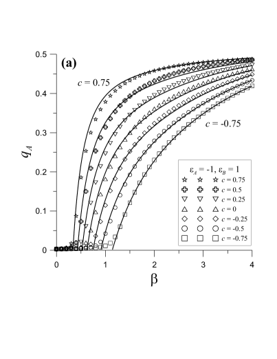
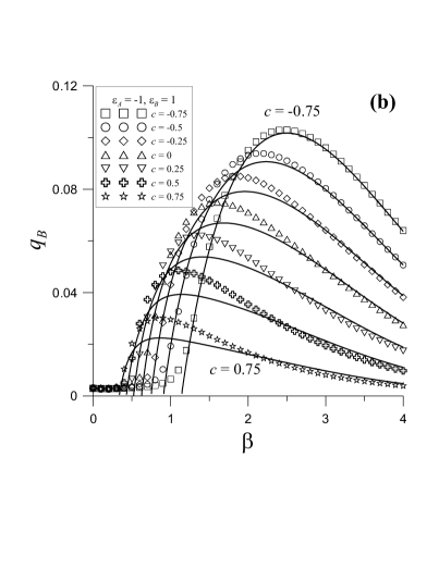
Unlike $q_{A}$, the fraction of (unfavourable) B contacts $q_{B}$ depends non-monotonically on the inverse temperature, Fig. 8 b. It increases just after the transition point, passes through a maximum and then decays. This behavior looks similar to that observed in the annealed approximation (both for the SN and SR cases, Figs. 4 b and 5 b), but its nature is very different: In the annealed case, B-monomers can convert to A ones, whereas both in the quenched case and in the Morita approximation a B$\to$A conversion is not possible. The initial growth of $q_{B}$ is due to the cooperative effect, Fig. 6, whereas the subsequent decay is caused by the increasing influence of the energy penalty on B-contacts. (Indeed, one can easily imagine the most probable (ground state) conformation in the $\beta\to\infty$ limit: All A-monomers are on the surface, all B-monomers are desorbed in loops.) It is worth noting that the Morita approximation seems to underestimate $q_{A}$ and overestimate $q_{B}$ at large $\beta$, i.e., small temperatures. This is counterintuitive, given that the Morita copolymer can adjust the A-B distribution on the sequence to the conformation to some extent. In fact, the discrepancy is simply an effect of the finite chain length in the numerical simulations. On the one hand, the cooperativity effect is reduced in the free tail, which reduces the number of B-contacts. On the other hand, A-monomers close to the tethered end can make contact with the surface more easily than A-monomers in the middle of the chain, which enhances the number of A-contacts.

The results presented in Fig. 8 lead us to the conclusion that the Morita approximation reproduces the fractions of A and B contacts in the quenched system reasonably well. The quantitative agreement is best for quasi-alternating RCs ($c=-0.5$ and $-0.75$). We suggest the following explanation of this effect: The Morita approximation reduces the initial heteropolymer problem to a homopolymer problem, thus “smoothing out” the monomer sequence of the RC. Obviously, a quasi-alternating RC can easily (and more realistically) be represented as a homopolymer with a monomer unit replaced by an effective one than a RC with $c>0$ where the blocky structure is essential (it could be better represented by a multiblock copolymer).

III.5 Adsorption transition point in the Morita approximation

Solving the problem of RC adsorption in the Morita approximation amounts to finding the solution of a system of three equations, Eqs. (32) and (33), with three unknowns: $y_{c}$, $\lambda$, and $\kappa$ (the partition function/the smallest singularity of $\Gamma(x)$ is then given by $x_{c}=y_{c}e^{\lambda f_{A}+\kappa f_{AA}}$).

We obtained that the Lagrange multipliers $\lambda$ abd $\kappa$ vanish in the the adsorption transition point: $\lambda(\beta_{tr})=\kappa(\beta_{tr})=0$. This implies that at the transition point, the Morita and the annealed approximation are equivalent. Hence, the transition point is the same for the Morita copolymer than for the annealed copolymer and is determined by Eq. (45), consistent with the conclusion of Caravenna and Giacomin Caravenna:2005 .

IV Summary and outlook

In the present work, the adsorption of a single two-letter RC chain with correlations in its monomer sequence onto a planar homogeneous surface was studied. One of the monomers (A) was always taken to be attracted to the surface whereas the other (B) – was neutral or repulsive (SN: sticky – neutral or SR: sticky – repulsive cases, respectively). The monomer sequence of the RC was modeled as a first order Markov chain, which is completely determined by two independent parameters. For the sake of convenience, we used as these parameters the probability for A monomers in the sequence, $f_{A}$, and the cluster parameter $c$ ($c=0$ - uncorrelated (Bernoullian), $c>0$ - quasi-blocky, and $c<0$ - quasi-alternating copolymer). To average the free energy over the sequence disorder , i.e., over the whole ensemble of monomer sequences, two approximations were employed: The annealed approximation and the Morita approximation. The partition function was calculated in the grand canonical ensemble using the GF approach which is based on the representation of an instantaneous conformation of the adsorbed chain as a sequence of independent non-interacting trains (adsorbed sequences) and loops flanked by tails.

In the framework of the annealed approximation, where the partition function, instead of its logarithm, is averaged over sequence disorder, a general approach for the calculation of the averaged partition function of the RC chain (in the form of the smallest singularity of the GF), the fraction of adsorbed monomers, and the transition point was developed. It was found that the annealed approximation cannot describe the quenched system correctly in the intermediate and strong adsorption regimes: For example, it strongly overestimates the fraction of contacts of adsorbing monomers, because of the possibility of A$\to$B monomer conversion. Nevertheless, the results for annealed chains are interesting in their own right since they describe the adsorption behavior of so-called two-state polymers (annealed copolymers).

The theory developed for the annealed approximation was then extended and combined with the Morita approximation. The latter approach is based on a constrained annealing procedure, where the quenched average is replaced by an annealed average subject to constraint on the moments of the monomer distribution. In our case, constraints on the first and the second moments were imposed.

To estimate the accuracy and validity of the Morita approximation, numerical calculations using a transfer matrix approach were carried out for the quenched system: Polymer chains of length $N=1000$ monomers were considered, for the given monomer statistics 100 realizations of random sequence were generated, for each realization the free energy and other observables were calculated and then averaged over the different realizations. The comparison of the results obtained using the Morita approximation and those for quenched system showed not only a qualitative but also a good quantitative correspondence, especially for quasi-alternating RCs (i.e., RCs with $c<0$).

It was shown that the fraction of adsorbed A-monomers grows monotonically as the inverse temperature $\beta$ increases, independently of the character of the interaction between the nonadsorbing B-monomer and the surface. In contrast, the fraction of adsorbed B-monomer behaves differently in SN and SR situations: In the former case, it increases with $\beta$, whereas in the latter case, it behaves nonmonotonically, exhibiting first a relatively rapid growth just above the adsorption transition point which is followed by decay at higher values of $\beta$.

The results of our calculations also indicate that both the annealed and the Morita approximations give the same adsorption transition point.

The special case $f_{A}=0.5$, $c=-1$ corresponds to the limiting situation of a quenched regular alternating AB-copolymer which can be solved exactly using the formal framework of the annealed approximation.

We remark that the approach developed in the present work can be applied in a straightforward way to other types of lattice models of polymers or to other geometries of adsorbing substrates. The key difference will be the calculation of GFs for adsorbed sequences (which is usually quite easy) and loops (which is a more sophisticated task). In the framework of the GF approach other interesting observables can be calculated as well, for example, the statistics of trains and loops. This will be the subject of future work.

Acknowlegdement

The financial support of the Deutsche Forschungsgemeinschaft (SFB 613) is gratefully acknowledged. A.P. thanks Russian Foundation for Basic Research (grant 08-03-00336-a).

Appendix A Calculation of $\Gamma(x)$ in the annealed approximation

Let us tranform the partition function (19) by exchanging the order of summation over conformations ($\omega$) and disorder ($\chi$) and taking the explicit form of the sequence probability $P(\chi)$, Eq (4) and later noting that the inner sum over all realisations of $\chi$ can be written in the matrix form:

$$\begin{split}\left\langle Z_{N}(\beta|\chi)\right\rangle&=\sum_{\chi}P(\chi)\sum_{\omega}\exp\left\{-\beta\sum_{i=1}^{N}\Delta_{i}\cdot\left[\chi_{i}\varepsilon_{A}+(1-\chi_{i})\varepsilon_{B}\right]\right\}\\ &=\sum_{\omega}\sum_{\chi}f_{\chi_{1}}\,e^{-\beta\Delta_{1}\cdot\left[\chi_{1}\varepsilon_{A}+(1-\chi_{1})\varepsilon_{B}\right]}\prod_{i=2}^{N}p_{\chi_{i-1},\,\chi_{i}}\,e^{-\beta\Delta_{i}\cdot\left[\chi_{i}\varepsilon_{A}+(1-\chi_{i})\varepsilon_{B}\right]}\\ &=\sum_{\omega}(f_{A}w_{A}^{\Delta_{1}},\,f_{B}w_{B}^{\Delta_{1}})\prod_{i=2}^{N}\left(\begin{array}[]{cc}p_{AA}w_{A}^{\Delta_{i}}&p_{AB}w_{B}^{\Delta_{i}}\\ p_{BA}w_{A}^{\Delta_{i}}&p_{BB}w_{B}^{\Delta_{i}}\end{array}\right)\cdot\left(\begin{array}[]{c}1\\ 1\end{array}\right)\\ &=\sum_{\omega}(\mathbf{W}^{\Delta_{1}}\mathbf{f})^{\mathrm{T}}\prod_{i=2}^{N}(\mathbf{PW}^{\Delta_{i}})\cdot\mathbf{e},\end{split}$$ (46)

where we have defined $w_{A}\equiv e^{-\beta\varepsilon_{A}}$, $w_{B}\equiv e^{-\beta\varepsilon_{B}}$, and

$$\mathbf{f}=\left(\begin{array}[]{c}f_{A}\\ f_{B}\end{array}\right),\quad\mathbf{W}=\left(\begin{array}[]{cc}w_{A}&0\\ 0&w_{B}\end{array}\right),\quad\mathbf{e}=\left(\begin{array}[]{c}1\\ 1\end{array}\right).$$ (47)

The final result in Eq. (46) does not depend on the sequence, i.e., we have effectively a homopolymer partition function (but of a somewhat complicated form). Since $\Delta_{i}$ can be either 0 or 1, each conformation will give us a product with the factors $\mathbf{f}^{\mathrm{T}}$ or $\mathbf{Wf}^{\mathrm{T}}_{1}$ (from the first monomer) and $\mathbf{P}$ and $\mathbf{R}\equiv\mathbf{PW}$ (from the monomers with $i=2,3\ldots N$ ) in a certain order corresponding to this conformation. Unfortunately, the matrices $\mathbf{P}$ and $\mathbf{R}$ do not commute and we are not able to simplify this expression by, for example, rewriting the sum over $\omega$ as a sum over the number of polymer contacts with the surface Soteros:2004 .

On the other hand, each adsorbed sequence (train), loop, or tail with the length $n$ contributes the factor $\mathbf{R}^{n}$, $\mathbf{P}^{n}$, or $\mathbf{P}^{n}$, respectively, in the partition function (46) (if we do not consider the first monomer) and we can use the sequence GF method (or the grand canonical ensemble technique) suggested by Lifson Lifson:1964 Introducing the GF of $\left\langle Z_{n}(\beta|\chi)\right\rangle$ (or grand canonical p.f.) $\Gamma(x)=\sum_{n=1}^{\infty}\left\langle Z_{n}(\beta|\chi)\right\rangle x^{n}$ and applying Lifson’s arguments Lifson:1964 we obtain the result (19) for $\Gamma(x)$.

Appendix B Calculation of loop generating function

In this Appendix, we briefly describe the calculation of the loop GF for the simple (6-choice) cubic lattice. First let us recall the ”definition” of the loop. A loop of length $n$

• starts and ends in the closest to the substrate lattice layer (site),

• contains NO monomers in the surface layer,

• the last, $n$th, monomer is followed by the step in the surface layer,

• all the effects (statistical weights) at the beginning of a loop may be attributed to the preceding adsorbed segment.

Figure 9: Decomposition of a loop on 6-choice simple cubic lattice.

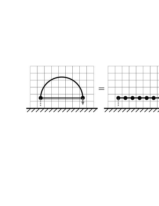
First, let us notice that the minimum loop length for the given model is equal to 1. To calculate the GF of a loop

$$\Gamma_{L}(x)=\sum_{n=1}^{\infty}\Omega_{L}(n)x^{n}$$ (48)

in the 6-choice simple cubic lattice, we have to take into account two possibilities (Fig. 9):

1. All the monomers of the loop are in the second layer (First ”term” in the rhs of Figure 9). The corresponding number of conformations is

   $$(z-2)^{n-1}$$

2. The first $k$ monomers are in the second layer, then a step into the third layer follows. We decompose this contribution in three terms: The first $k$ monomers, then loop starting from the second layer, which ends as soon as the first monomer reenters the second layer, and the rest. (Second ”term” in the rhs of Figure 9). The number of conformations is given by

   $$\sum_{k=1}^{n-2}\sum^{l=1}_{n-k-1}(z-2)^{k-1}\,\Omega_{L}(l)\,\Omega_{L}(n-k-l)\,,\quad n\geq 3$$

This gives us a recursion relation for $\Omega_{L}(n)$:

$$\Omega_{L}(n)=(z-2)^{n-1}+\sum_{k=1}^{n-2}\sum^{l=1}_{n-k-1}(z-2)^{k-1}\,\Omega_{L}(l)\,\Omega_{L}(n-k-l)\,,\quad n\geq 3\,.$$ (49)

By multiplying this equation by $x^{n}$ and summing from $n=3$ to infinity, we obtain the following recursion relation for the GF $\Gamma_{L}(x)$ (48)

$$\Gamma_{L}(x)-x-(z-2)x^{2}=\frac{x^{3}(z-2)^{2}}{1-(z-2)x}+\frac{x}{1-(z-2)x}\Gamma_{L}^{2}(x)\,.$$ (50)

Its solution is

$$\Gamma_{L}(x)=\frac{1}{2x}\left\{1-(z-2)x-\sqrt{(1-zx)[1-(z-4)x]}\right\}\,.$$ (51)

References

- (1) V Pande, A Yu Grosberg, and T Tanaka. Heteropolymer freezing and design: Towards physical models of protein folding. Rev. Mod. Phys., 72:259– 314, 2000.
- (2) R Bundschuh and T Hwa. Statistical Mechanics of secondary structures formed by random RNA sequences. Phys. Rev. E, 65:031903, 2002.
- (3) T Garel and C Monthus. Numerical study of the disordered Poland-Scheraga model of DNA denaturation. J. Stat. Mech.: Theor. Exp., page P06004, 2005.
- (4) A Chakraborty. Disordered heteropolymers: models for biomimetic polymers and polymers with frustrating quenched disorder. Phys. Rep., 342:1–61, 2001.
- (5) J U Sommer and M Daoud. Copolymers at selective interfaces. Europhysics Letters, 32:407–412, 1995.
- (6) A Trovato and A Maritan. A variational approach to the localization transition of heteropolymer at interfaces. Europhys. Lett., 46(3):301–306, 1999.
- (7) Z Y Chen. Localization of random copolymer at an interface. J. Chem. Phys., 112(19):8865–8671, 2000.
- (8) N A Denesyuk and I Ya Erukhimovich. Adsorption of a correlated random copolymer chain at a liquid-liquid interface. J. Chem. Phys., 113(9):3894–3900, 2000.
- (9) A Polotsky, F Schmid, and A Degenhard. Influence of sequence correlations on the adsortion of random copolymer onto homogeneous planar surface. J. Chem. Phys., 120(13):6246–6256, 2004.
- (10) A Polotsky, A Degenhard, and F Schmid. Polymer adsorption onto random planar surfaces: interplay of polymer and surface correlations. J. Chem. Phys., 121(10):4853–4864, 2004.
- (11) E Orlandini, A Rechnitzer, and S G Whittington. Random copolymers and the Morita approximation: polymer adsorption and polymer localization. J. Phys. A: Math. Gen., 35:7729–7751, 2002.
- (12) G Iliev, E Orlandini, and S G Whittington. Adsorption and localization of random copolymers subject to a force: The Morita approximation. Eur. Phys. J. B, 40:63–71, 2004.
- (13) J Alvarez, E Orlandini, C E Soteros, and S G Whittington. Higher order Morita approximations for random copolymer adsorption. J. Phys. A: Math. Theor., 40:F289–F298, 2007.
- (14) T Morita. Statistical Mechanics of Quenched Solid Solutions with Application to Magnetically Dilute Alloys. J. Math. Phys., 5(10):1401–1405, 1964.
- (15) R Kühn. Equilibrium ensemble approach to disordered systems I: general theory, exact results. Z. Phys. B, 100:231–242, 1996.
- (16) C E Soteros and S G Whittington. The statistical mechanics of random copolymers. J. Phys. A: Math. Gen., 37:R279–R325, 2004.
- (17) F Caravenna and G Giacomin. On Constrained Annealed Bounds for Pinning and Wetting Models. Elect. Comm. in Probab., 10:179 –189, 2005.
- (18) S Lifson. Partition Function of Linear Chain Molecules. J. Chem. Phys., 40(12):3705–3710, 1964.
- (19) D C Poland and H A Scheraga. Comparison of Theories of the Helix-Coil Transition in Polypeptides. J. Chem. Phys., 43(6):2071–2074, 1965.
- (20) T M Birshtein, A M Elyashevitch, and A M Skvortsov. The theory of intramolecular cross -coil transition. Mol. Biol. USSR, 5(1):78–90, 1971.
- (21) A Litan and S Lifson. Statistical-Mechanical Treatment of Multistranded Nucleotide Molecules. J. Chem. Phys., 42(7):2528–2532, 1965.
- (22) D C Poland and H A Scheraga. Phase Transitions in One Dimension and the Helix-Coil Transition in Polyamino Acids. J. Chem. Phys., 45(5):1456–1463, 1966.
- (23) T M Birshtein. Theory of Adsorption of Macromolecules: 1. The Desorption-Adsorption Transition Point. Macromolecules, 12(4):715–721, 1979.
- (24) T M Birshtein. Theory of Adsorption of Macromolecules: 2. Phase Transition in Adsorption: General Approach. Macromolecules, 16(1):45–50, 1983.
- (25) Ye B Zhulina, A M Skvortsov, and T M Birshtein. The theory of adsorption of regular block copolymers on the interphase. Vysokomol: Soedin. (USSR), 23(2):304–312, 1981.
- (26) Y Brun. The mechanism of copolymer retention in interactive polymer chromatography. I. Critical point of adsorption for statistical copolymers. J. Liq. Chrom. and Rel. Tech., 22(20):3027–3065, 1999.
- (27) Y Kafri, D Mukamel, and L Peliti. Why is the DNA Denaturation Transition First Order? Phys. Rev. Lett., 85(23):4988 –4991, 2000.
- (28) Y Kafri, D Mukamel, and L Peliti. Melting and unzipping of DNA. Eur. Phys. J. B, 27:135 –146, 2002.
- (29) T Garel, C Monthus, and H Orland. A simple model for DNA denaturation. Europhys. Lett., 55(1):132–138, 2001.
- (30) C Richard and A Guttmann. Poland-Scheraga Models and the DNA Denaturation Transition. J. Stat. Phys., 115(3/4):925–947, 2004.
- (31) M Muthukumar. Localized structures of polymers with long-range interactions. J. Chem. Phys., 104(2):691–700, 1996.
- (32) G Carri and M Muthukumar. Coupling Between Adsorption and the Helix-Coil Transition. Phys. Rev. Lett., 82(26):5405 –5408, 1999.
- (33) N Yoshinaga, E Kats, and A Halperin. On the Adsorption of Two-State Polymers. Macromolecules, 41(20):7744– 7751, 2008.
- (34) S Stepanow and A L Chudnowsky. The Green s function approach to adsorption of a random heteropolymer onto surfaces. J. Phys. A: Math. Gen., 35:4229–4238, 2002.
- (35) F R Gantmacher. The theory of matrices, vol. I. Chelsea, New York, 1959.
- (36) R J Rubin. J. Res. Natl. Bur. Stand. Sec. B, 69:301, 1965.
- (37) R J Rubin. J. Res. Natl. Bur. Stand. Sec. B, 70:237, 1966.
- (38) R J Rubin. Random-Walk Model of Chain-Polymer Adsorption at a Surface. J. Chem. Phys., 43(7):2392–2407, 1965.
- (39) G J Fleer, M A Cohen-Stuart, J M H M Scheutjens, T Cosgrove, and B Vincent. Polymers at Interfaces. Chapman and Hall, London, 1993.