A Spectral Analysis of the Sequence of Firing Phases in Stochastic Integrate-and-Fire Oscillators

Abstract

Integrate and fire oscillators are widely used to model the generation of action potentials in neurons. In this paper, we discuss small noise asymptotic results for a class of stochastic integrate and fire oscillators (SIFs) in which the buildup of membrane potential in the neuron is governed by a Gaussian diffusion process. To analyze this model, we study the asymptotic behavior of the spectrum of the firing phase transition operator. We begin by proving strong versions of a law of large numbers and central limit theorem for the first passage-time of the underlying diffusion process across a general time dependent boundary. Using these results, we obtain asymptotic approximations of the transition operator’s eigenvalues. We also discuss connections between our results and earlier numerical investigations of SIFs.

and

t1Supported in part by NSF grant DMS-05-04853. t2Supported in part by NSF RTG grant DMS-07-39164.

1 Introduction

The integrate and fire oscillator is widely used to model the behavior of the membrane potential in a neuron. Since its introduction by Lapicque [6] in 1907 it has been studied by many authors, see in particular Stein [13] and Knight [9]. The neurobiological derivation of the model is described in Tuckwell [18, 19] and a recent review of activity in the field appears in Burkitt [2, 3].

In this paper we use the following model for the stochastic integrate and fire oscillator (SIF). After starting at some time $t_{0}$ the membrane potential $X_{t}^{\varepsilon}$ evolves according to the stochastic differential equation

$$dX_{t}^{\varepsilon}=(-\gamma X_{t}^{\varepsilon}+I(t))dt+\varepsilon\,dW_{t}$$ (1)

until it reaches a (time-dependent) threshold level $g(t)$ at time

$$\tau_{1}^{\varepsilon}=\inf\{t\geq t_{0}:X_{t}^{\varepsilon}=g(t)\}.$$ (2)

At the hitting time $\tau_{1}^{\varepsilon}$ the membrane potential discharges, producing a voltage spike, and resets at a lower value

$$X_{(\tau_{1}^{\varepsilon})^{+}}^{\varepsilon}=h(t).$$ (3)

For $t\geq(\tau_{1}^{\varepsilon})^{+}$ the process $X_{t}^{\varepsilon}$ follows the SDE (1) until the second hitting time $\tau_{2}^{\varepsilon}=\inf\{t>\tau_{1}^{\varepsilon}:X_{t}^{\varepsilon}=g(t)\}$, and so on, yielding a sequence $\{\tau_{n}^{\varepsilon}:n\geq 1\}$ of hitting times.

Here $W_{t}$ is a standard one-dimensional Wiener process, and $\varepsilon\geq 0$ determines the intensity of the noise in the integrate and fire oscillator. The input function $I(t)$, the threshold function $g(t)$ and the reset function $h(t)$ are deterministic functions and will be regarded as given as part of the problem. The parameter $\gamma\geq 0$ gives the rate of leakage of current across the membrane. The terms “leaky” and “non-leaky” are sometimes used to describe the cases $\gamma>0$ and $\gamma=0$ respectively. The issue is to provide a concise description of the distribution of the random sequence $\{\tau_{n}^{\varepsilon}:n\geq 1\}$. It is of particular interest to describe how the distribution of the sequence $\{\tau_{n}^{\varepsilon}:n\geq 1\}$ responds to changes in one or more of the functions $I$, $g$ and $h$.

If all three functions are constant, then the inter-spike intervals $\tau_{n+1}^{\varepsilon}-\tau_{n}^{\varepsilon}$ form an independent, identically distributed sequence of random variables. A more interesting situation occurs when one of the functions undergoes a periodic modulation. In many applications the input function is taken to be of the form $I(t)=I_{0}+I_{1}\sin\omega t$. In other cases the threshold is taken to be of the form $g(t)=g_{0}+g_{1}\sin\omega t$. In this paper we will make the general assumption that the three functions $I$ and $g$ and $h$ all have the same period. Without loss of generality we will assume that the period is 1. Then the sequence of firing phases

$$\Theta_{n}^{\varepsilon}\equiv\tau_{n}^{\varepsilon}\quad\mbox{mod }1$$

determines a Markov chain $\{\Theta_{n}^{\varepsilon}:n\geq 1\}$ on the circle $\mathbb{S}=\mathbb{R}/\mathbb{Z}$.

When $\varepsilon=0$ the process $X_{t}^{0}$ is given by an ordinary differential equation. Therefore the hitting times are given by $\tau_{n+1}^{0}=f(\tau_{n}^{0})$ for some deterministic function $f$ satisfying $f(t+1)=f(t)+1$, and the firing phases are given by $\Theta_{n+1}^{0}=\tilde{f}(\Theta_{n}^{0})$ where $\tilde{f}(\theta)\equiv f(\theta)$ mod 1. In settings where either the input function $I(t)$ or the threshold function $g(t)$ is of the form $A+B\sin 2\pi t$ (and the other two functions are constant), the dynamical system on $\mathbb{S}$ generated by iterating $\tilde{f}$ has been studied by Rescigno, Stein, Purple and Poppele [11], Knight [9], Glass and Mackey [5] and Keener, Hoppensteadt and Rinzel [8]. Of particular interest are the regions in the $(A,B)$ parameter space giving rise to phase-locked behavior, and the bifurcation scenario as $A$ and $B$ are varied.

When $\varepsilon>0$ the deterministic hitting time function $f$ is replaced by the first passage-time density function

$$p^{\varepsilon}(t|t_{0}):=\frac{\partial}{\partial t}\mathbb{P}(\tau_{n}^{\varepsilon}\leq t|\tau_{n-1}^{\varepsilon}=t_{0})$$

and $\tilde{f}$ is replaced the projection $\tilde{p}(\theta|\theta_{0})$, say, of $p^{\varepsilon}(t|t_{0})$ onto the circle $\mathbb{S}$. The behavior of the Markov chain $\{\Theta_{n}^{\varepsilon}:n\geq 1\}$ may be studied via its transition operator $T^{\varepsilon}$ given by

$$T^{\varepsilon}\phi(\theta)=\mathbb{E}\left(\phi(\Theta_{1}^{\varepsilon})\big{|}\Theta_{0}^{\varepsilon}=\theta\right)=\int_{\mathbb{S}}\phi(\theta)\tilde{p}^{\varepsilon}(\theta|\theta_{0})d\theta=\sum_{m}\int_{\mathbb{S}}\phi(\theta)p^{\varepsilon}(\theta+m|\theta_{0})d\theta$$

for $\phi$ in the class $B(\mathbb{S})$ of bounded measurable functions on $\mathbb{S}$. For any $\varepsilon>0$ the transition densities $\tilde{p}^{\varepsilon}(\theta|\theta_{0})$ are bounded away from zero, so that the Markov chain $\{\Theta^{\varepsilon}_{n}:n\geq 1\}$ is uniformly ergodic and has a unique stationary probability distribution. The compact operator $T^{\varepsilon}$ captures the essential dynamics of $\Theta_{n}^{\varepsilon}$, and hence its spectrum is of primary interest in quantifying the transient and asymptotic behavior of the system.

In a sequence of papers Tateno [14, 15] and Tateno and Jimbo [16] consider the effect of small noise on the deterministic bifurcation scenarios considered earlier. The papers [14, 15, 16] contain numerical calculations of the leading eigenvalues of the transition operator $T^{\varepsilon}$. These calculations suggest a qualitative change in the small noise behavior of the leading eigenvalues near the location of the deterministic bifurcation. The calculations in [14, 15, 16] involve numerical approximations in two places. Firstly, since there no explicit formula for the first-passage density $p(t|t_{0})$ except in a few special cases, numerical techniques are used to solve an integral equation for $p(t|t_{0})$, following the method proposed by Buonocore, Nobile and Ricciardi [1]. Secondly, the circle $\mathbb{S}$ is replaced by a finite set of points. Thus the operator $T^{\varepsilon}$ acting on $B(\mathbb{S})$ is approximated by a finite-dimensional stochastic matrix.

In this paper we obtain rigorous results on the asymptotic behavior of the spectrum of the operator $T^{\varepsilon}$ as $\varepsilon\to 0$. The first main result gives a Gaussian approximation for the first-passage density $p^{\varepsilon}(t|t_{0})$ as $\varepsilon\to 0$. This result does not use the assumption of periodicity, and is valid for any $C^{2}$ functions $I(t)$ and $g(t)$ and starting position $X^{\varepsilon}(t_{0})=x_{0}<g(t_{0})$, under the condition that the deterministic hitting time is finite and that the deterministic trajectory crosses the threshold transversally. For details see Section 2 and especially Theorem 1. This result can be applied in the periodic setting to show that the Markov chain $\{\Theta^{\varepsilon}_{n}:n\geq 1\}$ can be well approximated by small Gaussian perturbations away from the deterministic mapping $\tilde{f}$. The estimate in Theorem 1 is sufficiently strong that the techniques in Mayberry [10], which deals with small Gaussian perturbations of circle maps, can be applied here also. In the simplest case where the deterministic mapping $\tilde{f}$ is continuous and has one stable fixed point $\theta_{s}$ attracting all orbits except the one started at one unstable fixed point $\theta_{u}$, the limiting eigenvalues of $T^{\varepsilon}$ can be calculated explicitly in terms of $\tilde{f}^{\prime}(\theta_{s})$ and $\tilde{f}^{\prime}(\theta_{u})$, see Theorem 2 in Section 3. This result can be extended to the case where $\tilde{f}$ is continuous and phase-locked, see Remark 3. In many examples of SIF the deterministic mapping $\tilde{f}$ has a finite set of discontinuities, and this case is treated in Section 4. The main result, Theorem 3, deals with the case where $\tilde{f}$ is phase-locked and where the discontinuities are well away from the phase locked orbit. (This rather vague assertion is made precise in condition (D3) of Theorem 3.)

Tateno and Jimbo [16] consider the leaky SIF with constant input $I$, periodically modulated threshold $g(t)=1+k\sin 2\pi$ and constant reset level $0$. Using a $100\times 100$ stochastic matrix in place of the operator $T^{\varepsilon}$, they produce plots of the leading eigenvalues for various small values of the noise intensity $\varepsilon$. In Section 5, we indicate how, in the phase-locked setting, our results may be applied to give a theoretical interpretation of the $\varepsilon\to 0$ behavior seen in some of the figures of [16].

Finally, Sections 6, 7 and 8 contains the proofs for the results in Sections 2, 3 and 4 respectively.

2 First passage times

The results in this section do not use periodicity, and are valid for general $C^{2}$ functions $I(t)$ and $g(t)$, and for all $\gamma\geq 0$.

Denote by $\mathbb{P}^{t_{0},x_{0}}$ the law of the diffusion process $\{X_{t}^{\varepsilon}:t\geq t_{0}\}$ satisfying

$$dX_{t}^{\varepsilon}=(-\gamma X_{t}^{\varepsilon}+I(t))dt+\varepsilon\,dW_{t}$$ (4)

with initial condition $X_{t_{0}}^{\varepsilon}=x_{0}$. For $x_{0}<g(t_{0})$ define the first passage time

$$\tau^{\varepsilon}=\inf\{t\geq t_{0}:X_{t}^{\varepsilon}=g(t)\}$$

of the process $X_{t}^{\varepsilon}$ across the threshold $g(t)$. In this section we will consider the behavior of the distribution of $\tau^{\varepsilon}$, and in particular its density function

$$p^{\varepsilon}(t|t_{0},x_{0})=\frac{\partial}{\partial t}\mathbb{P}^{t_{0},x_{0}}(\tau^{\varepsilon}\leq t),$$

as $\varepsilon\to 0$.

Let $\xi(t)=\xi(t|\,t_{0},x_{0})$ denote for $t\geq t_{0}$ the solution to the noise free ($\varepsilon=0$) equation (4) with initial condition $\xi(t_{0})=x_{0}<g(t_{0})$. Thus

$$\xi(t|t_{0},x_{0})=e^{-\gamma(t-t_{0})}x_{0}+\int_{t_{0}}^{t}e^{-\gamma(t-s)}I(s)\,ds.$$

For $x_{0}<g(t_{0})$ let

$$f(t_{0},x_{0})=\inf\{t\geq t_{0}:\xi(t|t_{0},x_{0})=g(t)\}$$

denote the deterministic hitting time. If $f(t_{0},x_{0})<\infty$, define

$$m(t_{0},x_{0})=-\gamma g(f(t_{0},x_{0}))+I(f(t_{0},x_{0}))-g^{\prime}(f(x_{0},t_{0})).$$

Thus $m(t_{0},x_{0})$ measures the difference in slopes when the deterministic solution $\xi(t|t_{0},x_{0})$ first meets the threshold $g(t)$. Since $x_{0}<g(t_{0})$, the deterministic solution hits from below and so $m(t_{0},x_{0})\geq 0$. The deterministic solution crosses the threshold transversally if and only if $m(t_{0},x_{0})>0$. Now define the set

$${\cal G}=\{(t_{0},x_{0}):x_{0}<g(t_{0})\mbox{ and }f(t_{0},x_{0})<\infty\mbox{ and }m(t_{0},x_{0})>0\}.$$

of initial conditions $(t_{0},x_{0})$ for which the deterministic trajectory crosses the threshold function transversally at the finite time $f(t_{0},x_{0})$.

Proposition 1.

${\cal G}$ is an open set and $f\in C^{2}({\cal G},\mathbb{R})$.

The proofs of the results in this section can be found in Section 6. Our next result gives a uniform bound on the deviation of $\tau^{\varepsilon}$ away from the deterministic crossing time $f(t_{0},x_{0})$.

Proposition 2.

Let $G$ be a compact subset of ${\cal G}$. Then for any $\delta>0$ there are constants $M_{\delta}$ and $K_{\delta}$ such that

$$\mathbb{P}^{t_{0},x_{0}}(|\tau^{\varepsilon}-f(t_{0},x_{0})|>\delta)\leq M_{\delta}\varepsilon\,e^{-K_{\delta}/\varepsilon^{2}}$$

for all $(t_{0},x_{0})\in G$.

For $(t_{0},x_{0})\in{\cal G}$ define

$$\sigma^{2}(t_{0},x_{0})=\left\{\begin{array}[]{cl}(1-e^{-2\gamma(f(t_{0},x_{0})-t_{0})})/2\gamma&\hskip 21.68121pt\mbox{ if }\gamma>0,\\[4.30554pt] f(t_{0},x_{0})-t_{0}&\hskip 21.68121pt\mbox{ if }\gamma=0.\end{array}\right.$$

Notice that $\varepsilon^{2}\sigma^{2}(t_{0},x_{0})$ is the variance of $X_{t}^{\varepsilon}$ at the moment $t=f(t_{0},x_{0})$ of noise-free intersection. Define

$$\sigma_{\tau}^{2}(t_{0},x_{0})=\frac{\sigma^{2}(t_{0},x_{0})}{m^{2}(t_{0},x_{0})}$$ (5)

and

$$p_{\tau}(t|t_{0},x_{0})=\frac{1}{\sqrt{2\pi\sigma^{2}_{\tau}(t_{0},x_{0})}}e^{-t^{2}/2\sigma^{2}_{\tau}(t_{0},x_{0})},$$

so that $p_{\tau}(t|t_{0},x_{0})$ is the density at $t$ of a $N(0,\sigma^{2}_{\tau}(t_{0},x_{0}))$ normal random variable. With this notation in hand, we can state the main result of this section.

Theorem 1.

Let $G$ be a compact subset of ${\cal G}$. Then there exist finite positive constants $\delta$, $\sigma_{1}$, $K$ and $\varepsilon_{0}$ (depending on $G$) so that

$$\sup_{(t_{0},x_{0})\in G}|\varepsilon p^{\varepsilon}(f(t_{0},x_{0})+u|t_{0},x_{0})-p_{\tau}(u/\varepsilon|t_{0},x_{0})|\leq K\varepsilon e^{-u^{2}/2\varepsilon^{2}\sigma_{1}^{2}}$$ (6)

for all $\varepsilon<\varepsilon_{0}$, $|u|\leq\delta$.

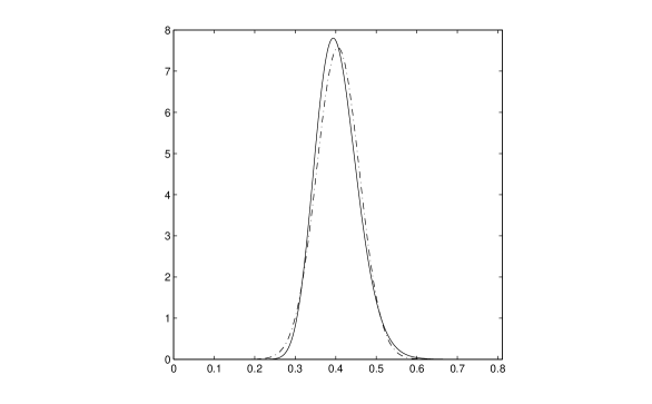
Figure 1: First passage-time pdf for $dX_{t}=(-X_{t}+2)dt+.1dW_{t}$, $X_{0}=.5$, across $g(t)=1$. Dashed line: Gaussian approximation of Theorem 1 with mean $\ln(1.5)\approx.4055$ and standard deviation $\sqrt{5/1800}\approx 0.0527$. Solid: Numerical approximation obtained by solving integral equation from [1]

Remark 1.

Under $\mathbb{P}^{t_{0},x_{0}}$ the centered and scaled hitting time $(\tau^{\varepsilon}-f(t_{0},x_{0}))/\varepsilon$ has density $\varepsilon p^{\varepsilon}(f(t_{0},x_{0})+\varepsilon t|t_{0},x_{0})$ at $t$. Putting $u=\varepsilon t$ in Theorem 1 gives the result that under $\mathbb{P}^{t_{0},x_{0}}$

$$\frac{\tau^{\varepsilon}-f(t_{0},x_{0})}{\varepsilon}\Rightarrow N(0,\sigma^{2}_{\tau}(t_{0},x_{0}))\quad\mbox{ as }\varepsilon\to 0,$$ (7)

or more informally

$$\tau^{\varepsilon}\approx N(f(t_{0},x_{0}),\varepsilon^{2}\sigma^{2}_{\tau}(t_{0},x_{0}))\quad\mbox{ as }\varepsilon\to 0.$$

Figure 1 shows the densities of $\tau^{\varepsilon}$ and $N(f(t_{0},x_{0}),\varepsilon^{2}\sigma_{\tau}(t_{0},x_{0}))$ for an example with $\varepsilon=0.1$. Of course the result in Theorem 1 is much stronger than (7) since it gives locally uniform convergence of densities, rather than just convergence in distribution. This extra strength will be important for the spectral analysis results in the next two sections.

Remark 2.

In equation (5) the difference in slopes $m(t_{0},x_{0})$ at the point of deterministic intersection is used to convert the variance $\sigma(t_{0},x_{0})$ in the spatial dimension into the variance $\sigma_{\tau}(t_{0},x_{0})$ in the temporal dimension. A heuristic observation of this conversion factor appears in Stein [13].

3 Transition Operator for the SIF

We now return to the setting of SIFs. The functions $I(t)$, $g(t)$ and $h(t)$ are assumed to be $C^{2}$ and periodic with period 1. Also $h(t)<g(t)$ for all $t$, and $\gamma\geq 0$. The deterministic solution is

$$\xi(t|t_{0},x_{0})=e^{-\gamma(t-t_{0})}x_{0}+\int_{t_{0}}^{t}e^{-\gamma(t-s)}I(s)\,ds.$$

If $\gamma=0$, then the assumption $\int_{0}^{1}I(s)\,ds>0$ implies that $\xi(t|t_{0},x_{0})\to\infty$ as $t\to\infty$ and so the deterministic hitting $f(t_{0},x_{0})$ is finite. If $\gamma>0$ then $\left|\xi(t|t_{0},x_{0})-\overline{\xi}(t)\right|\to 0$ as $t\to\infty$ where

$$\overline{\xi}(t)=\int_{-\infty}^{t}e^{-\gamma(t-s)}I(s)\,ds=\frac{1}{1-e^{-\gamma}}\int_{t-1}^{t}e^{-\gamma(t-s)}I(s)\,ds=\frac{1}{e^{\gamma}-1}\int_{0}^{1}e^{\gamma u}I(t+u)\,du.$$

In order to ensure that crossings for the noise free system occur in a nice enough fashion we impose the following conditions on the functions $I(t)$ and $g(t)$:

(A)

$\left\{\begin{array}[]{cl}\max\{\overline{\xi}(t)-g(t):0\leq t\leq 1\}>0&\mbox{ if }\gamma>0\\[4.30554pt] \displaystyle{\int_{0}^{1}I(s)ds>0}&\mbox{ if }\gamma=0\end{array}\right.$

(B)

$-\gamma g(t)+I(t)-g^{\prime}(t)>0$ for all $t$

Note that (A) implies that $f(t_{0},x_{0})<\infty$ whenever $x_{0}<g(t_{0})$, and then (B) implies that $m(t_{0},x_{0})>0$. Therefore ${\cal G}=\{(t_{0},x_{0}):x_{0}<g(t_{0})\}$, and we can apply our results on first passage densities from Section 2 using the compact set $G=\{(s,h(s)):0\leq s\leq 1\}$. We always take $x_{0}=h(t_{0})$, so we write $p^{\varepsilon}(t|t_{0})=p^{\varepsilon}(t|t_{0},h(t_{0}))$, $f(t_{0})=f(t_{0},h(t_{0}))$, $\sigma_{\tau}^{2}(t_{0})=\sigma^{2}_{\tau}(t_{0},h(t_{0}))$, etc. Proposition 1 implies that $f\in C^{2}(\mathbb{R})$, and clearly $f(t+1)=f(t)+1$ for all $t\in\mathbb{R}$. Theorem 1 implies that when $\varepsilon>0$ is small, we have the approximation

$$\tau_{n}^{\varepsilon}\approx f(\tau_{n-1}^{\varepsilon})+\varepsilon\sigma_{\tau}(\tau_{n-1}^{\varepsilon})\chi_{n}$$ (8)

where $\{\chi_{n}:n\geq 1\}$ is a sequence of independent $N(0,1)$ random variables.

The sequence of firing phases $\{\Theta_{n}^{\varepsilon}:n\geq 1\}$ is a Markov chain on the circle $\mathbb{S}=\mathbb{R}/\mathbb{Z}$ with transition density function

$$\tilde{p}^{\varepsilon}(\theta|\theta_{0})=\sum_{m\in\,\mathbb{Z}}p^{\varepsilon}(\theta+m|\theta_{0})$$ (9)

for all $\theta,\theta_{0}\in\mathbb{S}$. Looking at (8), we may expect that the study of $\{\Theta_{n}^{\varepsilon}:n\geq 1\}$ should be similar to the study of the chain

$$Y_{n}^{\varepsilon}=f(Y_{n-1}^{\varepsilon})+\varepsilon\sigma_{\tau}(Y_{n-1}^{\varepsilon})\chi_{n}\hskip 14.45377pt\mod 1.$$ (10)

Spectral properties of the transition operator for Markov chains of the form (10) were developed in Mayberry [10]. Here, we prove a similar result for the transition operator $T^{\varepsilon}$ of the chain $\{\Theta_{n}^{\varepsilon}:n\geq 1\}$.

Theorem 2.

Let $\{\Theta_{n}^{\varepsilon}:n\geq 1\}$ be the sequence of firing phases for a period 1 SIF with $C^{2}$ input, threshold and reset functions $I(t)$, $g(t)$ and $h(t)$. Assume the conditions (A) and (B). Suppose that the deterministic phase return map

$$\tilde{f}\equiv f\quad\mod\,1$$

has a stable fixed point $\theta_{s}$ and an unstable fixed point $\theta_{u}$, and that $\tilde{f}^{n}(\theta)\rightarrow\theta_{s}$ for all $\theta\in\mathbb{S}\setminus\{\theta_{u}\}$. Let $T^{\varepsilon}$ denote the transition operator for $\{\Theta_{n}^{\varepsilon}:n\geq 1\}$. Then for any $r>0$ and $\varepsilon$ sufficiently small, we can write $T^{\varepsilon}=T_{lp}^{\varepsilon}+T_{up}^{\varepsilon}$ where $\|T_{lp}^{\varepsilon}\|_{\infty}<r$ and any eigenvalue of $T_{up}^{\varepsilon}$ with modulus greater than $r$ is of one of the two forms $c_{s}^{n}+O(\varepsilon)$ or $|c_{u}|^{-1}c_{u}^{-n}+O(\varepsilon)$ for some $n\geq 0$, where $c_{s}=f^{\prime}(\theta_{s})$ and $c_{u}=f^{\prime}(\theta_{u})$.

The proof of this result can be found in Section 7. The result says that $c_{s}^{n}$ and $|c_{u}|^{-1}c_{u}^{-n}$ are the limiting eigenvalues of $T^{\varepsilon}$ in the sense that for any $r>0$, $T^{\varepsilon}$ has sequences of $r$-pseudoeigenvalues which converge to $c_{s}^{n}$ and $|c_{u}|^{-1}c_{u}^{-n}$ as $\varepsilon\to 0$ (see Trefethen and Embree [17] for definitions of pseudoeigenvalues).

Remark 3.

Theorem 2 can be extended to the case where $\tilde{f}$ has periodic orbits. Consider an orbit $\{\theta_{1},\theta_{2},\ldots,\theta_{\kappa}\}$ of period $\kappa\geq 1$ and let $c=f^{\prime}(\theta_{1})f^{\prime}(\theta_{2})\cdots f^{\prime}(\theta_{\kappa})$ denote the product of the derivatives of $f$ along the periodic orbit. If the orbit is stable, so that $|c|<1$, then it contributes limiting eigenvalues $(c^{n})^{1/\kappa}$ for $n\geq 0$. If the orbit is unstable, so that $|c|>1$, then it contributes limiting eigenvalues $(|c|^{-1}c^{-n})^{1/\kappa}$. Here all the $\kappa$th roots are included as limiting eigenvalues. The proof in this more general setting combines the method of proof of Theorem 2 with techniques used in the proof of [10, Theorem 1], and is left to the reader. Moreover, the methods used in [10, Theorem 2] can be applied here to give information about the associated eigenfunctions.

4 Discontinuous Case

Tateno and Jimbo [16] consider several cases of SIFs in which $f$ is well defined, but Assumption (B) fails and $f$ is discontinuous at some $\theta^{*}\in\mathbb{S}$. In this section, we will discuss extensions of Theorem 2 to this situation. As before, for $h(t_{0})<g(t_{0})$ we define $f(t_{0})=\inf\{t\geq t_{0}:\xi(t|t_{0})=g(t)\}<\infty$, but now we also define $f^{*}(t_{0})=\inf\{t>t_{0}:\xi(t|t_{0})>g(t)\}$. Thus $f(t_{0})$ is the time of first hitting of the threshold, and $f^{*}(t_{0})$ is the time of first crossing of the threshold. We keep (A) unchanged, but replace condition (B) with

(B’)

There is a finite set $D\subset[0,1)$ (possibly empty) such that $-\gamma g(f(t_{0}))+I(f(t_{0}))-g^{\prime}(f(t_{0}))>0$ for all $t_{0}\in[0,1)\setminus D$.

(C’)

For each $t_{0}\in D$ either

(i)

$f^{*}(t_{0})=f(t_{0})$; or else

(ii)

$f^{*}(t_{0})>f(t_{0})$ and $g(t)>\xi(t|t_{0})$ for $f(t_{0})<t<f^{*}(t_{0})$.

Figure 2: Examples of the behavior described in (C’). In both cases $\gamma=1$, $I(t)\equiv 1.4$, $g(t)=1+B\sin 2\pi t$ and $h(t)\equiv 0$. Case (i) on the left has $B=.0629,t_{0}=-.2527$ giving $f(t_{0})=f^{*}(t_{0})=1.0251$. Case (ii) on the right has $B=.3,t_{0}=.0863$ giving $f(t_{0})=.8087$, $f^{*}(t_{0})=1.473$.

Notice that (A) implies that $f(t_{0})\leq f^{*}(t_{0})<\infty$ for all $t_{0}$, and that (B’) implies that Proposition 2 can be applied to any compact subset of $[0,1]\setminus D$. In case (C’)(i) the deterministic trajectory $\xi(t|t_{0})$ crosses the threshold $g(t)$ at $t=f(t_{0})$, and $f$ is continuous (but not differentiable) at $t_{0}$; and in case (C’)(ii) $\xi(t|t_{0})$ touches $g(t)$ at $t=f(t_{0})$ and then does not intersect again until it crosses at time $t=f^{*}(t_{0})$, and $f$ is discontinuous at $t_{0}$. Examples of the behavior described in (C’) are given in Figure 2.

We begin with the following extension of Proposition 2. Proofs for the results in this section can be found in Section 8.

Proposition 3.

Suppose that $f$ satisfies (A), (B’) and (C’), and $D\neq\emptyset$. Then for all $\delta>0$ there exist $\tilde{\delta}>0$ and $K,M$ such that

$$\mathbb{P}^{t}(d(\tau^{\varepsilon},\{f(t_{0}),f^{*}(t_{0})\})>\delta)\leq\varepsilon Me^{-K/\varepsilon^{2}}$$

whenever $|t-t_{0}|<\tilde{\delta}$ for some $t_{0}\in D$.

The assumptions in our final theorem are not the most general ones possible, but the result is sufficient to treat the examples in the next section and to give the reader the indication of how Theorem 2 (see also Remark 3) can be extended to discontinuous settings. The conditions may seem awkward, but we will see in the next section that they are easy to verify numerically in examples of interest.

Theorem 3.

Suppose that (A), (B’), and (C’) are satisfied and in addition that $\tilde{f}=f$ mod 1 satisfies the conditions

(D1)

$\tilde{f}$ has a periodic orbit $P=\{\theta_{1},\ldots,\theta_{\kappa}\}$ in $\mathbb{S}\setminus D$ for some $\kappa\geq 1$ and

$$|\tilde{f}^{\prime}(\theta_{1})\tilde{f}^{\prime}(\theta_{2})\cdots\tilde{f}^{\prime}(\theta_{\kappa})|<1.$$

(D2)

$\tilde{f}^{n}(\theta)\to P$ as $n\to\infty$ for all $\theta\in\mathbb{S}$.

(D3)

$\tilde{f}^{-\ell}(D)=\emptyset$ for some $\ell\geq 1$ and $\tilde{f}^{i}(E)\cap D=\emptyset$ for $0\leq i\leq\ell-1$, where $E=\tilde{f}(D)\cup\tilde{f}^{*}(D)$.

Let $T^{\varepsilon}$ denote the transition operator for $\Theta_{n}^{\varepsilon}$. Then for any $r>0$ and $\varepsilon$ sufficiently small, we can write $T^{\varepsilon}=T_{lp}^{\varepsilon}+T_{up}^{\varepsilon}$ where $\|T_{lp}^{\varepsilon}\|_{\infty}<r$ and any eigenvalue of $T_{up}^{\varepsilon}$ with modulus greater than $r$ is of the form $(c^{n})^{1/\kappa}+O(\varepsilon)$ for $n\geq 0$, where $c=\tilde{f}^{\prime}(\theta_{1})\tilde{f}^{\prime}(\theta_{2})\cdots\tilde{f}^{\prime}(\theta_{\kappa})=(\tilde{f}^{\kappa})^{\prime}(\theta_{i})$ for any $i\in\{1,\ldots,\kappa\}$.

5 Examples from Tateno and Jimbo

We now apply our spectral results to the examples considered in [16]. There, the authors consider leaky SIFs with constant input $I(t)\equiv I$, threshold $g(t)=1+k\sin 2\pi t$, and reset $h(t)\equiv 0$. Since $\overline{\xi}(t)=I/\gamma$ the condition (A) becomes

$$I/\gamma>1-k.$$ (11)

The transversality condition (B) is now

$$-\gamma(1+k\sin 2\pi t)+I-2\pi k\cos 2\pi t>0\quad\quad\mbox{ for all }t$$

or equivalently

$$I/\gamma-1>k\sqrt{4\pi^{2}/\gamma^{2}+1}.$$ (12)

If condition (B) fails, then there is a point of tangency on the threshold curve which leads to a point with the property described in (C’)(i) or (C’)(ii). In any case, assuming (A) holds, we obtain $f(t_{0})=\inf\{t\geq t_{0}:h(t)=t_{0}\}$ where

$$h(t)=t+\frac{1}{\gamma}\log\left(1-\frac{\gamma}{I}(1+k\sin 2\pi t)\right).$$

If $h^{\prime}(t)>0$ for all $t$ then $f=h^{-1}$ is a smooth function. However, strict local maxima of $h$ give rise to discontinuities in $f$. Moreover periodic orbits of the induced mapping $\tilde{f}$ on $\mathbb{S}$ can be found using the facts that if $h^{\kappa}(t_{0})=t_{0}$ mod 1 then $f^{\kappa}(t_{0})=t_{0}$ mod 1 and $(f^{\kappa})^{\prime}(t_{0})=1/(h^{\kappa})^{\prime}(t_{0})$. The plots of $\tilde{f}$ and the numbers in the examples below are obtained using the explicit formula for $h$.

Tateno and Jimbo take $\gamma=1/12.8$ and various values of $I$ and $K$.

Figure 3: Plot of $\tilde{f}$ for $I=1,k=0.1,\gamma=1/12.8$

Example 1. Taking $I=1$ and $k=0.1$ gives the map $\tilde{f}$ in Figure 3, which satisfies the conditions of Theorem 2. There is a stable fixed point at $0.5622$ with $\tilde{f}^{\prime}(0.5622)=0.6142$ and an unstable fixed point at $0.9379$ with $\tilde{f}^{\prime}(0.9379)=2.6898$. All orbits starting at $\theta_{0}\neq 0.9379$ converge to $0.5622$ so by Theorem 2 the limiting eigenvalues are $\{0.6142^{n}:n\geq 0\}\cup\{2.6898^{-n-1}:n\geq 0\}=\{1,0.6142,0.3772,0.3718,0.2317,\ldots\}$

Figure 4: Plot of $\tilde{f}$ for $I=1,k=0.35,\gamma=1/12.8$

Example 2. Keeping $I=1$ and increasing $k$ to $k=0.35$ gives the map $\tilde{f}$ in Figure 4. There is a discontinuity at 0.1178 with $\tilde{f}(0.1178)=0.8208$ and $\tilde{f}^{*}(0.1178)=0.3946$ so in the notation of Theorem 3, we have $D=\{0.1178\}$ and $E=\{0.8208,0.3946\}$. Clearly $\tilde{f}^{-1}(D)=\emptyset$ and $E\cap D=\emptyset$ so that (D3) is satisfied with $\ell=1$. There is a stable fixed point at 0.5173 with $f^{\prime}(0.5173)=0.2973$ so that (D1) is satisfied with $\kappa=1$, and clearly (D2) is also satisfied. Therefore, by Theorem 3 the limiting eigenvalues are $\{0.2973^{n}:n\geq 0\}=\{1,0.2973,0.0884,0.0263,\ldots\}$.

The next four examples correspond closely to the values considered by Tateno and Jimbo.

Figure 5: Plot of $\tilde{f}$ (left) and $\tilde{f}^{2}$ (right) for $I=2,k=0.2,\gamma=1/12.8$

Example 3. $I=2$ and $k=0.2$. Figure 5 shows $\tilde{f}$ and $\tilde{f}^{2}$. There is a period 2 stable orbit $\{0.3527,0.7593\}$ with $(f^{2})^{\prime}(0.3527)=0.7445$ and a period 2 unstable orbit $\{0.4654,0.9329\}$ with $(f^{2})^{\prime}(0.4654)=1.5043$. By Remark 3 following Theorem 2 the limiting eigenvalues are $\{(0.7445^{n})^{1/2}:n\geq 0\}\cup\{(1.5043^{-n-1})^{1/2}:n\geq 0\}=\{\pm 1,\pm 0.8628,\pm 0.8153,\pm 0.7445,\ldots\}$.

Figure 6: Plot of $\tilde{f}$ (left) and $\tilde{f}^{2}$ (right) for $I=2,k=0.5,\gamma=1/12.8$

Example 4. $I=2$ and $k=0.5$. Again we show $\tilde{f}$ and $\tilde{f}^{2}$, see Figure 6. There is a point of discontinuity with $D=\{0.5489\}$ with $E=\{0.8567,0.3057\}$. In this example $\tilde{f}^{-1}(D)=\{.1174\}\neq\emptyset$, but $\tilde{f}^{-2}(D)=\tilde{f}^{-1}(\{0.1174\})=\emptyset$, and (D3) holds with $\ell=2$. There is a period 2 stable orbit $\{0.3651,0.6586\}$, and the product of the derivatives along the orbit is $(f^{2})^{\prime}(0.3651)=0.2544$ so that (D1) holds with $\kappa=2$. It is clear from the plot of $\tilde{f}^{2}$ that (D2) also holds. Thus Theorem 2 implies the limiting eigenvalues are $\{\pm(0.2554^{n})^{1/2}:n\geq 0\}=\{\pm 1,\pm 0.5044,\pm 0.2544,\ldots\}$. This is one case considered in Figure 4 of Tateno and Jimbo [16] and our predicted limiting values can be seen at the extreme left edge of the $k=0.5$ part of Figure 4 of [16].

Figure 7: Plot of $\tilde{f}$ (left) and third iterate $\tilde{f}^{3}$ (right) for $I=2,k=0.8,\gamma=1/12.8$

Example 5. $I=2$ and $k=0.8$. Figure 7 shows $\tilde{f}$ and $\tilde{f}^{3}$. We are again in the setting of Theorem 3. There is an attracting period 3 orbit

$$\{0.4218,0.6330,0.7352\}$$

and the product of the derivatives along the orbit is $(\tilde{f}^{3})^{\prime}(0.4218)=0.088076$ so the limiting eigenvalues are $\{(0.088076^{n})^{1/3}:n\geq 0\}=\{\omega^{r}0.4449^{n}:r=0,1,2\mbox{ and }n\geq 0\}$ where $\omega=e^{2\pi i/3}$ is a cube root of unity. These can be seen at the extreme left edge of the $k=0.8$ part of Figure 4 of [16], and also in Figure 5(c) of [16].

Figure 8: Plot of $\tilde{f}$ (left) and fourth iterate $\tilde{f}^{4}$ (right) for $I=2,k=0.9,\gamma=1/12.8$

Example 6. $I=2$ and $k=0.9$. Figure 8 shows $\tilde{f}$ and $\tilde{f}^{4}$. There is now an attracting period four orbit $\{0.4378,0.6236,0.6978,0.7480\}$ and the product of the derivatives along the orbit is $0.043991$ and the conditions of Theorem 3 are satisfied so the limiting eigenvalues are $\{(0.043991^{n})^{1/4}:n\geq 0\}=\{i^{r}0.4580^{n}:r=0,1,2,3\mbox{ and }n\geq 0\}$. This gives a theoretical justification for the $k=0.9$ part of Figure 5(c) of [16] where fourth roots of one appear in the limiting spectrum.

6 Proofs for Section 2

We show first that it suffices to prove the results for the case of constant input function. For any constant $I$ define

$$k(t)=e^{-\gamma t}\int_{0}^{t}e^{\gamma s}(I(s)-I)\,ds.$$

Then $\widehat{X}^{\varepsilon}_{t}\equiv X^{\varepsilon}_{t}-k(t)$ satisfies

$$d\widehat{X}^{\varepsilon}_{t}=\left(-\gamma\widehat{X}^{\varepsilon}_{t}+I\right)dt+\varepsilon dW_{t}.$$

Define $\widehat{g}(t)=g(t)-k(t)$, then $\widehat{X}^{\varepsilon}_{t}$ started at $x_{0}-k(t_{0})$ at time $t_{0}$ hits the threshold $\widehat{g}(t)$ at the same moment that $X^{\varepsilon}_{t}$ started at $x_{0}$ at time $t_{0}$ hits the threshold $g(t)$. Moreover if $\widehat{\xi}$, $\widehat{f}$, $\widehat{m}$, $\widehat{\cal G}$, $\widehat{\sigma}$, $\widehat{\tau}^{e}$ and $\widehat{\mathbb{P}}$ are defined using the constant input $\widehat{I}(t)\equiv I$ and the threshold function $\widehat{g}$ in the same way as $\xi$, $f$, $m$, ${\cal G}$, $\sigma$, $\tau^{e}$ and $\mathbb{P}$ are defined using the original input $I(t)$ and original threshold $g(t)$, then $\widehat{\xi}(t|t_{0},x_{0}-k(t_{0}))=\xi(t|t_{0},x_{0})-k(t)$, $\widehat{f}(t_{0},x_{0}-k(t_{0}))=f(t_{0},x_{0})$, $\widehat{m}(t_{0},x_{0}-k(t_{0}))=m(t_{0},x_{0})$, $\widehat{\cal G}=\{(t_{0},x_{0}-k(t_{0})):(t_{0},x_{0})\in{\cal G}\}$, $\widehat{\sigma}(t_{0},x_{0}-k(t_{0}))=\sigma(t_{0},x_{0})$ and $\mathbb{P}^{t_{0},x_{0}-k(t_{0})}(\widehat{\tau}^{\varepsilon}\in A)=\mathbb{P}^{t_{0},x_{0}}(\tau^{\varepsilon}\in A)$ for any Borel subset $A\subset\mathbb{R}$. Therefore any of the results of Section 2 proved under the assumption that $I(t)\equiv I$ can be converted into the corresponding result for a more general function $I(t)$.

This method of converting a problem with a time varying input into one with a constant input and time varying threshold (and reset) is used in Scharstein [12]. For the reminder of this section we shall assume that $I(t)\equiv I$, so that $X^{\varepsilon}_{t}$ is either an Ornstein-Uhlenbeck process (if $\gamma>0$ or else a Brownian motion with constant drift.

Proof of Proposition 1. Suppose that $(t_{0},x_{0})\in{\cal G}$. An application of the implicit function theorem to $F(s,x,t):=\xi(t|s,x)-g(t)$ at the point $(t_{0},x_{0},\xi(f(t_{0},x_{0})))$ implies that $f(s,x)<\infty$ in some neighborhood $U$ of $(t_{0},x_{0})$ and that $f\big{|}_{U}\in C^{2}(U,\mathbb{R})$. The continuity of $g$ implies that $\{(s,x):x<g(t)\}$ is a neighborhood of $(t_{0},x_{0})$, and the fact that $g$ is $C^{2}$ and $f$ is continuous on $U$ implies that $\{(s,x):g^{\prime}(f(s,x))-I+\gamma g(f(s,x))<0\}$ is a neighborhood of $(t_{0},x_{0})$. $\Box$

Proof of Proposition 2. The compactness of $G$ implies the existence of $\delta_{1}>0$ and $\delta_{2}\in(0,\delta]$ such that

$$\xi(t|t_{0},x_{0})<g(t)-\delta_{1}\quad\mbox{ for }t_{0}\leq t\leq f(t_{0},x_{0})-\delta$$

and

$$\xi(t|t_{0},x_{0})>g(t)+\delta_{1}\quad\mbox{ for }t=f(t_{0},x_{0})+\delta_{2}$$

for all $(t_{0},x_{0})\in G$. These two inequalities imply that

$$\mathbb{P}^{t_{0},x_{0}}(|\tau^{\varepsilon}-f(t_{0},x_{0})| >\delta)$$

$$\leq\mathbb{P}^{t_{0},x_{0}}\left(\{\tau^{\varepsilon}<f(t_{0},x_{0})-\delta\}\cup\{\tau^{\varepsilon}>f(t_{0},x_{0})+\delta_{2}\}\right)$$

$$\leq\mathbb{P}^{t_{0},x_{0}}\left(\{X_{s}^{\varepsilon}\geq g(s)\mbox{ for some }s\in[t_{0},f(t_{0},x_{0})-\delta)\}\right.$$

$$\hskip 34.44434pt\cup\left.\{X_{(f(t_{0},x_{0})+\delta_{2})}^{\varepsilon}<g(f(t_{0},x_{0})+\delta_{2})\}\right)$$

$$\leq\mathbb{P}^{x_{0},t_{0}}\left(\sup_{t_{0}\leq s\leq f(t_{0},x_{0})+\delta_{2}}|X_{s}^{\varepsilon}-\xi(s|t_{0},x_{0})|\geq\delta_{1}\right).$$

From (4) and the definition of $\xi(s|t_{0},x_{0})$ we have

$$|X_{s}^{\varepsilon}-\xi(s|t_{0},x_{0})|\leq\gamma\int_{t_{0}}^{s}|X^{\varepsilon}(u)-\xi(u|t_{0},x_{0})|du+\varepsilon|W_{s}-W_{t_{0}}|,$$

and then Gronwall’s inequality gives

$$\sup_{t_{0}\leq s\leq t}|X_{s}^{\varepsilon}-\xi(s|t_{0},x_{0})|\leq\varepsilon e^{\gamma(t-t_{0})}\sup_{t_{0}\leq s\leq t}|W_{s}-W_{t_{0}}|.$$

Define $T=\sup\{f(t_{0},x_{0})+\delta_{2}-t_{0}:(t_{0},x_{0})\in G\}$, and note that the compactness of $G$ implies that $T<\infty$. We have

$$\sup_{t_{0}\leq s\leq f(t_{0},x_{0})+\delta_{2}}|X_{s}^{\varepsilon}-\xi(s|t_{0},x_{0})| \leq \varepsilon e^{\gamma T}\sup_{t_{0}\leq s\leq t_{0}+T}|W_{s}-W_{t_{0}}|$$

$$\stackrel{{\scriptstyle\mbox{dist}}}{{=}} \varepsilon e^{\gamma T}\sup_{0\leq s\leq T}|W_{s}|.$$

Therefore

$$\mathbb{P}^{t_{0},x_{0}}(|\tau^{\varepsilon}-f(t_{0},x_{0})|>\delta) \leq \mathbb{P}^{x_{0},t_{0}}\left(\sup_{t_{0}\leq s\leq f(t_{0},x_{0})+\delta_{2}}|X_{s}^{\varepsilon}-\xi(s|t_{0},x_{0})|\geq\delta_{1}\right)$$

$$\leq \mathbb{P}\left(\varepsilon e^{\gamma T}\sup_{0\leq s\leq T}|W_{s}|\geq\delta_{1}\right)$$

$$\leq 2\mathbb{P}\left(|W_{T}|\geq\frac{\delta_{1}e^{-\gamma T}}{\varepsilon}\right)$$

and the result follows directly. $\Box$

The proof of Theorem 1 is rather lengthy so we will split the remainder of this section up into several subsections highlighting the main components which will be tied together in Section 6.5. We begin with a simple example for motivational purposes.

6.1 Non-leaky case with constant threshold

Suppose that $\gamma=0$ and $I>0$ and that the threshold $g(t)=B$ is constant. Then $X_{t}^{\varepsilon}$ is just Brownian motion with drift $I$ and ${\cal G}=\{(s,x):x<B\}$ with $f(t)=t_{0}+(B-x)/I$. It can be shown (see for instance [1]) that for any $x_{0}<B$ the first-passage time density is given explicitly by

$$p^{\varepsilon}(t|t_{0},x_{0})=\frac{B-x_{0}}{t-t_{0}}q^{\varepsilon}(t|t_{0},x_{0})$$

for $t\geq t_{0}$ where $q^{\varepsilon}(t|t_{0},x_{0})$ is the transition density at $B$ for the random variable $X_{t}^{\varepsilon}$ given $X_{t_{0}}^{\varepsilon}=x_{0}$. Thus

$$p^{\varepsilon}(t|t_{0},x_{0}) = \frac{B-x_{0}}{\sqrt{2\pi}\varepsilon(t-t_{0})^{3/2}}\exp\left\{-\frac{(B-x_{0}-I(t-t_{0}))^{2}}{2\varepsilon^{2}(t-t_{0})}\right\}$$

$$= \frac{I(f(t_{0},x_{0})-t_{0}))}{\sqrt{2\pi}\varepsilon(t-t_{0})^{3/2}}\exp\left\{-\frac{I^{2}(t-f(t_{0},x_{0}))^{2}}{2\varepsilon^{2}(t-t_{0})}\right\}.$$

Replacing $t$ by $f(t_{0},x_{0})+\varepsilon t$ we get

$$\varepsilon p^{\varepsilon}(\varepsilon t+f(t_{0},x_{0})|t_{0},x_{0}) =\frac{I(f(t_{0},x_{0})-t_{0}))}{\sqrt{2\pi}(f(t_{0},x_{0})-t_{0}+\varepsilon t)^{3/2}}$$

$$\quad\times\exp\left\{-\frac{I^{2}t^{2}}{2(f(t_{0},x_{0})-t_{0}+\varepsilon t)}\right\}$$

$$\to\frac{I(f(t_{0},x_{0})-t_{0}))}{\sqrt{2\pi}(f(t_{0},x_{0})-t_{0})^{3/2}}\exp\left\{-\frac{I^{2}t^{2}}{2(f(t_{0},x_{0})-t_{0})}\right\}$$

$$=p_{\tau}(t|t_{0},x_{0})$$

as $\varepsilon\to 0$ because in this setting $\sigma^{2}(t_{0},x_{0})=f(t_{0},x_{0})-t_{0}$ and $m(t_{0},x_{0})=I$. This shows the pointwise convergence implied by (6). The full strength of (6) will follow from the techniques developed below for the general case.

6.2 Durbin’s Theorem

If $\gamma>0$ or $g$ is not constant, then we no longer have explicit formulas at our disposal. However, since $X_{t}^{\varepsilon}$ is a Gaussian process, we have the following result of Durbin [4, page 100], valid for any $\gamma\geq 0$ and any $C^{2}$ function $g$.

Theorem 4.

Suppose that $x_{0}<g(t_{0})$. For $t>t_{0}$

$$p^{\varepsilon}(t|t_{0},x_{0})=b^{\varepsilon}(t|t_{0},x_{0})q^{\varepsilon}(t|t_{0},x_{0})$$ (13)

where $q^{\varepsilon}(t|t_{0},x_{0})$ is the density under $\mathbb{P}^{t_{0},x_{0}}$ of $X_{t}^{\varepsilon}$ evaluated at $g(t)$, and

$$b^{\varepsilon}(t|t_{0},x_{0}):=\lim_{s\nearrow t}\frac{1}{t-s}\mathbb{E}^{t_{0},x_{0}}[\mathbf{1}_{\tau^{\varepsilon}>s}(g(s)-X_{s}^{\varepsilon})|X_{t}^{\varepsilon}=g(t)].$$

We call $q^{\varepsilon}$ the density term and $b^{\varepsilon}$ the slope term in the decomposition (13).

6.3 Analysis of the density term

We deal with $q^{\varepsilon}$ in much the same way as we dealt with $p^{\varepsilon}$ in the example from Section 6.1. Define

$$\sigma^{2}(t|t_{0})=\int_{t_{0}}^{t}e^{-2\gamma(t-s)}\,ds=\left\{\begin{array}[]{cl}(1-e^{-2\gamma(t-t_{0})})/2\gamma&\hskip 21.68121pt\mbox{ if }\gamma>0,\\[2.15277pt] t-t_{0}&\hskip 21.68121pt\mbox{ if }\gamma=0.\end{array}\right.$$

Then

$$q^{\varepsilon}(t|t_{0},x_{0})=\frac{1}{\sqrt{2\pi}\varepsilon\sigma(t|t_{0})}\exp\{-\frac{(g(t)-\xi(t|t_{0},x_{0}))^{2}}{2\varepsilon^{2}\sigma^{2}(t|t_{0})}\}$$ (14)

where $\xi(t|t_{0},x_{0})$ is the solution to the ODE $x^{\prime}=-\gamma x+I$ for $t\geq t_{0}$ with $\xi(t_{0}|t_{0},x_{0})=x_{0}$. Note that $\sigma_{\tau}^{2}(t_{0},x_{0})=\sigma^{2}(f(t_{0},x_{0})|t_{0})/m^{2}(t_{0},x_{0})$.

Lemma 1.

If $G$ is a compact subset of ${\cal G}$ then there exist $\delta,\varepsilon_{0},K,\sigma_{1}>0$ so that

$$\big{|}m(t_{0},x_{0})\varepsilon q^{\varepsilon}(f(t_{0},x_{0})+u|t_{0},x_{0})-p_{\tau}(u/\varepsilon|t_{0},x_{0})\big{|}\leq K\varepsilon e^{-u^{2}/2\varepsilon^{2}\sigma_{1}^{2}}$$ (15)

and

$$(\varepsilon+|u|)q^{\varepsilon}(f(t_{0},x_{0})+u|t_{0},x_{0})\leq Ke^{-u^{2}/2\varepsilon^{2}\sigma_{1}^{2}}$$ (16)

for all $(t_{0},x_{0})\in G$, $|u|\leq\delta$ and $\varepsilon<\varepsilon_{0}$.

Proof. The compactness of $G$ implies the existence of $\delta_{1}>0$ such that $f(t_{0},x_{0})\geq t_{0}+2\delta_{1}$ for all $(t_{0},x_{0})\in G$. Noting that

$$g(f(t_{0},x_{0}))-\xi(f(t_{0},x_{0})|t_{0},x_{0})=0$$

and

$$g^{\prime}(f(t_{0},x_{0}))-\xi^{\prime}(f(t_{0},x_{0})|t_{0},x_{0})=-m(t_{0},x_{0})$$

we obtain by Taylor’s theorem

$$\frac{\left[g(f(t_{0},x_{0})+u)-\xi(f(t_{0},x_{0})+u|t_{0},x_{0})\right]^{2}}{\sigma^{2}(f(t_{0},x_{0})+u|t_{0})}=\frac{u^{2}}{\sigma_{\tau}^{2}(t_{0},x_{0})}\left(1+uR_{1}(t_{0},x_{0},u)\right)$$

where the remainder term satisfies

$$|R_{1}(t_{0},x_{0},u)|\leq K_{1}\quad\quad\mbox{ for all }(t_{0},x_{0})\in G\mbox{ and }|u|\leq\delta_{1}$$

for some $K_{1}$. Similarly we have

$$\frac{m(t_{0},x_{0})}{\sigma(f(t_{0},x_{0})+u|t_{0})}=\frac{1}{\sigma_{\tau}(t_{0},x_{0})}\left(1+uR_{2}(t_{0},x_{0},u)\right)$$

where the remainder term satisfies

$$|R_{2}(t_{0},x_{0},u)|\leq K_{2}\quad\quad\mbox{ for all }(t_{0},x_{0})\in G\mbox{ and }|u|\leq\delta_{1}$$

for some $K_{2}$. For ease of notation in the following calculation we drop the arguments of $\sigma_{\tau}$ and $R_{1}$ and $R_{2}$. We have

$$\left|m(t_{0},x_{0})\varepsilon q^{\varepsilon}(f(t_{0},x_{0})+u|t_{0},x_{0})-p_{\tau}(u/\varepsilon|t_{0},x_{0})\right|$$

$$= \frac{1}{\sqrt{2\pi}\sigma_{\tau}}\left|(1+uR_{2})e^{-u^{2}(1+uR_{1})/2\varepsilon^{2}\sigma_{\tau}^{2}}-e^{-u^{2}/2\varepsilon^{2}\sigma_{\tau}^{2}}\right|$$

$$\leq \frac{1}{\sqrt{2\pi}\sigma_{\tau}}\left(|uR_{2}|e^{-u^{2}(1+uR_{1})/2\varepsilon^{2}\sigma_{\tau}^{2}}+\left|e^{-u^{2}(1+uR_{1})/2\varepsilon^{2}\sigma_{\tau}^{2}}-e^{-u^{2}/2\varepsilon^{2}\sigma_{\tau}^{2}}\right|\right)$$

$$\leq \frac{1}{\sqrt{2\pi}\sigma_{\tau}}\left(|uR_{2}|e^{-u^{2}(1+uR_{1})/2\varepsilon^{2}\sigma_{\tau}^{2}}\right.$$

$$\hskip 86.72377pt+\left.\frac{|u^{3}R_{1}|}{2\varepsilon^{2}\sigma_{\tau}^{2}}\max\left\{e^{-u^{2}(1+uR_{1})/2\varepsilon^{2}\sigma_{\tau}^{2}},e^{-u^{2}/2\varepsilon^{2}\sigma_{\tau}^{2}}\right\}\right).$$

At this point choose $\delta\leq\delta_{1}$ so that $K_{1}\delta\leq 1/3$. Then for $|u|\leq\delta$ we have

$$\left|m(t_{0},x_{0})\varepsilon q^{\varepsilon}(f(t_{0},x_{0})+u|t_{0},x_{0})-p_{\tau}(u/\varepsilon|t_{0},x_{0})\right|$$

$$\leq \frac{1}{\sqrt{2\pi}\sigma_{\tau}}\left(K_{2}|u|e^{-u^{2}/3\varepsilon^{2}\sigma_{\tau}^{2}}+\frac{K_{1}|u^{3}|}{2\varepsilon^{2}\sigma_{\tau}^{2}}e^{-u^{2}/3\varepsilon^{2}\sigma_{\tau}^{2}}\right)$$

$$= \frac{\varepsilon}{\sqrt{2\pi}}\left(K_{2}\left|\frac{u}{\varepsilon\sigma_{\tau}}\right|+\frac{K_{1}}{2}\left|\frac{u}{\varepsilon\sigma_{\tau}}\right|^{3}\right)e^{-u^{2}/3\varepsilon^{2}\sigma_{\tau}^{2}}$$

$$\leq \frac{\varepsilon}{\sqrt{2\pi}}\left(K_{2}+\frac{K_{1}}{2}\right)K_{3}e^{-u^{2}/4\varepsilon^{2}\sigma_{\tau}^{2}}$$

where

$$K_{3}=\max\left(\max\{|x|e^{-x^{2}/12}:x\in\mathbb{R}\},\max\{|x|^{3}e^{-x^{2}/12}:x\in\mathbb{R}\}\right).$$

The result (15) follows directly, with $\sigma_{1}^{2}=2\max\{\sigma_{\tau}^{2}(t_{0},x_{0}):(t_{0},x_{0})\in G\}$. The proof of (16) is similar (and simpler) and is left to the reader. $\Box$

6.4 Analysis of the slope term

The slope term

$$b^{\varepsilon}(t|t_{0},x_{0}):=\lim_{s\nearrow t}\frac{1}{t-s}\mathbb{E}^{t_{0},x_{0}}[\mathbf{1}_{\tau^{\varepsilon}>s}(g(s)-X_{s}^{\varepsilon})|X_{t}^{\varepsilon}=g(t)]$$

involves the pinned process $X^{\varepsilon}$ given $X^{\varepsilon}_{t_{0}}=x_{0}$ and $X^{\varepsilon}_{t}=y$. For $t_{0}<t$ define

$$\psi(s|t_{0},t)=\left\{\begin{array}[]{ll}\displaystyle{\frac{\sinh\gamma(s-t_{0})}{\sinh\gamma(t-t_{0})}}&\mbox{ if }\gamma>0\\[8.61108pt] \displaystyle{\frac{s-t_{0}}{t-t_{0}}}&\mbox{ if }\gamma=0\end{array}\right.$$ (17)

and

$$\mu(s|t_{0},x_{0},t,y)=\xi(s|t_{0},x_{0})+\psi(s|t_{0},t)(y-\xi(t|t_{0},x_{0}))$$ (18)

for $t_{0}\leq s\leq t$. Our next proposition gives us a useful representation for the pinned process.

Proposition 4.

For $t_{0}<t$ the conditional distribution of $\{X^{\varepsilon}_{s}:t_{0}\leq s\leq t\}$ given $X^{\varepsilon}_{t_{0}}=x_{0}$ and $X^{\varepsilon}_{t}=y$ can be written

$$X^{\varepsilon}_{s}=\mu(s|t_{0},x_{0},t,y)+\varepsilon U_{s},\quad\quad s\in[t_{0},t]$$

where $\mathbb{E}(U_{s})=0$ and

$$\mathbb{E}\left(\sup_{t_{0}\leq s\leq t}|U_{s}|\right)\leq\left\{\begin{array}[]{cc}K\sqrt{(e^{2\gamma(t-t_{0})}-1)/2\gamma}&\mbox{ if }\gamma>0\\[4.30554pt] K(t-t_{0})&\mbox{ if }\gamma=0.\end{array}\right.$$

The proof of Proposition 4 relies on the following standard result regarding the conditioned law of a Gaussian process. We include the proof for completeness.

Lemma 2.

Suppose that $\{Z_{s}:s\in S\}$ is a real valued Gaussian process defined on some set $S\subset\mathbb{R}$ with mean $\mu(s)$ and covariance $\rho(s,t)$. Let $N\geq 1$ and $t_{1},t_{2},\ldots t_{N}\in S$, and suppose that the matrix $A:=(\rho(t_{i},t_{j}))_{i,j=1,...,N}$ is invertible with $A^{-1}=B$. Then the conditional law of $\{Z_{s}:s\in S\}$ given $Z_{t_{1}}=z_{1},...,Z_{t_{N}}=z_{N}$ is given by

$$\mu(s)+\sum_{i,j=1}^{N}\rho(s,t_{i})B_{ij}(z_{j}-\mu(t_{j}))+U_{s},\quad\quad s\in S,$$

where

$$U_{s}=(Z_{s}-\mu(s))-\sum_{i,j=1}^{N}\rho(s,t_{i})B_{ij}(Z_{t_{j}}-\mu(t_{j})).$$

The process $\{U_{t}:s\in S\}$ is Gaussian with mean 0 and covariance function $\tilde{\rho}(s,t)=\rho(s,t)-\sum_{i,j=1}^{N}\rho(s,t_{i})B_{ij}\rho(t,t_{j})$.

Proof. Define the process

$$V_{s}=\mu(s)+\sum_{i,j=1}^{N}\rho(s,t_{i})B_{ij}(Z_{t_{j}}-\mu(t_{j}))$$

for $s\in S$. Clearly $\{V_{s}:s\in S\}$ is measurable with respect to $\sigma\{Z_{t_{1}},..,Z_{t_{N}}\}$ and is a Gaussian process. Moreover $V_{t_{j}}=Z_{t_{j}}$ for $j=1,2,...,N$. Now define $U_{s}=Z_{s}-V_{s}$. The process $\{U_{s}:s\in S\}$ is a mean zero Gaussian process, and a direct algebraic calculation gives that $\mbox{Cov}(U_{s},Z_{t_{j}})=0$ for all $j=1,2,\ldots,N$, so that $\{U_{s}:s\in S\}$ is independent of $\sigma\{Z_{t_{1}},..,Z_{t_{N}}\}$. Therefore the law of $Z_{s}=U_{s}+V_{s}$ given $Z_{t_{i}}=z_{i}$, for $i=1,...,N$ is the same as the law of $U_{s}+\mu(s)+\sum_{i,j=1}^{N}\rho(s,t_{i})B_{ij}(z_{j}-\mu(t_{t})$, and the first assertion is proved. The covariance of $\{U_{s}:s\in S\}$ is a direct algebraic calculation and is left to the reader. $\Box$

Proof of Proposition 4. We will apply Lemma 2 to the process $\{X_{s}^{\varepsilon}:s\geq t_{0}\}$ given by

$$dX_{s}^{\varepsilon}=(-\gamma X_{s}^{\varepsilon}+I)\,ds+\varepsilon dW_{s}$$

with initial condition $X_{t_{0}}^{\varepsilon}=x_{0}$, conditioned by $X_{t}^{\varepsilon}=y$. We will take $N=1$ and condition at the single point $t$, so that $N=1$ and $B_{11}=\rho(t,t)^{-1}$. For $s\geq t_{0}$ we have $\mu(s)=\xi(s|t_{0},x_{0})$, and for $s_{1},s_{2}\geq t_{0}$ we have

$$\rho(s_{1},s_{2})=\left\{\begin{array}[]{cl}(\varepsilon^{2}/2\gamma)\left(e^{-\gamma|s_{1}-s_{2}|}-e^{-\gamma(s_{1}+s_{2}-2t_{0})}\right)&\mbox{ if }\gamma>0\\[4.30554pt] \varepsilon^{2}\min(s_{1}-t_{0},s_{2}-t_{0})&\mbox{ if }\gamma=0.\end{array}\right.$$

Lemma 2 implies that the conditional law of $\{X_{s}^{\varepsilon}:t_{0}\leq s\leq t\}$ given $X_{t}^{\varepsilon}=y$ is

$$\mu(s|t_{0},x_{0},t,y)+U^{\varepsilon}_{s}$$

where

$$\mu(s|t_{0},x_{0},t,y)=\xi(s|t_{0},x_{0})+\frac{\rho(s,t)}{\rho(t,t)}(y-\xi(t|x_{0},t_{0})$$

and

$$U^{\varepsilon}_{s}=X_{s}^{\varepsilon}-\xi(s|t_{0},x_{0})-\frac{\rho(s,t)}{\rho(t,t)}(X_{t}^{\varepsilon}-\xi(t|t_{0},x_{0})).$$

Case 1: $\gamma=0$. We have $X_{s}^{\varepsilon}-\xi(s|t_{0},x_{0})=\varepsilon(W_{s}-W_{t_{0}})$ and $\rho(s_{1},s_{2})=\varepsilon^{2}\min(s_{1}-t_{0},s_{2}-t_{0})$, so that $U^{\varepsilon}_{s}=\varepsilon U_{s}$ where

$$U_{s}=\left[W_{s}-W_{t_{0}}-\left(\frac{s-t_{0}}{t-t_{0}}\right)(W_{t}-W_{t_{0}})\right].$$

The process $\{U_{s}:t_{0}\leq s\leq t\}$ is the Brownian bridge on the interval $[t_{0},t]$. For $0\leq u\leq 1$ define $\widetilde{W}_{u}=(W_{t_{0}+u(t-t_{0})}-W_{t_{0}})/\sqrt{t-t_{0}}$, then $\widetilde{W}$ is standard Brownian motion and

$$U_{s}=\sqrt{t-t_{0}}\left[\widetilde{W}_{(s-t_{0})/(t-t_{0})}-\left(\frac{s-t_{0}}{t-t_{0}}\right)\widetilde{W}_{1}\right].$$

We have

$$\sup_{t_{0}\leq s\leq t}|U(s)|=\sqrt{t-t_{0}}\sup_{0\leq u\leq 1}|\widetilde{W}_{u}-u\widetilde{W}_{1}|$$

and in particular

$$E\left(\sup_{t_{0}\leq s\leq t}|U(s)|\right)=\sqrt{t-t_{0}}E\left(\sup_{0\leq u\leq 1}|\widetilde{W}_{u}-u\widetilde{W}_{1}|\right)=K\sqrt{t-t_{0}}.$$

Case 2: $\gamma>0$. For $t_{0}\leq s\leq t$ we have

$$X_{s}-\xi(s|t_{0},x_{0})=\varepsilon\int_{t_{0}}^{s}e^{-\gamma(s-v)}dW_{v}$$

and

$$\frac{\rho(s,t)}{\rho(t,t)}=\frac{\left(e^{-\gamma(t-s)}-e^{-\gamma(s+t-2t_{0})}\right)}{\left(1-e^{-2\gamma(t-t_{0})}\right)}.$$

Therefore $U^{\varepsilon}_{s}=\varepsilon U_{s}$ where

$$U_{s}=\int_{t_{0}}^{s}e^{-\gamma(s-v)}dW_{v}-\frac{\left(e^{-\gamma(t-s)}-e^{-\gamma(s+t-2t_{0})}\right)}{\left(1-e^{-2\gamma(t-t_{0})}\right)}\int_{t_{0}}^{t}e^{-\gamma(t-v)}dW_{v}.$$

and so

$$e^{\gamma s}U_{s}=\int_{t_{0}}^{s}e^{\gamma v}dW_{v}-\frac{\left(e^{-2\gamma(t-s)}-e^{-2\gamma(t-t_{0})}\right)}{\left(1-e^{-2\gamma(t-t_{0})}\right)}\int_{t_{0}}^{t}e^{\gamma v}dW_{v}.$$

For fixed $t_{0}<t$ define $a:[t_{0},t]\to\mathbb{R}$ by

$$a(s)=\frac{\left(e^{-2\gamma(t-s)}-e^{-2\gamma(t-t_{0})}\right)}{\left(1-e^{-2\gamma(t-t_{0})}\right)}.$$

The function $a$ is continuous and strictly increasing from $[t_{0},t]$ onto $[0,1]$, with inverse

$$a^{-1}(u)=t_{0}+\frac{1}{2\gamma}\log\left((1-u)+ue^{2\gamma(t-t_{0})}\right),\quad\quad 0\leq u\leq 1.$$

For $0\leq u\leq 1$ define

$$\widehat{W}(u)=\sqrt{\frac{2\gamma}{e^{2\gamma t}-e^{2\gamma t_{0}}}}\cdot\int_{t_{0}}^{a^{-1}(u)}e^{\gamma v}dW_{v}$$

Then $\{\widehat{W}(u):0\leq u\leq 1\}$ is a standard Brownian motion, and

$$e^{\gamma s}U_{s}=\sqrt{\frac{e^{2\gamma t}-e^{2\gamma t_{0}}}{2\gamma}}\left(\widehat{W}(a(s))-a(s)\widehat{W}(1)\right).$$

Therefore

$$\sup_{t_{0}\leq s\leq t}|U(s)| \leq e^{-\gamma t_{0}}\sup_{t_{0}\leq s\leq t}|e^{\gamma s}U(s)|$$

$$= \sqrt{\frac{e^{2\gamma(t-t_{0})}-1}{2\gamma}}\sup_{t_{0}\leq s\leq t}\left|\widehat{W}(a(s))-a(s)\widehat{W}(1)\right|$$

$$= \sqrt{\frac{e^{2\gamma(t-t_{0})}-1}{2\gamma}}\sup_{0\leq u\leq 1}\left|\widehat{W}(u)-u\widehat{W}(1)\right|.$$

In particular we have

$$E\left(\sup_{t_{0}\leq s\leq t}|U(s)|\right)\leq K\varepsilon\sqrt{\frac{e^{2\gamma(t-t_{0})}-1}{2\gamma}}.$$

$\Box$

For $t_{0}<t$ define

$$\beta(s|t_{0},x_{0},t)=g(s)-\mu(s|t_{0},x_{0},t,g(t))\quad\quad t_{0}\leq s\leq t,$$ (19)

so that $\beta(s|t_{0},x_{0},t,)$ is the gap between the threshold $g(s)$ and the conditional expected value of $X^{\varepsilon}_{s}$ given $X_{t_{0}}^{\varepsilon}=x_{0}$ and $X_{t}^{\varepsilon}=g(t)$. A direct calculation gives

$$\beta^{\prime}(s|t_{0},x_{0},t) = g^{\prime}(s)+\gamma\xi(s|t_{0},x_{0})-I-\psi^{\prime}(s|t_{0},t)(g(t)-\xi(t|t_{0},x_{0})$$ (21)

$$= \left(g^{\prime}(s)-\frac{g(t)-x_{0}}{t-t_{0}}\right)+\left(\frac{g(t)-x_{0}}{t-t_{0}}\right)\left(1-\frac{\gamma(t-t_{0})\cosh\gamma(t-s)}{\sinh\gamma(t-t_{0})}\right)$$

$$\mbox{}+(\gamma g(t)-I)\left(\frac{\cosh\gamma(t-s)-\cosh\gamma(s-t_{0})}{\sinh\gamma(t-t_{0})}\right)$$

if $\gamma>0$ and

$$\beta^{\prime}(s|t_{0},x_{0},t)=\left(g^{\prime}(s)-\frac{g(t)-x_{0}}{t-t_{0}}\right)$$ (22)

if $\gamma=0$.

Following Durbin [4] we can write

$$b^{\varepsilon}(t|t_{0},x_{0})=b_{1}^{\varepsilon}(t|t_{0},x_{0})-\bar{b}^{\varepsilon}(t|t_{0},x_{0})$$ (23)

where

$$b_{1}^{\varepsilon}(t|t_{0},x_{0}):=\lim_{s\nearrow t}\frac{1}{t-s}\mathbb{E}^{t_{0},x_{0}}[(g(s)-X_{s}^{\varepsilon})|X_{t}^{\varepsilon}=g(t)]$$

and

$$\bar{b}^{\varepsilon}(t|t_{0},x_{0}):=\lim_{s\nearrow t}(t-s)^{-1}\mathbb{E}^{t_{0},x_{0}}[\mathbf{1}_{\tau^{\varepsilon}\leq s}(g(s)-X_{s}^{\varepsilon})|X_{t}^{\varepsilon}=g(t)].$$

By Proposition 4 we have

$$b_{1}^{\varepsilon}(t|t_{0},x_{0}) = \lim_{s\nearrow t}\frac{\beta(s|t_{0},x_{0})}{t-s}$$ (24)

$$= -\beta^{\prime}(t|t_{0},x_{0},t)$$

$$= -g^{\prime}(t)-\gamma\xi(t|t_{0},x_{0})+I-\psi^{\prime}(t|t_{0},t)(g(t)-\xi(t|t_{0},x_{0})).$$

In particular $b_{1}^{\varepsilon}(t|t_{0},x_{0})$ is independent of $\varepsilon$, and henceforth we shall write $b_{1}(t|t_{0},x_{0})=b_{1}^{\varepsilon}(t|t_{0},x_{0})$. Notice that

$$b_{1}(f(t_{0},x_{0})|t_{0},x_{0})=-g^{\prime}(f(t_{0},x_{0}))-\gamma g(f(t_{0},x_{0}))+I=m(t_{0},x_{0}).$$ (25)

The following result of Durbin [4] will enable us to control the $\bar{b}^{\varepsilon}$ term in (23).

Proposition 5.

For any $t>t_{0}$ we have

$$\bar{b}^{\varepsilon}(t|t_{0},x_{0}) = \int_{t_{0}}^{t}b_{1}(t|r,g(r))\bar{p}^{\varepsilon}(r|t_{0},x_{0},t,g(t))dr.$$ (26)

where $\bar{p}^{\varepsilon}(r|t_{0},x_{0},t,y)$ denotes the conditional density function for $\tau^{\varepsilon}$ given that $X_{t}^{\varepsilon}=y$ and $X_{t_{0}}^{\varepsilon}=x_{0}$

Proof: This a corrected restatement of [4, Section 6, equation (27)]. The Markov property for $X^{\varepsilon}$ gives

$$\bar{b}^{\varepsilon}(t|t_{0},x_{0}) = \lim_{s\nearrow t}\int_{t_{0}}^{s}\mathbb{E}^{r,g(r)}\left(\left.\frac{g(s)-X^{\varepsilon}(s)}{t-s}\right|X^{\varepsilon}(t)=g(t)\right)\bar{p}^{\varepsilon}(r|t_{0},x_{0},t,g(t))dr$$

$$= \lim_{s\nearrow t}\int_{t_{0}}^{s}\left(\frac{\beta(s|r,g(r),t)}{t-s}\right)\bar{p}^{\varepsilon}(r|t_{0},x_{0},t,g(t))dr.$$

It is easily checked from the expressions (21) and (22) that $|\beta^{\prime}(s|r,g(r),t)|$ is bounded for $t_{0}\leq r<s<t$, and since we also have $\beta(t|r,g(r),t)=0$, the passage of $\lim_{s\nearrow t}$ inside the integral is justified by the bounded convergence theorem. $\Box$

Remark 4.

The substitution of (26) into (23) gives an integral expression for $b^{\varepsilon}(t|t_{0},x_{0})$ in terms of the conditional density function $\bar{p}^{\varepsilon}(r|t_{0},x_{0},t,y)$. The relation (6.1) then gives an integral equation for the first passage density $p^{\varepsilon}(t|t_{0},x_{0})$ which is a special case of the integral equation of Buonocore, Nobile and Ricciardi [1]. In particular [1] can be used to give an alternative derivation of (24). The paper [1] deals with time-homogeneous diffusion processes, and the paper [4] deals with Gaussian processes, and we are working in the intersection of these two classes of processes.

Proposition 6.

Let $G$ be a compact subset of ${\cal G}$. Then there exist $\delta>0$ and $K<\infty$ such that

$$\left|b^{\varepsilon}(t|t_{0},x_{0})-b_{1}(t|t_{0},x_{0})\right|\leq\varepsilon K$$ (27)

whenever $(t_{0},x_{0})\in G$ and $|t-f(t_{0},x_{0})|\leq\delta$.

We prepare for the proof with the following pair of Lemmas.

Lemma 3.

Given the compact set $G\subset{\cal G}$ there are positive $\delta$, $\delta_{1}$, $k_{1}$ and $k_{2}$ such that

$$\beta(s|t_{0},x_{0},t)\geq\left\{\begin{array}[]{cl}k_{1}(t-s)&\quad\mbox{ if }t-\delta_{1}\leq s\leq t\\[4.30554pt] k_{2}&\quad\mbox{ if }t_{0}\leq s\leq t-\delta_{1}\end{array}\right.$$

whenever $(t_{0},x_{0})\in G$ and $|t-f(t_{0},x_{0})|\leq\delta$.

Proof. We give the proof for the case $\gamma>0$; the proof for the case $\gamma=0$ is essentially the same. Equation (21) shows that $\beta^{\prime}(s|t_{0},x_{0},t)$ is a continuous function of $(t_{0},x_{0},t,s)$ on the set where $t>t_{0}$. Also, putting $s=t=f(t_{0},x_{0})$ in (21) gives

$$\beta^{\prime}(f(t_{0},x_{0})|t_{0},x_{0},f(t_{0},x_{0}))=g^{\prime}(f(t_{0},x_{0}))+\gamma g(f(t_{0},x_{0}))-I=-m(t_{0},x_{0})<0.$$

for $(t_{0},x_{0})\in{\cal G}$. The compactness of $G$ gives $\delta_{2}>0$ and $k_{1}>0$ such that $\beta^{\prime}(s|t_{0},x_{0},t)\leq-k_{1}$ whenever $(t_{0},x_{0})\in G$ and $f(t_{0},x_{0})-\delta_{2}\leq s\leq t\leq f(t_{0},x_{0})+\delta_{2}$. Since $\beta(t|t_{0},x_{0},t)=0$ it follows that

$$\beta(s|t_{0},x_{0},t)\geq k_{1}(t-s)$$ (28)

whenever $(t_{0},x_{0})\in G$ and $f(t_{0},x_{0})-\delta_{2}\leq s\leq t\leq f(t_{0},x_{0})+\delta_{2}$.

The definition of $f(t_{0},x_{0})$ as the time of first intersection of $\xi(t|t_{0},x_{0})$ with $g(t)$ implies that

$$\min\{\beta(s|t_{0},x_{0},f(t_{0},x_{0})):t_{0}\leq s\leq f(t_{0},x_{0})-\delta_{2}\}>0$$

for all $(t_{0},x_{0})\in G$. The compactness of $G$ gives the existence of $\delta_{3}>0$ and $k_{2}>0$ such that

$$\beta(s|t_{0},x_{0},t)\geq k_{2}$$ (29)

whenever $(t_{0},x_{0})\in G$ and $|t-f(t_{0},x_{0})|\leq\delta_{3}$ and $t_{0}\leq s\leq f(t_{0},x_{0})-\delta_{2}$. The result is now a simple consequence of (28) and (29), with $\delta=\min(\delta_{2}/2,\delta_{3})$, $\delta_{1}=\delta_{2}/2$. $\Box$

Lemma 4.

Let $H$ be a compact subset of $\mathbb{R}$. There is $K_{1}$ such that

$$|b_{1}(t|r,g(r))|\leq K_{1}(t-r)$$

whenever $r,t\in H$ and $r<t$.

Proof. Again we give the proof for the case $\gamma>0$ and leave $\gamma=0$ to the reader. Putting $s=t$ and $(t_{0},x_{0})=(r,g(r))$ in (21) gives

$$b_{1}(t|r,g(r)) =\left(\frac{g(t)-g(r)}{t-r}-g^{\prime}(t)\right)+\left(\frac{\gamma(t-r)}{\sinh[\gamma(t-r)]}-1\right)\left(\frac{g(t)-g(r)}{t-r}\right)$$

$$\quad+\gamma\left(\frac{\cosh[\gamma(t-r)]-1}{\sinh[\gamma(t-r)]}\right)(g(t)-I).$$

Using the inequalities

$$\left|\frac{\cosh u-1}{\sinh u}\right|\leq\frac{|u|}{6}\quad\mbox{ and }\quad\left|\frac{u}{\sinh u}-1\right|\leq\min\left(\frac{u^{2}}{6},1\right)\leq\frac{|u|}{\sqrt{6}}$$

we get

$$\frac{|b_{1}(t|r,g(r))|}{t-r} \leq \left|\frac{g(t)-g(r)-(t-r)g^{\prime}(t)}{(t-r)^{2}}\right|+\frac{\gamma}{\sqrt{6}}\left|\frac{g(t)-g(r)}{t-r}\right|$$

$$+\frac{\gamma^{2}}{2}|g(t)-I|$$

$$\leq \frac{1}{2}\sup_{r\leq s\leq t}|g^{\prime\prime}(s)|+\frac{\gamma}{\sqrt{6}}\sup_{r\leq s\leq t}|g^{\prime}(s)|+\frac{\gamma^{2}}{2}|g(t)-I|,$$

and the result follows from the compactness of $H$. $\Box$

Proof of Proposition 6. Let $\delta$, $\delta_{1}$, $k_{1}$ and $k_{2}$ be as in Lemma 3, and then $K_{1}$ as in Lemma 4 with $H=\{t:t_{0}\leq t\leq f(t_{0},x_{0})+\delta\mbox{ for some }(t_{0},x_{0})\in G\}$. Now fix $(t_{0},x_{0})\in G$ and $t\in[f(t_{0},x_{0})-\delta,f(t_{0},x_{0})+\delta]$ and apply Proposition 4 with $y=g(t)$. Under the conditions $X^{\varepsilon}_{t_{0}}=x_{0}$ and $X^{\varepsilon}_{t}=g(t)$ we have

$$\tau^{\varepsilon}=\inf\{s\geq t_{0}:\varepsilon U_{s}=\beta(s|t_{0},x_{0},t)\}.$$

Define $\|U\|:=\sup_{t_{0}\leq s\leq t}|U_{s}|$. If $\varepsilon\|U\|=x<\min(k_{1}\delta_{1},k_{2})$ then by Lemma 3 we have $\varepsilon U_{s}<\beta(s|t_{0},x_{0},t)$ for all $s\leq t-x/k_{1}$ and so $\tau^{\varepsilon}\geq t-x/k_{1}$ and $|b_{1}(t|\tau^{\varepsilon},g(\tau^{\varepsilon}))|\leq K_{1}x/k_{1}=\varepsilon K_{1}\|U\|/k_{1}$. If $\varepsilon\|U\|\geq\min(k_{1}\delta_{1},k_{2})$ we can use the estimate $|b_{1}(t|\tau^{\varepsilon},g(\tau^{\varepsilon}))|\leq K_{1}(t-\tau^{\varepsilon})\leq K(t-t_{0})$ from Lemma 4. Together we have

$$b_{1}(t|\tau^{\varepsilon},g(\tau^{\varepsilon}))\leq\varepsilon\|U\|\max\left(\frac{K_{1}}{k_{1}},\frac{K_{1}(t-t_{0})}{\min(k_{1}\delta_{1},k_{2})}\right).$$

Proposition 5 gives

$$|\overline{b}^{\varepsilon}(t|t_{0},x_{0})| \leq \int_{t_{0}}^{t}|b_{1}(t|r,g(r))|p^{\varepsilon}(r|t_{0},x_{0},t,g(t))\,dt$$

$$= \mathbf{E}^{t_{0},x_{0}}\big{(}|b_{1}(t|\tau^{\varepsilon},g(\tau^{\varepsilon}))|\,\big{|}X^{\varepsilon}_{t}=g(t)\big{)}$$

$$\leq \varepsilon\mathbf{E}\|U\|\max\left(\frac{K_{1}}{k_{1}},\frac{K_{1}(t-t_{0})}{\min(k_{1}\delta_{1},k_{2})}\right),$$

and the result now follows by Proposition 4 and the compactness of $G$. $\Box$

6.5 Proof of Theorem 1

We are now ready to complete the proof of Theorem 1. Given $G$, choose $\delta>0$ sufficiently small and $K<\infty$ sufficiently large so that the results of Lemma 1 and Proposition 6 are valid. By Theorem 4 we have

$$\big{|}\varepsilon p^{\varepsilon}(f(t_{0},x_{0})+u|t_{0},x_{0})-p_{\tau}(u/\varepsilon|t_{0},x_{0})\big{|}$$

$$\leq \big{|}m(t_{0},x_{0})\varepsilon q^{\varepsilon}(f(t_{0},x_{0})+u)-p_{\tau}(u/\varepsilon|t_{0},x_{0})\big{|}$$

$$\mbox{}+\big{|}b^{\varepsilon}(f(t_{0},x_{0})+u|t_{0},x_{0})-m(t_{0},x_{0})\big{|}\,\varepsilon q^{\varepsilon}(f(t_{0},x_{0})+u|t_{0},x_{0})$$

$$= I+II.$$

Now by Proposition 6

$$\big{|}b^{\varepsilon}(f(t_{0},x_{0})+u|t_{0},x_{0})-m(t_{0},x_{0})\big{|}$$

$$\leq \big{|}b^{\varepsilon}(f(t_{0},x_{0})+u|t_{0},x_{0})-b_{1}(f(t_{0},x_{0})+u|t_{0},x_{0})\big{|}$$

$$\mbox{}+\big{|}b_{1}(f(t_{0},x_{0})+u|t_{0},x_{0})-b_{1}(f(t_{0},x_{0})|t_{0},x_{0})\big{|}$$

$$\leq \varepsilon K+|u|K_{1}$$

where

$$K_{1}=\sup\{|b_{1}^{\prime}(s|t_{0},x_{0})|:|s-f(t_{0},x_{0})|\leq\delta\}<\infty.$$

(The finiteness of $K_{1}$ uses the fact that $f(t_{0},x_{0})-t_{0}$ is bounded away from 0 on the compact set $G$.) The result now follows from Lemma 1, using (15) on $I$ and (16) on $II$. $\Box$

7 Proofs for Section 3

In what follows, $d$ denotes the standard quotient metric on $\mathbb{S}$ induced by the Euclidean metric on $\mathbb{R}$. The starting point for the proof of Theorem 2 is the following splitting of $\mathbb{S}$.

Proposition 7.

There exist neighborhoods $V_{1}:=B_{\delta_{u}}(\theta_{u})$, $V_{3}:=B_{\delta_{s}}(\theta_{s})$, and constants $\delta>0$, $N\in\mathbb{N}$ such that

(1)

$d(\tilde{f}(\theta),V_{1})>\delta$ for every $\theta\notin V_{1}$

(2)

$d(\tilde{f}(\theta),V_{3}^{c})>\delta$ for every $\theta\in V_{3}$

(3)

For every $\theta\in V_{2}:=\mathbb{S}/(V_{1}\cup V_{3})$, we have $\tilde{f}^{n}(\theta)\in V_{3}$, $\forall n\geq N$.

Proof. This is the same as Proposition 1 in [10]. $\Box$

We can write any $\phi\in B(\mathbb{S})$ in the form $\phi=\phi_{1}+\phi_{2}+\phi_{3}$ where $\phi_{i}=\phi\mathbf{1}_{V_{i}}$. The action of $T^{\varepsilon}$ can then be described by the block decomposition

$$T^{\varepsilon}=\left[\begin{array}[]{ccc}T_{11}^{\varepsilon}&T_{12}^{\varepsilon}&T_{13}^{\varepsilon}\\ T_{21}^{\varepsilon}&T_{22}^{\varepsilon}&T_{23}^{\varepsilon}\\ T_{31}^{\varepsilon}&T_{32}^{\varepsilon}&T_{33}^{\varepsilon}\end{array}\right]$$

where

$$T_{ij}^{\varepsilon}\phi(\theta_{0})=\int\phi(\theta)\tilde{p}_{ij}^{\varepsilon}(\theta|\theta_{0})d\theta$$ (30)

with $\tilde{p}_{ij}^{\varepsilon}(\theta|\theta_{0})=\mathbf{1}_{V_{i}}(\theta_{0})\mathbf{1}_{V_{j}}(\theta)\tilde{p}^{\varepsilon}(\theta|\theta_{0})$. The choice of the sets $V_{1}$, $V_{2}$ and $V_{3}$ implies that

$$T^{0}=\left[\begin{array}[]{ccc}T_{11}^{0}&T_{12}^{0}&T_{13}^{0}\\ 0&T_{22}^{0}&T_{23}^{0}\\ 0&0&T_{33}^{\varepsilon}\end{array}\right].$$

For $\varepsilon>0$ write

$$T_{lp}^{\varepsilon}=\left[\begin{array}[]{ccc}0&0&0\\ T_{21}^{\varepsilon}&0&0\\ T_{31}^{\varepsilon}&T_{32}^{\varepsilon}&0\end{array}\right]\quad\mbox{ and }\quad T_{up}^{\varepsilon}=\left[\begin{array}[]{ccc}T_{11}^{\varepsilon}&T_{12}^{\varepsilon}&T_{13}^{\varepsilon}\\ 0&T_{22}^{\varepsilon}&T_{23}^{\varepsilon}\\ 0&0&T_{33}^{\varepsilon}\end{array}\right].$$

Lemma 5.

There are finite positive constants $K$ and $M$ such that $\|T^{\varepsilon}_{ij}\|_{\infty}\leq M\varepsilon e^{-K/\varepsilon^{2}}$ for $ij=21$ or $31$ or $32$, and $\|(T^{\varepsilon}_{22})^{N+1}\|_{\infty}\leq M\varepsilon e^{-K/\varepsilon^{2}}$.

Proof. For $ij=21$ or $31$ or $32$ we have by Proposition 7

$$\|T_{ij}^{\varepsilon}\|=\sup_{\theta\in V_{i}}\mathbb{P}^{\theta}(\Theta_{1}^{\varepsilon}\in V_{j}) \leq\sup_{\theta\in V_{i}}\mathbb{P}^{\theta}(d(\Theta_{1}^{\varepsilon},\tilde{f}(\theta))>\delta)$$

$$\leq\sup_{0\leq t\leq 1}\mathbb{P}^{t}(|\tau^{\varepsilon}-f(t)|>\delta),$$

and the first set of results follows by Proposition 2. Also by Proposition 7

$$\|(T_{22}^{\varepsilon})^{N+1}\|_{\infty}\leq\sup_{\theta\in V_{2}}\mathbb{P}^{\theta}(d(\Theta_{N+1}^{\varepsilon},\tilde{f}^{N+1}(\theta))>\delta),$$

and the second result follows using Proposition 2 together with the inequality

$$d(\Theta_{N+1}^{\varepsilon},\tilde{f}^{N+1}(\theta))\leq\sum_{j=0}^{N}L^{N-i}d(\Theta^{\varepsilon}_{j+1},\tilde{f}(\Theta^{\varepsilon}_{j}))$$

where $L=\sup|\tilde{f}^{\prime}(\theta)|$. $\Box$

It follows directly from Lemma 5 that for any $r>0$ there is $\varepsilon_{0}>0$ such that $\|T^{\varepsilon}_{lp}\|_{\infty}<r$ and all eigenvalues of $T^{\varepsilon}_{22}$ have modulus less than $r$ whenever $\varepsilon<\varepsilon_{0}$. In order to complete the proof of Theorem 2 it suffices to describe the eigenvalues of the operators $T_{11}^{\varepsilon}$ and $T_{33}^{\varepsilon}$ as $\varepsilon\to 0$. This will be carried out in Sections 7.1 and 7.2.

7.1 Behavior near a stable fixed point

Recall that $T_{33}^{\varepsilon}$ is the restriction of the transition operator $T^{\varepsilon}$ to a neighborhood $V_{3}$ of the stable fixed point $\theta_{s}$, and that $f^{\prime}(\theta_{s})=c_{s}$. The main result of this section is

Proposition 8.

Every non-zero eigenvalue of $T_{33}^{\varepsilon}$ is of the form $c_{s}^{n}+O(\varepsilon)$ as $\varepsilon\to 0$ for some $n\geq 0$.

We can reparameterize $\mathbb{S}$ so that $\theta_{s}=0$ and $V_{3}=(-\delta_{s},\delta_{s})$. Then $\tilde{f}(0)=0$ and $f(0)=n_{s}$ for some $n_{s}>0$. Also $f^{\prime}(0)=\tilde{f}^{\prime}(0)=c_{s}$. Recall that $T^{\varepsilon}_{33}$ is the operator on $B(V_{3})$ defined by

$$T^{\varepsilon}_{33}\phi(t_{0})=\int\mathbf{1}_{V_{3}}(t)\tilde{p}^{\varepsilon}(t|t_{0})\phi(t)\,dt,\quad\quad t_{0}\in V_{3}$$ (31)

where

$$\tilde{p}^{\varepsilon}(t|t_{0})=\sum_{n\in\mathbb{Z}}p^{\varepsilon}(t+n|t_{0})$$ (32)

We then extend $T_{33}^{\varepsilon}$ to an operator on $B(\mathbb{R})$ via

$$T^{\varepsilon}_{33}\phi(t_{0})=\mathbf{1}_{V_{3}}(t_{0})\int\mathbf{1}_{V_{3}}(t)\tilde{p}^{\varepsilon}(t|t_{0})\phi(t)\,dt,\quad\quad t_{0}\in\mathbb{R}$$ (33)

and look at the re-scaled version $T_{s}^{\varepsilon}:=(U_{\varepsilon})^{-1}\circ T_{33}^{\varepsilon}\circ U_{\varepsilon}$ where $U_{\varepsilon}\phi(x)=\phi(x/\varepsilon)$, so that

$$T_{s}^{\varepsilon}\phi(t_{0}) = \mathbf{1}_{V_{3}^{\varepsilon}}(t_{0})\int\mathbf{1}_{V_{3}^{\varepsilon}}(t)\phi(t)\varepsilon\tilde{p}^{\varepsilon}(\varepsilon t|\varepsilon t_{0})dt$$

with $V_{3}^{\varepsilon}=V_{3}/\varepsilon=(-\delta_{s}/\varepsilon,\delta_{s}/\varepsilon)$. For ease of notation, we drop the subscript $s$ from $c_{s}$ and $\delta_{s}$ and the subscript $3$ from $V_{3}$ and $V_{3}^{\varepsilon}$.

From (32) we get

$$\varepsilon\tilde{p}^{\varepsilon}(\varepsilon t|\varepsilon t_{0})=\sum_{m\in\mathbb{Z}}\varepsilon p^{\varepsilon}(\varepsilon t+n|\varepsilon t_{0}).$$

Let

$$p^{\varepsilon}_{main}(t|t_{0})=\varepsilon p^{\varepsilon}(\varepsilon t+n_{s}|\varepsilon t_{0})$$

denote the main term in this sum. Theorem 1, together with the limiting behavior $m(\varepsilon t_{0})\to m(0)$ and $\sigma(\varepsilon t_{0})\to\sigma(0)$ and $(f(\varepsilon t_{0})-n_{s})/\varepsilon\to ct_{0}$ implies that

$$p^{\varepsilon}_{main}(t|t_{0})\to p_{\tau}(t-ct_{0}|0)=\frac{1}{\sqrt{2\pi}\sigma_{\tau}(0)}e^{-(t-ct_{0})^{2}/2\sigma_{\tau}^{2}(0)}$$ (34)

in some sense. (For details of this calculation see equation (35) later.) This suggests that in some sense, $T_{s}^{\varepsilon}\rightarrow T_{s}$ as $\varepsilon\to 0$ where $T_{s}$ is the operator with kernel $p_{\tau}(t-ct_{0}|0)$.

In order to make this precise, for $k\in\mathbb{R}$ define $\|\phi\|_{k}=\sup\{|\phi(x)|e^{-kx^{2}}:x\in\mathbb{R}\}$ and $W_{k}=\{\phi:\mathbb{R}\to\mathbb{R}:\phi\mbox{ is measurable and }\|\phi\|_{k}<\infty\}$. Then $W_{k}$ with the norm $\|\cdot\|_{k}$ is a Banach space. Let ${\cal L}(W_{k})$ denote the set of all bounded linear operators $T$ on $W_{k}$ with operator norm

$$\|T\|_{k}=\sup\{\|T\phi\|_{k}:\phi\in W_{k}\mbox{ and }\|\phi\|_{k}\leq 1\}.$$

Proposition 9.

For all $k>0$ sufficiently small, we have $T_{s}^{\varepsilon}=T_{s}+O(\varepsilon)$ in ${\cal L}(W_{k})$.

Proof. Define the operators $T_{main}^{\varepsilon}$, $T^{\varepsilon}_{cut}$ with the following kernels:

$$T_{main}^{\varepsilon} \leftrightarrow \mathbf{1}_{V^{\varepsilon}}(t)\mathbf{1}_{V^{\varepsilon}}(t_{0})p_{main}^{\varepsilon}(t|t_{0})$$

$$T^{\varepsilon}_{cut} \leftrightarrow \mathbf{1}_{V^{\varepsilon}}(t)\mathbf{1}_{V^{\varepsilon}}(t_{0})p_{\tau}(t-ct_{0}|0)$$

and write

$$T_{s}^{\varepsilon}-T_{s} = (T_{s}^{\varepsilon}-T_{main}^{\varepsilon})+(T_{main}^{\varepsilon}-T^{\varepsilon}_{cut})+(T^{\varepsilon}_{cut}-T_{s})$$

$$= I+II+III$$

The proof will consist of bounding $I,II,III$ as operators on $W_{k}$ for small enough $k$.

To bound $I$, we note that for $\phi\in W_{k}$ we have

$$|(T_{s}^{\varepsilon}-T_{main}^{s})\phi(t_{0})| =\left|\sum_{n\neq n_{s}}\int\mathbf{1}_{V}(\varepsilon t_{0})\mathbf{1}_{V}(\varepsilon t)\phi(t)\varepsilon p^{\varepsilon}(\varepsilon t+n|\varepsilon t_{0})\,dt\right|$$

$$\leq\|\phi\|_{k}e^{k\delta^{2}/\varepsilon^{2}}\mathbf{1}_{V}(\varepsilon t_{0})\left(\sum_{n\neq n_{s}}\int\mathbf{1}_{V}(\varepsilon t)\varepsilon p^{\varepsilon}(\varepsilon t+n|\varepsilon t_{0})\,dt\right)$$

$$=\|\phi\|_{k}e^{k\delta^{2}/\varepsilon^{2}}\mathbf{1}_{V}(\varepsilon t_{0})P^{\varepsilon t_{0}}\left(\tau^{\varepsilon}\in\bigcup_{n\neq n_{s}}V+n\right).$$

Now $|\varepsilon t_{0}|<\delta$ implies $|f(\varepsilon t_{0})-n_{s}|<\delta$, so that

$$\left\{\tau^{\varepsilon}\in\bigcup_{n\neq n_{s}}V+n\right\}\subset\{|\tau^{\varepsilon}-f(\varepsilon t_{0})|\geq 1-2\delta\}.$$

We can assume without loss of generality that $\delta$ was chosen small enough so that $\delta_{1}:=1-2\delta>0$. Then Proposition 2 gives

$$|(T_{s}^{\varepsilon}-T_{main}^{s})\phi(t_{0})| \leq \|\phi\|_{k}e^{k\delta^{2}/\varepsilon^{2}}P^{\varepsilon t_{0}}\left(|\tau^{\varepsilon}-f(\varepsilon t_{0})|\geq 1-2\delta\right)$$

$$\leq \|\phi\|_{k}e^{k\delta^{2}/\varepsilon^{2}}M_{\delta_{1}}\varepsilon\,e^{-K_{\delta_{1}}/\varepsilon^{2}},$$

and so

$$\|T_{s}^{\varepsilon}-T_{m}^{\varepsilon}\|_{k}\leq M_{\delta_{1}}\varepsilon\,e^{-(K_{\delta_{1}}-k)/\varepsilon^{2}}.$$

This is at most $O(\varepsilon)$ as long as $k\leq K_{\delta_{1}}$.

The calculation giving an $O(\varepsilon)$ bound for $III$ concerns the effect of the cutoffs $\mathbf{1}_{V^{\varepsilon}}(t_{0})\mathbf{1}_{V^{\varepsilon}}(t)$ on a Gaussian kernel. This is the same as in the proof of Equation (17) in [10] and is omitted.

For $II$ we have

$$p_{main}^{\varepsilon}(t|t_{0}) = \varepsilon p^{\varepsilon}(f(0)+\varepsilon t|\varepsilon t_{0})$$ (35)

$$= \varepsilon p^{\varepsilon}(f(\varepsilon t_{0})+\varepsilon t-(f(\varepsilon t_{0})-f(0))|\varepsilon t_{0})$$

$$= \varepsilon p^{\varepsilon}(f(\varepsilon t_{0})+\varepsilon t-\tilde{f}(\varepsilon t_{0})|\varepsilon t_{0})$$

$$= p_{\tau}(t-ct_{0}|0)$$

$$+\big{[}\varepsilon p^{\varepsilon}(\varepsilon(t-\tilde{f}^{\varepsilon}(t_{0}))+f(\varepsilon t_{0})|\varepsilon t_{0})-p_{\tau}(t-\tilde{f}^{\varepsilon}(t_{0})|\varepsilon t_{0})\big{]}$$

$$+\big{[}p_{\tau}(t-\tilde{f}^{\varepsilon}(t_{0})|\varepsilon t_{0})-p_{\tau}(t-ct_{0}|0)\big{]}$$

$$\equiv p_{\tau}(t-ct_{0}|0)+r_{1}^{\varepsilon}(t|t_{0})+r_{2}^{\varepsilon}(t|t_{0})$$

where $\tilde{f}^{\varepsilon}(t_{0})=\varepsilon^{-1}\tilde{f}(\varepsilon t_{0})$. Define operators $T_{r_{i}}^{\varepsilon}$ with kernels

$$\mathbf{1}_{V^{\varepsilon}}(t)\mathbf{1}_{V^{\varepsilon}}(t_{0})r_{i}^{\varepsilon}(t|t_{0}),$$

$i=1,2$. The operator $T^{\varepsilon}_{r_{2}}$ deals with the effect of changing the mean $\tilde{f}^{\varepsilon}(t_{0})$ and standard deviation $\sigma_{\tau}(\varepsilon t_{0})$ of a Gaussian kernel, and Equation (14) in [10] gives an $O(\varepsilon)$ bound for $\|T_{r_{2}}^{\varepsilon}\|_{k}$ for all sufficiently small $k>0$. For $T^{\varepsilon}_{r_{1}}$, suppose $k>0$ and $\phi\in W_{k}$. We have

$$|T^{\varepsilon}_{r_{1}}\phi(t_{0})| =\left|\int\mathbf{1}_{V^{\varepsilon}}(t)\mathbf{1}_{V^{\varepsilon}}(t_{0})r_{1}^{\varepsilon}(t|t_{0})\phi(t)\,dt\right|$$

$$=\left|\int\mathbf{1}_{V^{\varepsilon}}(t)\mathbf{1}_{V^{\varepsilon}}(t_{0})\right.$$

$$\quad\times\left.[\varepsilon p^{\varepsilon}(\varepsilon(t-\tilde{f}^{\varepsilon}(t_{0}))+f(\varepsilon t_{0})|\varepsilon t_{0})-p_{\tau}(t-\tilde{f}^{\varepsilon}(t_{0})|\varepsilon t_{0})]\phi(t)\,dt\right|.$$

In order to apply Theorem 1 we need to restrict to $|\varepsilon t-\tilde{f}(\varepsilon t_{0})|$ sufficiently small. This can be achieved for $t_{0},t\in V^{\varepsilon}$ by choosing $\delta_{s}$ sufficiently small in Proposition 7. Then

$$|T^{\varepsilon}_{r_{1}}\phi(t_{0})| \leq K\varepsilon\int\mathbf{1}_{V^{\varepsilon}}(t)\mathbf{1}_{V^{\varepsilon}}(t_{0})e^{-(t-\tilde{f}^{\varepsilon}(t_{0}))^{2}/2\sigma_{1}^{2}}|\phi(t)|\,dt$$

$$\leq K\varepsilon\|\phi\|_{k}\mathbf{1}_{V^{\varepsilon}}(t_{0})\int e^{-(t-\tilde{f}^{\varepsilon}(t_{0}))^{2}/2\sigma_{1}^{2}}e^{kt^{2}}\,dt$$

$$= K\varepsilon\|\phi\|_{k}\mathbf{1}_{V^{\varepsilon}}(t_{0})\frac{\sqrt{2\pi}\sigma_{1}}{\sqrt{1-2k\sigma_{1}^{2}}}\exp\left\{\frac{k(\tilde{f}^{\varepsilon}(t_{0}))^{2}}{1-2k\sigma_{1}^{2}}\right\}.$$

Furthermore by shrinking $V$ if necessary, we can find $c_{1}<1$ such that $|\tilde{f}^{\varepsilon}(t_{0})|\leq c_{1}|t_{0}|$ for $t_{0}\in V^{\varepsilon}$, and then

$$|T^{\varepsilon}_{r_{1}}\phi(t_{0})|\leq K\varepsilon\|\phi\|_{k}\mathbf{1}_{V^{\varepsilon}}(t_{0})\frac{\sqrt{2\pi}\sigma_{1}}{\sqrt{1-2k\sigma_{1}^{2}}}\exp\left\{\frac{kc_{1}^{2}t_{0}^{2}}{1-2k\sigma_{1}^{2}}\right\}.$$

It follows that

$$\|T^{\varepsilon}_{r_{1}}\|_{k}\leq K\varepsilon\frac{\sqrt{2\pi}\sigma_{1}}{\sqrt{1-2k\sigma_{1}^{2}}}$$

so long as $c_{1}^{2}<1-2k\sigma_{1}^{2}$, that is, $k<(1-c_{1}^{2})/2\sigma_{1}^{2}$. This completes the proof of Proposition 9. $\Box$

Now $T_{s}$ is the transition operator for the Markov chain $X_{n}=cX_{n-1}+\chi_{n}$, and has eigenvalues $c^{n}$, $n\geq 0$. It follows from Proposition 9 together with standard perturbation results for linear operators (see Kato [7]) that the eigenvalues of $T_{s}^{\varepsilon}$ acting on $W_{k}$ are of the form $c^{n}+O(\varepsilon)$. Finally, since the operator $T_{s}^{\varepsilon}$ involves the indicator functions $\mathbf{1}_{V^{\varepsilon}}(t_{0})\mathbf{1}_{V^{\varepsilon}}(t)$ the eigenvalues and eigenfunctions do not depend on the value of $k$, and in particular the non-zero eigenvalues of $T_{s}^{\varepsilon}$ acting on $W_{k}$ coincide with the non-zero eigenvalues of $T_{33}^{\varepsilon}$ acting on $B(V)$. This completes the proof of Proposition 8.

7.2 Behavior near an unstable fixed point

Here $T_{1}^{\varepsilon}$ is the restriction of the transition operator $T^{\varepsilon}$ to a neighborhood $V_{1}$ of the unstable fixed point $\theta_{u}$, and $f^{\prime}(\theta_{u})=c_{u}$ with $|c_{u}|>1$. The main result of this section is

Proposition 10.

Every non-zero eigenvalue of $T_{11}^{\varepsilon}$ is of the form

$$|c_{u}|^{-1}c_{u}^{-n}+O(\varepsilon)$$

as $\varepsilon\to 0$ for some $n\geq 0$.

Here we localize in the neighborhood $V_{1}$ of the unstable fixed point and replace $T_{s}^{\varepsilon}$ and $T_{s}$ in Section 7.1 with $T_{u}^{\varepsilon}$ and $T_{u}$ defined in the same way, but using $V_{1}$ in place of $V_{3}$. We obtain a perturbation result similar to Proposition 9, but in a class of spaces of functions with exponential decay. Note that all calculations in the previous section before the proof of Proposition 9 are valid if $|c|>1$ as well.

Proposition 11.

For all $k>0$ sufficiently small, we have $T_{u}^{\varepsilon}=T_{u}+O(\varepsilon)$ in ${\cal L}(W_{-k})$.

Proof. Define the operators $T_{main}^{\varepsilon}$ and $T_{cut}^{\varepsilon}$ as in the proof of Proposition 9 and decompose $T_{u}^{\varepsilon}-T_{u}$ in the same way as $I+II+III$. The bound on $I$ is obtained in essentially the same as in Section 7.1; the only difference is that now $\varepsilon t_{0}\in V_{1}$ implies $|f(\varepsilon t_{0})-n_{u}|\leq\hat{\delta}$ for some $\hat{\delta}>0$, so that we need $\delta_{1}:=1-\delta-\hat{\delta}>0$. The bounds on $III$ and the bound on $T_{r_{2}}^{\varepsilon}$ in the decomposition of $II$ involve Gaussian kernels and are the same as those used in the proof of Theorem 9 in [10]. Finally, by shrinking $V_{1}$ if necessary, we can find $c_{1}>1$ such that $|f^{\varepsilon}(t_{0})|>c_{1}t_{0}$ for all $\varepsilon t_{0}\in V_{1}$. By a similar argument to that given in Section 7.1 above, for $k>0$ and $\phi\in W_{-k}$ we obtain

$$|T^{\varepsilon}_{r_{1}}\phi(t_{0})|\leq K\varepsilon\|\phi\|_{-k}\mathbf{1}_{V^{\varepsilon}}(t_{0})\frac{\sqrt{2\pi}\sigma_{1}}{\sqrt{1+2k\sigma_{1}^{2}}}\exp\left\{\frac{-kc_{1}^{2}t_{0}^{2}}{1+2k\sigma_{1}^{2}}\right\}.$$

It follows that

$$\|T^{\varepsilon}_{r_{1}}\|_{-k}\leq K\varepsilon\frac{\sqrt{2\pi}\sigma_{1}}{\sqrt{1+2k\sigma_{1}^{2}}}$$

so long as $c_{1}^{2}\geq 1+2k\sigma_{1}^{2}$, that is, $k\leq(c_{1}^{2}-1)/2\sigma_{1}^{2}$. $\Box$

Since $T_{u}$ has eigenvalues $|c|^{-1}c^{-n}$ if $|c|>1$ (see Section 5 of [10]), the proof of Proposition 10 again follows from standard perturbation arguments.

8 Proofs for Section 4

Proof of Proposition 3. Since $D$ is finite it suffices to prove the result separately for each $t_{0}\in D$. Suppose first that $t_{0}\in D$ satisfies (C’)(i), so that $f^{*}(t_{0})=f(t_{0})$. Since $\xi$ is a continuous function of both arguments and $g$ is continuous at $s=t_{i}$, there exist $\tilde{\delta},\delta_{1}>0$ and $\delta_{2}\in(0,\delta]$ such that

$$\xi(s|t)<g(s)-\delta_{1}\quad\mbox{ for }t\leq s\leq f(t_{0})-\delta$$

and

$$\xi(s|t)>g(s)+\delta_{1}\quad\mbox{ for }s=f(t_{0})+\delta_{2}.$$

whenever $|t-t_{0}|<\tilde{\delta}$. As in the proof of Proposition 2, these two inequalities imply that

$$\mathbb{P}^{t}(|\tau^{\varepsilon}-f(t_{0})|>\delta) \leq \mathbb{P}^{t}\left(\sup_{t\leq s\leq f(t_{0})+\delta_{2}}|X^{\varepsilon}(s)-\xi(s|t)|\geq\delta_{1}\right).$$

If instead $t_{0}\in D$ satisfies (C’)(ii), then again using the continuity of $\xi$ and $g$, there exist $\tilde{\delta}>0,\delta_{1}>0$ and $\delta_{2}\in(0,\delta]$ such that

$$\xi(s|t)<g(s)-\delta_{1}\quad\mbox{ for }s\in[t,f(t_{0})-\delta)\cup(f(t_{0})+\delta,f^{*}(t_{0})-\delta)$$

and

$$\xi(s|t)>g(s)+\delta_{1}\quad\mbox{ for }s=f^{*}(t_{0})+\delta_{2}.$$

whenever $|t-t_{0}|<\tilde{\delta}$. These two inequalities imply that

$$\mathbb{P}^{t}(d(\tau^{\varepsilon},\{f(t_{0}),f^{*}(t_{0})\})>\delta) \leq \mathbb{P}^{t}\big{(}\{\tau^{\varepsilon}<f(t_{0})-\delta\}$$

$$\hskip 30.1388pt\cup\{f(t_{0})+\delta<\tau^{\varepsilon}<f^{*}(t_{0})-\delta\}$$

$$\hskip 30.1388pt\cup\,\{\tau^{\varepsilon}>f^{*}(t_{0})+\delta_{2}\}\big{)}$$

$$\leq \mathbb{P}^{t}\left(\sup_{t\leq s\leq f^{*}(t_{0})+\delta_{2}}|X^{\varepsilon}(s)-\xi(s|t)|\geq\delta_{1}\right).$$

In either case the proof is completed using the same method as in the proof of Proposition 2. $\Box$

The following Lemma will be used several times in the proof of Theorem 3. Recall that $\tilde{f}=f$ mod 1.

Lemma 6.

Assume that $f$ satisfies (A), (B’) and (C’). For $\theta\in S$ suppose $\tilde{f}^{i}(\theta)\not\in D$ for $0\leq i\leq n-1$ and let $V$ be any neighborhood of $\tilde{f}^{n}(\theta)$. There is a neighborhood $U$ of $\theta$ and constants $K$ and $M$ such that

$$\mathbb{P}^{\psi}(\Theta^{\varepsilon}_{n}\not\in V)\leq M\varepsilon e^{-K/\varepsilon^{2}}$$

for $\psi\in U$.

Proof. For $n=1$ this is a simple consequence of Proposition 2, and the proof for general $n$ follows by a simple inductive argument. $\Box$

Proof of Theorem 3. By (D1), for any $\delta_{1}>0$ we can choose an open set $V_{2}$ with $P\subset V_{2}\subset\bigcup_{i=1}^{k}\overline{B}(\theta_{1},\delta_{1})\subset\mathbb{S}\backslash D$ so that $d(\tilde{f}(\theta),V_{2}^{c})>\delta$ for all $\theta\in V_{2}$ and some constant $\delta>0$. Let $V_{1}=\mathbb{S}\backslash V_{2}$. Then, similarly to the proof of Theorem 2, we can use the decomposition $S=V_{1}\cup V_{2}$ to write

$$T^{\varepsilon}=\left[\begin{array}[]{cc}T_{11}^{\varepsilon}&T_{12}^{\varepsilon}\\ T_{21}^{\varepsilon}&T_{22}^{\varepsilon}\end{array}\right].$$

By Proposition 2 we have

$$\sup_{\theta\in V_{2}}\mathbb{P}^{\theta}(\Theta^{\varepsilon}_{1}\not\in V_{2})\leq M_{1}\varepsilon e^{-K_{1}/\varepsilon^{2}}$$

for some $K_{1}$ and $M_{1}$, and therefore $\|T^{\varepsilon}_{21}\|_{\infty}\leq M_{1}\varepsilon e^{-K_{1}/\varepsilon^{2}}$. Moreover, for any $n\geq 1$ we have

$$\sup_{\theta\in V_{2}}\mathbb{P}^{\theta}(\Theta^{\varepsilon}_{n}\not\in V_{2})\leq nM_{1}\varepsilon e^{-K_{1}/\varepsilon^{2}}.$$ (36)

Next we estimate $\|(T^{\varepsilon}_{11})^{N}\|_{\infty}$ for sufficiently large $N$. Using (D3), we can write the compact set $V_{1}$ as the disjoint union $A_{0}\cup A_{1}\cup\cdots\cup A_{\ell-1}\cup B$ where $A_{i}=\tilde{f}^{-i}(D)$. (The disjointness of the $A_{i}$ follows from the fact that $f^{j}(\theta)\not\in D$ for $\theta\in D$ and $j\geq 1$.) Notice that for $\theta\in B$ we have $f^{i}(\theta)\not\in D$ for all $i\geq 0$, and that $E\subset B$.

For each $\theta\in B$, the condition (D2) implies there exists $n_{\theta}$ such that $f^{n_{\theta}}(\theta)\in V_{2}$ and $f^{i}(\theta)\not\in D$ for $0\leq i\leq n_{\theta}-1$. By Lemma 6 with $V=V_{2}$ there exist a neighborhood $U_{\theta}$ of $\theta$ and constants $K_{\theta}$ and $M_{\theta}$ such that

$$\sup_{\psi\in U_{\theta}}\mathbb{P}^{\psi}(\Theta^{\varepsilon}_{n_{\theta}}\not\in V_{2})\leq M_{\theta}\varepsilon e^{-K_{\theta}/\varepsilon^{2}}.$$ (37)

Now suppose $\theta\in A_{0}=D$. Then $f(\theta)$ and $f^{*}(\theta)$ are both in $B$. By Proposition 3 there exist a neighborhood $U_{\theta}$ of $\theta$ and constants $\widetilde{K}_{\theta}$ and $\widetilde{M}_{\theta}$ such that

$$\sup_{\psi\in U_{\theta}}\mathbb{P}^{\psi}(\Theta^{\varepsilon}_{1}\not\in(U_{f(\theta)}\cup U_{f^{*}(\theta)}))\leq\widetilde{M}_{\theta}\varepsilon e^{-\widetilde{K}_{\theta}/\varepsilon^{2}}.$$ (38)

Define $n_{\theta}=\max(n_{f(\theta)},n_{f^{*}(\theta)})+1$. Combining (38) and (37) and (36) gives

$$\sup_{\psi\in U_{\theta}}\mathbb{P}^{\psi}(\Theta^{\varepsilon}_{n_{\theta}}\not\in V_{2})\leq M_{\theta}\varepsilon e^{-K_{\theta}/\varepsilon^{2}}$$ (39)

for some $K_{\theta}$ and $M_{\theta}$. Finally suppose that $\theta\in A_{i}$ for $i\geq 1$. Then $f^{j}(\theta)\not\in D$ for $0\leq j<i$ and $f^{i}(\theta)\in D$. By Lemma 6 with $V=U_{f^{i}(\theta)}$ there exist a neighborhood $U_{\theta}$ of $\theta$ and constants $\widetilde{K}_{\theta}$ and $\widetilde{M}_{\theta}$ such that

$$\sup_{t\in U_{\theta}}\mathbb{P}^{t}(\Theta^{\varepsilon}_{i}\not\in U_{f^{i}(\theta)})\leq\widetilde{M}_{\theta}\varepsilon e^{-\widetilde{K}_{\theta}/\varepsilon^{2}}.$$ (40)

Define $n_{\theta}=i+n_{f^{i}(\theta)}$. Combining (40) and (39) gives

$$\sup_{\psi\in U_{\theta}}\mathbb{P}^{\psi}(\Theta^{\varepsilon}_{n_{\theta}}\not\in V_{2})\leq M_{\theta}\varepsilon e^{-K_{\theta}/\varepsilon^{2}}.$$ (41)

for some $K_{\theta}$ and $M_{\theta}$.

We have constructed an open cover $\{U_{\theta}:\theta\in B\cup A_{0}\cup\cdots\cup A_{\ell-1}\}$ of the compact set $V_{1}$. Passing to a finite subcover $\{U_{\theta_{j}}\}$ and letting $N=\max_{j}n_{\theta_{j}}$ and using (36) with $n=N-n_{\theta_{j}}$ together with (37) and (39) and (41) gives

$$\sup_{t\in V_{1}}\mathbb{P}^{t}(\Theta^{\varepsilon}_{N}\not\in V_{2})\leq M\varepsilon e^{-K/\varepsilon^{2}}$$ (42)

for some $K$ and $M$, and thus $\|(T^{\varepsilon}_{11})^{N}\|_{\infty}\leq M\varepsilon e^{-K/\varepsilon^{2}}$.

It remains only to describe the eigenvalues of $T^{\varepsilon}_{22}$ and this can be done using exactly the same methods used for Theorem 2 and Remark 3. $\Box$

References

- [1] A. Buonocore, A.G Nobile, and L.M Ricciardi A New Integral Equation for the Evaluation of First-Passage-Time Probability Densities, Adv. Appl. Prob., :784-800 (1987).
- [2] A.N. Burkitt A review of the integrate-and-fire neuron model: I. Homogeneous synaptic input, Biol Cybern 95:1–19 (2006)
- [3] A.N. Burkitt A review of the integrate-and-fire neuron model. II. Inhomogeneous synaptic input and network properties, Biol Cybern 95:97- 112 (2006)
- [4] J. Durbin The First-Passage Density of a Continuous Gaussian Process to a General Boundary, J. Appl. Prob., :99-122 (1985).
- [5] L. Glass, and M.C. Mackey A Simple Model for Phase Locking of Biological Oscillators, J. Math. Bio., :339-352 (1979).
- [6] L. Lapicque Recherches quantitatives sur l’excitation electrique des nerfs traitée comme une polarization. J Physiol Pathol Gen (Paris) 9:620- 635 (1907)
- [7] T. Kato Perturbation Theory for Linear Operators, Springer-Verlag, Berlin Heidelberg New York (1976).
- [8] J.P. Keener, F.C. Hoppensteadt, and J. Rinzel Integrate-and-Fire Models of Nerve Membrane Response to Oscillatory Input, SIAM J. Appl. Math., :503-517 (1981).
- [9] B.W. Knight Dynamics of encoding in a population of neurons, J Gen Physiol 59: 734- 766 (1972).
- [10] J. Mayberry Gaussian Perturbations of Circle Maps: A Spectral Approach, To appear in Ann. App. Prob., 2009
- [11] A. Rescigno, R.B. Stein, R.L. Purple and R.E. Poppele, A neuronal model for the discharge patterns produced by cyclic inputs, Bull. Math. Biophys. 32:337–353 (1970)
- [12] H. Scharstein Input-output relationship of the leaky-integrator neuron model, J. Math. Biology 8:403–420 (1979).
- [13] R.B. Stein Some models of neuronal variability, Biophys J 7: 37- 68 (1967).
- [14] T. Tateno Characterization of Stochastic Bifurcation in a Simple Biological Oscillator, J. Stat. Phys., :675-705 (1998).
- [15] T. Tateno Noise Induced Effects of Period-Doubling Bifurcation for Integrate-and-Fire Oscillators, Phys. Rev. E., : 1-10 (2002).
- [16] T. Tateno and Y. Jimbo Stochastic Mode Locking for a Noisy Integrate-and-Fire Oscillator, Phys. Lett. A, :227-236 (2000).
- [17] Trefethen, L. and Embree, M. (2005) Spectra and Pseudospectra, Princeton University Press, Princeton, New Jersey.
- [18] H.C. Tuckwell Introduction to Theoretical Neurobiology. Vol 1: Linear cable theory and dendritic structure, Cambridge University Press, Cambridge (1988)
- [19] H.C. Tuckwell Introduction to Theoretical Neurobiology. Vol 2: Nonlinear and stochastic theories, Cambridge University Press, Cambridge (1988)