Classification and sparse-signature extraction from gene-expression data

Abstract

In this work we suggest a statistical mechanics approach to the classification of high-dimensional data according to a binary label. We propose an algorithm whose aim is twofold: First it learns a classifier from a relatively small number of data, second it extracts a sparse signature, i.e. a lower-dimensional subspace carrying the information needed for the classification. In particular the second part of the task is NP-hard, therefore we propose a statistical-mechanics based message-passing approach. The resulting algorithm is firstly tested on artificial data to prove its validity, but also to elucidate possible limitations.

As an important application, we consider the classification of gene-expression data measured in various types of cancer tissues. We find that, despite the currently low quantity and quality of available data (the number of available samples is much smaller than the number of measured genes, limiting thus strongly the predictive capacities), the algorithm performs slightly better than many state-of-the-art approaches in bioinformatics.

I Introduction

Extracting information from high dimensional data has become a major challenge in biological research. The development of experimental high-throughput techniques allows to monitor simultaneously the behavior of genes, proteins and other cellular constituents on a genome-wide scale. Linking the gene-expression profiles of specific tissues to global phenotypic properties, as, e.g., the emergence of pathologies, is one of the most important goals of this kind of studies. Particular attention is paid on cancer tissues, where the ability of classifying such tissues according to their cancer type has immediate impact on establishing an appropriate medical treatment Bair and Tibshirani (2004); Beer et al. (2002); Bhattacharjee et al. (2001); Ramaswamy et al. (2003). Global gene-expression profiling gives a new perspective in this direction.

In this work, we consider micro-array data, which measure the abundance of messenger RNA as a mark of gene expression. More precisely, the logarithm of the relative abundance compared to a reference pattern (e.g. normal tissue or average over many tissues) is recorded, such that positive values correspond to over-, negative to under-expression with respect to the reference values. Each micro-array contains the information about the expression levels of thousands of genes, while the number of micro-arrays available for a given problem usually ranges from some tens to few hundreds. These relatively few, but high-dimensional and, as a further complication, noisy expression patterns render the classification task computationally hard.

A promising strategy for solving this problem is that of systematically reducing the space of the system by isolating small set of genes that are thought to be particularly relevant for the problem. Such a set is often called a gene signature. There are three major reasons: (i) One may hope that the selected genes have some biological relevance elucidating processes related to the pathology. (ii) The reduction of the number of considered genes improves the a priori unfavorable ratio between data dimension and pattern number, and reduces the risk of over-fitting data, so that better predictive capabilities are to be expected. (iii) Custom-designed chips monitoring only the selected genes can be constructed, reducing noise and cost of the experiments. This would lead to an increased quality and quantity of data, and thus to better possibilities of extracting biologically relevant information.

The problem of extracting a sparse signature from high-dimensional datasets is ubiquitous in many different fields ranging from computer science, combinatorial chemistry, text processing and finally to bioinformatics , and different approach have been proposed so far (see Guyon and Elisseeff (2003); Guyon et al. (2006) for a general introduction to the problem and Ein-Dor et al. (2006) for a detailed discussion about cancer classification based on expression patterns). The literature about feature selection has so far concentrated around three different strategies: (i) wrapper which utilizes learning to score signatures according to their predictive value, (ii) filters that fix the signature as a preprocessing step independent from the classification strategy used in the second step. In our work we will present a new wrapper strategy which fall into the subclass of embedded methods where variable selection is performed in the training process of the classifier.

Two complementary approaches can be considered to face a classification problem: An unsupervised approach tries to suitably regroup/cluster samples according to some inherent similarity measure Jain et al. (1999); Duda et al. (2000), whereas supervised approaches exploit a (partial) labeling of the data (e.g. available diagnoses for part of the patients) and aim at at learning a rule which allows to label also previously unlabeled data (e.g. patients without given diagnosis). The main problem of a supervised approach for micro-array data is the already mentioned small number of available labeled samples (tissues already classified) compared with the high dimensionality (the number of genes that a priori have to be taken into account) of each of them. On the other hand, a supervised approach allows to capture the information that is relevant for the sought classification, avoiding to be misled by other structures present in the data Braunstein et al. (2008).

In this paper we propose a generalization of a message-passing based algorithm to supervised classification. The power of the algorithm lies in its statistical physics approach, that allows (i) to deal with the combinatorial nature of the effect of relevant genes and (ii) to characterize the statistical properties of the set of all possible classifiers, weighted by their performance on the training data set, and by the number of genes on which the classifier actually depends. The method consists in translating the problem into a constraint satisfaction problem (CSP), where each constraint corresponds to one classified training pattern. This CSP is solved using belief propagation Yedidia et al. (2001), which in statistical physics is also known as the Bethe-Peierls approximation. The final output of the algorithm is twofold: First a gene signature is provided, and, second, the classifier itself is given.

We test this algorithm on artificial data, we then move to data sets of leukemia, prostate and colon cancer, used as benchmarks for several other algorithms Dettling (2004) and we finally consider a set of breast cancer data obtained as the union of two different experiments van de Vijver et al. (2002); van ’t Veer et al. (2002).

The paper is organized as follows: In Sec. II we introduce the problem of classification using first a statistical-mechanics formulation, then we show the equivalence of this formulation with the Bayesian formalism in analogy with the work of Kabashima et al. Uda and Kabashima (2005). In Sec. III we give the details of the algorithm. In Sec. IV we show results on artificial data and in Sec. V we show and comment the results on RNA micro-array data. Finally, in Sec. VI we present conclusions and perspectives of our approach.

II The classification problem

Given are $M$ patterns (micro-arrays) measuring the simultaneous activity $x_{i}^{\mu}$ of $N$ genes, with $i=1,...,N$ and $\mu=1,...,M$. The value of $x_{i}^{\mu}$ gives the logarithm of the ratio between the activity of gene $i$ in pattern $\mu$ and some reference activity of gene $i$, so positive $x_{i}^{\mu}$ correspond to over-expression, negative to under-expression of gene $i$ in pattern $\mu$. In addition we have an $M$-dimensional output vector $\{y^{\mu}\}\in\{\pm 1\}^{M}$ that assigns a binary label to each pattern (e.g. cancer vs. normal tissue, or cancer type-1 vs. cancer type-2). The full data set is thus defined as a set of input-output pairs $D=\{(\vec{x}^{1},y^{1}),\dots,(\vec{x}^{M},y^{M})\}$.

Here we concentrate fully on binary classifications, but this restriction can be easily overcome. A straightforward generalization to deal with many classes is the so-called one against all classification, where one single label is classified separately against a set unifying all other labels. This reformulation allows to treat a $q$-label problem via $q-1$ binary problems Clark and Boswell (2001).

As explained before, we aim at extracting a sparse signature out of the set of all $N$ genes, and at establishing a functional relation between the selected genes and the labels $y^{\mu}$. This task seems infeasible in its full generality, therefore we restrict ourselves to the simpler task: we will provide a ternary variable $J_{i}\in\{0,\pm 1\}$ for each gene, which describes the influence of gene $i$ on the output label:

$$J_{i}=\left\{\begin{array}[]{rl}-1&{\mbox{ if over-expression of gene $i$ favors label }}y=-1{\mbox{ and its under-expression favors label }}y=1,\\ 0&{\mbox{ if gene $i$ contains no (additional) information about label }}y,\\ 1&{\mbox{ if over-expression of gene $i$ favors label }}y=1{\mbox{ and its under-expression favors label }}y=-1.\end{array}\right.$$ (1)

We further on aim at finding variables $J_{i}$ such that as few entries as possible are non-zero, forming thereby the desired sparse signature. Note that in this scheme $J_{i}=0$ does not imply that the output $y^{\mu}$ is independent of the input $x_{i}^{\mu}$, but that gene $i$ does not carry additional information about the output $y^{\mu}$ as compared to the genes in the signature (i.e., with non zero coupling).

This classification scheme is clearly an oversimplification with respect to bio-medical reality, where a whole range of positive and negative interaction strengths is to be expected. On the other hand, given the peculiar restriction posed by the limited number of available experimental gene-expression patterns, having a simple (and hopefully meaningful) model reduces the risk of over-fitting and produces results which are easier to interpret.

An algorithm for binary classification based on Belief Propagation was already proposed by Kabashima Uda and Kabashima (2005), where he considers continuous values for the couplings $J_{i}$, coupled with binary variables $c_{i}$ establishing the presence of the gene $i$ in the classification task ($c_{i}=1$) or its absence ($c_{i}=0$). The algorithm is tested only the Colon dataset and our results give a sensibly better generalization error.

We further explore the possibility to improve our results allowing each $J_{i}$ to take $q>3$ discrete values. In all the performed simulations the generalization ability of the algorithm remains stationary or decreases when increasing $q$. We thus keep the simpler scheme considering the only possibilities $J_{i}\in{-1,0,1}$.

A model of the functional relationship between input and output variables (the data set $D$) has to be formulated to proceed. Again we aim at keeping this model as simple as possible. We consider functions depending only on the sum of the input variables weighted by the coupling vector. This choice, given the Boolean nature of the output variables, results in a linear classifier Hertz et al. (1991), i.e. a perceptron,

$$y^{\mu}=\mathrm{sign}\left(\sum_{i=1}^{N}J_{i}x_{i}^{\mu}+\tau\right)$$ (2)

where the function $\mathrm{sign}\left(x\right)$ gives the sign of the input $x$, and $\mathrm{sign}(0)$ is set to +1.

The full classification problem reduces thus to the inference of a coupling vector $\vec{J}=(J_{1},...,J_{N})$.

II.1 Inference as a constraint satisfaction problem

The coupling vector $\vec{J}$ and the threshold $\tau$ are the free parameters of the problem. Following the usual strategy in statistical mechanics Braunstein and Zecchina (2005), we can define a cost function (or Hamiltonian) that, given the data set $D$, counts the number of patterns contradicting our threshold model as a function of the coupling vector $\vec{J}$ (and of the threshold $\tau$; this dependence will be taken as implicit from now on):

$${\cal H}_{0}(\vec{J}\ )=\sum_{\mu=1}^{M}\Theta\left\{-y^{\mu}\left(\sum_{i=1}^{N}J_{i}x_{i}^{\mu}+\tau\right)\right\}\ ,$$ (3)

with $\Theta$ being the Heaviside step function. This cost function does not include any dependence on the sparsity of the coupling vector $\vec{J}$, so, to obtain a vector with as many zero entries as possible, we have to add an external pressure to our system. From the point of view of a model Hamiltonian, this can be obtained by an external field $\tilde{h}$ (or chemical potential) being coupled to the number of non-zero entries in $\vec{J}$, i.e. to

$$N_{\mathrm{eff}}(\vec{J})=\sum_{i=1}^{N}|J_{i}|\ ,$$ (4)

The complete Hamiltonian for our system thus reads

$${\cal H}(\vec{J})={\cal H}_{0}(\vec{J})+\tilde{h}N_{\mathrm{eff}}(\vec{J})\ .$$ (5)

Searching for the minimum of this cost function is the analogous of solving a zero temperature problem in statistical mechanics.

This would be the correct procedure if the data were completely clean from noise and perfectly linearly separable. When this is not the case, imposing the correct classification for all the patterns could lead to an improper selection of the coupling vector $\vec{J}$ and consequently to a poor prediction ability.

Keeping this in mind, we consider a “finite temperature problem” instead, where also solutions that leave unsatisfied some clauses are allowed. We see that in many cases these are the solutions that give the better predictions on new data. At this aim, we introduce a formal inverse temperature $\beta$ and the related Gibbs measure

$$P_{\mathrm{Gibbs}}(\vec{J})\propto\exp(-\beta{\cal H}_{0}-hN_{\mathrm{eff}})$$ (6)

with $h=\beta\tilde{h}$. The values of $\beta$ and $h$ set the relative importance of satisfying the constraints given by the patterns versus the sparsity of the coupling vector. Large $\beta$ enforces satisfaction of the constraints, large $h$ favors many zero-elements in $\vec{J}$. At the moment these two parameters are free model parameters and we describe later on a strategy to fix them for specific data sets $D$.

However, our approach is not seeking for one single configuration that minimizes the cost function; the objective is to characterize the statistical properties of all low-cost coupling vectors as weighted by $P_{\mathrm{Gibbs}}(\vec{J})$. Once known these statistical properties, a subsequent problem is to characterize a proper classifier. We will discuss this point in the next subsection, where, to clarify the relation between our statistical mechanics and the Bayesian approach, we reformulate the problem using the point of view of the latter.

II.2 A Bayesian point of view

The statistical-mechanics approach outlined so far can be reinterpreted in terms of the following Bayesian inference scheme Mackay (2002). As a first step, we define a model that describes the likelihood $P(\{y^{\mu}\}_{\mu=1,...,M}\,|\,\vec{J},\{\vec{x}^{\mu}\}_{\mu=1,...,M})$ of a labeling $\{y^{\mu}\}_{\mu=1,...,M}$ given a parameter vector $\vec{J}$ and the expression data $\{\vec{x}^{\mu}\}_{\mu=1,...,M}$. As usually we assume different data points to be generated independently under the model, i.e.

$$P\left(\{y^{\mu}\}_{\mu=1,...,M}\,|\,\vec{J},\{\vec{x}^{\mu}\}_{\mu=1,...,M}\right)=\prod_{\mu=1}^{M}P(y^{\mu}\,|\,\vec{J},\vec{x}^{\mu})\ ,$$ (7)

with the likelihood of a single label being defined coherently with the previous subsection,

$$P(y^{\mu}\,|\,\vec{J},\vec{x}^{\mu})=\frac{1}{1+e^{-\beta}}\ \exp\left\{-\beta\Theta\left(-y^{\mu}\left[\sum_{i=1}^{N}J_{i}x_{i}^{\mu}\right]\right)\right\}\ .$$ (8)

Further on we define a prior on the space of parameters which favors again sparse vectors: $\Pi(\vec{J})\propto\exp\{-hN_{\mathrm{eff}}(\vec{J})\}(\delta(J_{i};0)+\delta(J_{i};-1)+\delta(J_{i};-1))$ and where we used the Kronecker delta function to enforce that $J_{i}\in\{0,\pm 1\}$.

A straightforward application on Bayes theorem allows us to derive the posterior probability of $\vec{J}$ given the knowledge of the data-set $D$ as:

$$P(\vec{J}\,|\,D)\propto P(\{y^{\mu}\}\,|\,\vec{J},\{\vec{x}^{\mu}\})\ \Pi(\vec{J})=\prod_{\mu=1}^{M}P(y^{\mu}\,|\,\vec{J},\vec{x}^{\mu})\ \Pi(\vec{J})$$ (9)

which is the analogous of Eq. (6).

Let us now see how the knowledge of this posterior probability can be used in a given case of classification. Imagine that we have experimental access to a data-set $D$ of $M$ gene-array measurements $D=\{(\vec{x}^{1},y^{1}),\dots,(\vec{x}^{M},y^{M})\}$. Now a new expression measure $\vec{x}^{0}$ becomes available, but we do not know whether the experimental sample comes from a cancerous tissue or not, i.e. we do not know its annotation label $y^{0}$. We can, however, compute the conditional probability of $y^{0}$ given the knowledge of all experimental measurements in $D$ and the new expression profile $\vec{x}^{0}$. Applying the sum rule:

$$P(y^{0}|D,\vec{x}^{0})=\sum_{\left\{\vec{J}\right\}}P(y^{0},\vec{J}\,\,|\,\,D,\vec{x}^{0})=\sum_{\left\{\vec{J}\right\}}P(y^{0}|\vec{J},\vec{x}^{0})P(\vec{J}\,|\,D)\,\,\,\,\,,$$ (10)

we are ready to establish two probabilistic rule to assign the label $y^{0}$ to a sample $\vec{x}^{0}$ on the basis of the posterior probability $P(\vec{J}\,\,|\,\,D)$. To simplify the notation, let us define the quantity:

$$H\equiv\sum_{i=1}^{N}J_{i}x_{i}^{0}$$ (11)

We can then classify the new pattern $\vec{x}\,^{0}$ according to the Bayesian rule (10). If we assume that (11) is a sum of random independent variables, we get that the field $H$ is approximately a Gaussian distributed random variable. In this way we can relate the probability distribution of $H$ with the conditional probability of the output $y^{0}$:

$$\langle y^{0}\rangle = P\left(y^{0}=1|D,\vec{x}^{0}\right)-P\left(y^{0}=-1|D,\vec{x}^{0}\right)=\sum_{\{\vec{J}\}}\left(\frac{e^{-\beta\Theta(-\sum_{i=1}^{N}J_{i}x_{i}^{0})}}{1+e^{-\beta}}-\frac{e^{-\beta\Theta(\sum_{i=1}^{N}J_{i}x_{i}^{0})}}{1+e^{-\beta}}\right)P(\vec{J}|D)$$ (12)

$$\simeq \int\left(\frac{e^{-\beta\Theta(-H)}}{1+e^{-\beta}}-\frac{e^{-\beta\Theta(H)}}{1+e^{-\beta}}\right)G_{\langle H\rangle,\langle\Delta H^{2}\rangle}(H)dH=\frac{1-e^{-\beta}}{1+e^{-\beta}}\int dH\ G_{\langle H\rangle,\langle\Delta H^{2}\rangle}(H)\ \mathrm{sign}(H)$$

where $G_{m,\sigma}(H)$ is a Gaussian distribution with mean $m$ and variance $\sigma$. In our case these two parameters are given by:

$$\langle H\rangle = \sum_{i=1}^{N}{\langle J}_{i}\rangle\ x_{i}^{0}$$ (13)

$$\langle\Delta H^{2}\rangle\equiv\langle H^{2}\rangle-\langle H{\rangle}^{2} = \sum_{i=1}^{N}\left({\langle J}_{i}^{2}\rangle-{\langle J}_{i}\rangle^{2}\right)\ (x_{i}^{0})^{2}\ .$$ (14)

The averages $\langle\cdot\rangle$ in the previous equation are taken over the posterior probability distribution $P(\vec{J}\,|\,D)$. The choice of the label $y^{0}$ can be simply given by the maximum posterior probability criterion:

$$y^{0}=\mathrm{sign}(\langle y_{0}\rangle)=\mathrm{sign}(\langle H\rangle)\ .$$ (15)

It is worth pointing out that for computing both $\langle y^{0}\rangle$ and $\langle H\rangle$ we do not need the knowledge of the whole posterior probability. The knowledge of the single-coupling marginal posterior probabilities $P_{i}(J_{i}\,|\,D)\equiv\sum_{\{J_{l}\}_{l\neq i}}P(\vec{J}\,|\,D)$ is sufficient. In order to lighten notations, we indicate marginal posterior probabilities simply by $P_{i}(J_{i})$, dropping the explicit dependence on the data set $D$.

In the following section we introduce an efficient algorithm for estimating these quantities.

III The algorithm

The message-passing strategy introduced in the following allows to efficiently estimate marginal probability distributions for single entries of the coupling vector. Given the Gibbs measure (6) one could in principle compute the marginal probability distribution of variable $i$ using the standard definition:

$$P_{i}(J_{i})\equiv\sum_{\{J_{j}\}_{j\neq i}}P_{\mathrm{Gibbs}}(\vec{J})\ .$$ (16)

Unfortunately this strategy involves a sum over $3^{N-1}$ terms and becomes computationally infeasible already for $N$ larger then 30, as compared to thousands of gene-expression values measured in each micro-array experiment. In the next section we will explain how to overcome this difficulty by using the Bethe-Peierls approximation.

Note that the marginal distributions $P_{i}(J_{i})$ contain valuable information for the extraction of a sparse signature. Genes $i$ with a high probability of having a non-zero coupling $J_{i}$ even for large $h$ have to be included in such a signature, they are likely to carry crucial information about the output label. Genes $i$ with high probability $P_{i}(J_{i}=0)$ on the other hand can be excluded from most signatures, so their information content is either low or already provided by other genes.

Figure 1: Factor graph representation of the problem. Circles are variables nodes, corresponding to single coupling variables $J_{i}$, rectangles represent factor nodes, the lower ones corresponding to data-given constraints, the upper (trivial) ones to the external diluting field. Links indicate functional dependence.

III.1 The message passing approach

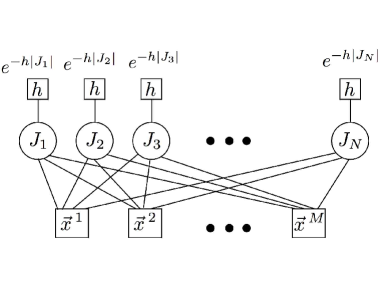
The belief propagation (BP) method, also known as Bethe-Peierls approximation, or cavity approach, in statistical physics, is exact on tree-shaped graphical models. As an approximate tool, it was therefore mostly used on sparse graphs Yedidia et al. (2001); Kschischang et al. (2001); Braunstein et al. (2005), where the influence of loops is expected to be not very strong. More recently, several applications to dense graphs have been successfully proposed Kabashima (2008); Uda and Kabashima (2005); Bickson et al. (2007); Braunstein and Zecchina (2005); Frey and Dueck (2007); Leone et al. (2007). Our problem can in fact be considered as a graphical problem over a fully connected bipartite factor graph, cf. Fig. 1, with $N$ vertices (variable nodes) representing the $N$ variables $J_{i}$, and $M$ vertices (factor nodes) representing the $M$ constraints (2). All pairs of these two vertex types are connected, since each constraint depends on all variables. In addition there are local fields on variables corresponding to the diluting term in Hamiltonian (5).

The BP algorithm provides a strategy for estimating marginal probability distributions. It works via iterative updates of messages, which are exchanged between variable and factor nodes. Let $\mu$ be one of the factor nodes and $i$ one of the variable nodes. We can introduce the following messages, which travel according to the direction indicated by the indices:

• $\rho_{\mu\rightarrow i}(J_{i})$ describes a weight imposed by constraint $\mu$ on the value $J_{i}$ of the coupling of variable $i$.

• $P_{i\rightarrow\mu}(J_{i})$ is the probability that variable $i$ takes value $J_{i}$ in the absence of the constraint set by factor node $\mu$.

The above-defined quantities satisfy the following set of self-consistent BP equations:

$$\rho_{\mu\rightarrow i}\left(J_{i}\right) = \sum_{\left\{J_{j}\right\}_{j\neq i}}\exp\left\{-\beta\Theta\left(-y^{\mu}\sum_{s=1}^{N}J_{s}x_{s}^{\mu}\right)\right\}\prod_{j\neq i}P_{j\rightarrow\mu}\left(J_{j}\right)$$ (17)

$$P_{i\rightarrow\mu}\left(J_{i}\right) = C_{i\to\mu}e^{-h|J_{i}|}\prod_{\nu\neq\mu}\rho_{\nu\rightarrow i}\left(J_{i}\right)$$ (18)

where $C_{i\to\mu}$ is a normalization constant. A more detailed derivation of the equations in the case of the perceptron without dilution can be found in Braunstein and Zecchina (2005), and in Braunstein et al. (2008) in the case of dilution.

In the algorithm both types of messages are initialized randomly, and the iteration proceeds via a random sequential update scheme. The algorithm stops when the convergence is reached, i.e. when the difference between each message at time $t$ and the corresponding one at time $t-1$ is less than a predefined threshold ($10^{-12}$ in all our simulations). The number of needed iterations depends on the particular problem and on the values settled for the parameters $\beta$ and $h$. However, we do not exceed a hundred of iterations in the simulations reported above.

Once all messages are evaluated, the desired marginal probability is given by the messages sent from all factor nodes and by the diluting field,

$$P_{i}(J_{i})=C_{i}e^{-h|J_{i}|}\prod_{\nu}\rho_{\nu\rightarrow i}\left(J_{i}\right)$$ (19)

where the $C_{i}$ are normalization constants which can be easily determined by tracing the unnormalized expression over the three values $J_{i}=0,\pm 1$.

Note that in the definition of messages (17) we still have a sum over $3^{N-1}$ configurations, but they enter in the expression only through a linear combination, which enables us to use again a Gaussian approximation Braunstein and Zecchina (2005). The sum over couplings is replaced by a single Gaussian integral, which can be performed explicitly:

$$\rho_{\mu\rightarrow i}\left(J_{i}\right) = \int_{-\infty}^{+\infty}\frac{dz_{\mu\rightarrow i}}{\sqrt{2\pi\sigma_{\mu\rightarrow i}^{2}}}\exp\left\{-\frac{\left(z_{\mu\rightarrow i}-\bar{z}_{\mu\rightarrow i}\right)^{2}}{2\sigma_{\mu\rightarrow i}^{2}}\right\}\exp\left\{-\beta\Theta\left(-y^{\mu}\left(z_{\mu\rightarrow i}+J_{i}x_{i}^{\mu}\right)\right)\right\}$$ (20)

$$= \frac{1+e^{-\beta}}{2}+\frac{1-e^{-\beta}}{2}\ {\rm erf}\left\{y^{\mu}\frac{\bar{z}_{\mu\rightarrow i}+J_{i}x_{i}^{\mu}}{\sqrt{2\sigma_{\mu\rightarrow i}^{2}}}\right\}$$ (21)

where $z_{\mu\rightarrow i}$ is a Gaussian variable with mean and variance,

$$\bar{z}_{\mu\rightarrow i} = \sum_{j\neq i}\langle J_{j}\rangle_{j\to\mu}\ x_{j}^{\mu}$$

$$\sigma_{\mu\rightarrow i}^{2} = \sum_{j\neq i}\left({\langle J}_{j}^{2}\rangle_{j\to\mu}\ -{\langle J}_{j}\rangle_{j\to\mu}^{2}\right){x_{j}^{\mu}}^{2}\ .$$ (22)

The averages $\langle\cdot\rangle_{j\to\mu}$ are performed over messages $P_{j\to\mu}(J_{j})$. In this way the complexity of Eq. (17) is reduced from ${\cal O}(3^{N})$ to ${\cal O}(N)$ and that of the overall iteration to ${\cal O}(MN)$ (The apparent complexity ${\cal O}(MN^{2})$ of updating $MN$ messages in time ${\cal O}(N)$ can be reduced to ${\cal O}(MN^{2})$ by a simple trick: The sums in Eqs. (22) can be calculated over all $j$ once for each $\mu$, so only the contribution of $i$ has to be removed in the update of $\rho_{\mu\to i}$ for each $i$. This allows to make the single update step in constant time). A precise estimate of the overall complexity of the algorithm would require to control the scaling of the number of iterations needed for convergence. A theoretical analysis of BP convergence times in a general setting (including the perceptron case) remains elusive. Some recent progress for the simpler matching problem can be found in Bayati et al. (2008).

The BP equations become feasible even for very large $N$ and $M$, and can therefore be applied to biological high-throughput data sets. Note that, even if the central limit theorem is meant to be valid in the limit of $N\rightarrow\infty$, in practice it works very well already for $N=4$ (where the exact computation is clearly feasible).

The Bethe entropy Yedidia et al. (2001) can be computed from marginals and messages:

$$S_{\rm Bethe} = -\sum_{\mu=1}^{M}\sum_{\vec{J}}P_{\mu}(\vec{J})\ln P_{\mu}(\vec{J})+(M-1)\sum_{i=1}^{N}\sum_{J_{i}=-1,0,1}P_{i}(J_{i})\ln P_{i}(J_{i})$$ (23)

$$= -\sum_{\mu=1}^{M}\ln C^{\mu}-\sum_{\mu=1}^{M}C^{\mu}\sum_{i=1}^{N}\sum_{J_{i}=-1,0,1}\rho_{\mu\rightarrow i}(J_{i})P_{i\rightarrow\mu}(J_{i})\ln P_{i\rightarrow\mu}(J_{i})+\beta\sum_{\mu=1}^{M}C^{\mu}E_{\mu}$$

$$+(M-1)\sum_{i=1}^{N}\sum_{J_{i}=-1,0,1}P_{i}(J_{i})\ln P_{i}(J_{i})$$

In the first line, we have used the distribution

$$P_{\mu}(\vec{J})=C^{\mu}\exp\left\{-\beta\Theta\left(-y^{\mu}\sum_{s=1}^{N}J_{s}x_{s}^{\mu}\right)\right\}\prod_{j=1}^{N}P_{j\to\mu}(J_{j})$$ (24)

which describes the influence of a single factor node by conserved marginal distributions. In the second line, we use the corresponding single sample energy $c^{\mu}E_{\mu}$ defined as

$$E_{\mu} = \sum_{\left\{J_{j}\right\}_{j\neq i}}\Theta\left(-y^{\mu}\sum_{s=1}^{N}J_{s}x_{s}^{\mu}\right)\exp\left\{-\beta\Theta\left(-y^{\mu}\sum_{s=1}^{N}J_{s}x_{s}^{\mu}\right)\right\}\prod_{j\neq i}P_{j\rightarrow\mu}\left(J_{j}\right)$$ (25)

$$= \frac{e^{-\beta}}{2}\left[1-{\rm erf}\left\{y^{\mu}\frac{\bar{z}_{\mu\rightarrow i}+J_{i}x_{i}^{\mu}}{\sqrt{2\sigma_{\mu\rightarrow i}^{2}}}\right\}\right]\ .$$

In writing the last expression we have used again the Gaussian approximation as in Eqs. (20-22).

Up to this point, the BP equations still depend on two undetermined parameters, namely the inverse temperature $\beta$ coupled to the data-given constraints, and the diluting field $h$. To implement the algorithm we have to define a strategy for fixing these free parameters:

• The diluting field $h$ is the conjugate variable of the number of effective link $N_{\mathrm{eff}}(\vec{J})$, so we can equivalently fix one of the two quantities. We decided to fix the number of effective links, and thus the size of the searched gene signature, and to choose $h$ accordingly. To find the correct value of $h$ we apply a cooling procedure, where after each interaction of the BP equations step we increase (resp. decrease) $h$ depending on whether the effective number of link is higher (resp. lower) than the desired value. Since the true number of relevant genes is an unknown quantity, the chosen value for $N_{\mathrm{eff}}(\vec{J})$ is, however, a free parameter. Practically, since the algorithm finds marginal probabilities and not a single configuration, we define the number of relevant links via its thermodynamic average:

  $$\langle N_{\mathrm{eff}}\rangle=\sum_{i=1}^{N}[1-P_{i}(0)]\ .$$ (26)

  Comparing results for different values of $\langle N_{\mathrm{eff}}\rangle$ we see that the algorithm is fairly robust, as will be seen in the following sections.

• The inverse temperature $\beta$ is again fixed by a cooling procedure starting from a low value and increasing it until one of the following two conditions is met: (i) the energy reaches a small enough value ($\beta\to\infty$ formally corresponds to zero energy), (ii) the entropy goes to zero (a signal for a freezing transition into a non-extensive number of coupling configurations at finite temperature). In this last case we use the marginals computed at the zero-entropy temperature.

The diluting field $h$ drives the system toward solutions of the desired average number of effective coupling $\langle N_{\mathrm{eff}}\rangle$. This is not yet enough for determining explicitly one signature of the desired size, since results are still of probabilistic nature. If we want to select, and use in our algorithm, only a desired number of genes, we have to couple the BP algorithm with the decimation procedure presented in Mézard et al. (2002); Mézard and Zecchina (2002):

1. Random initialization of messages.

2. Convergence of the BP Eqs. (17) and (18) at the correctly self-tuned values of $h$ and $\beta$.

3. Computation of marginal probability distributions using Eq. (19).

4. Setting to zero the coupling variable $J_{i}$ having the largest weight in zero (i.e., set $P_{i}(J_{i}=0)=1$ for this variable).

5. GOTO 2. Repeat until $N-N_{\mathrm{eff}}$ classification variables are set to zero.

Practically, this procedure turned out to be computationally much too expensive, so we opted for a faster variant of Step 4 of the decimation procedure: after each convergence step of the BP equations, we rank genes according to $P_{i}(0)$, and we set to zero an extensive part of couplings at the top of this ranking. The same procedure is iterated until we reach the desired number of non zero weights $J_{i}$.

III.2 A note on the centroids algorithm

It is interesting to compare the results of the BP algorithm with simpler, but widely applied techniques. The centroids algorithm is based on the notion of distance (Euclidean distance in $N$-dimensional space in this case) of a given pattern from the centers of mass of the two sets of patterns with annotations $y^{\mu}=1$ or $-1$. The algorithm works in the following way:

• Let $B_{z}\equiv\{\mu\,|\,y^{\mu}=z\}$, and $M_{z}=|B_{z}|$ the number of patterns with label $z$. Here we consider $z=\pm 1$ only, but the algorithm works equivalently for multiple classes. We compute the centers of mass (or centroids) $\vec{c}_{z}$ of the expression data with labels $y=z$:

  $$\vec{c}_{z}=\frac{1}{M_{z}}\sum_{\mu\in B_{z}}\vec{x}^{\mu}$$ (27)

• We assign the label $y^{0}=z$ to a new sample $\vec{x}\,^{0}$ if its distance from $\vec{c}_{z}$ is smaller than its distance from all other centroids,

  $$y^{0}=\underset{z}{\operatorname{argmin}}(||\vec{x}\,^{0}-\vec{c}_{z}||)\ ,$$ (28)

  where $||.||$ can be the Euclidean distance in $\mathbb{R}^{N}$ or, depending on the problem, any other meaningful notion of distance.

In order to take into account that only a subset of the genes is relevant (sparse signature), we rank genes $i=1,...,N$ according to the absolute value of their Pearson correlation $C_{i}$ with the output:

$$C_{i}=\frac{\frac{1}{M}\sum_{\mu=1}^{M}x_{i}^{\mu}y^{\mu}-\left(\frac{1}{M}\sum_{\mu=1}^{M}y^{\mu}\right)\left(\frac{1}{M}\sum_{\mu=1}^{M}x_{i}^{\mu}\right)}{\sqrt{1-\left(\frac{1}{M}\sum_{\mu=1}^{M}y^{\mu}\right)^{2}}\sqrt{\frac{1}{M}\sum_{\mu=1}^{M}{x_{i}^{\mu}}^{2}-\left(\frac{1}{M}\sum_{\mu=1}^{M}x_{i}^{\mu}\right)^{2}}}\ .$$ (29)

The $s$ highest scoring genes are selected as the signature, and the distance of the new pattern $\vec{x}\,^{0}$ from the centroids is computed taking into account only these genes, i.e. the full problem is projected onto the $s$-dimensional subspace of all genes. Since the signature size $s$ yielding the best classification is not known a priori, one has to consider the performance of the algorithm as a function of it.

Figure 2: Generalization error as a function of the signature size $s$ for artificial data generated according to Eqs. (30,31) with $N=600$ and $k_{1}=k_{2}=0.025$ (left and central panel) and according to the centroids rule with $k=6$ (right panel). In the left and right panel we have $M_{\mathrm{training}}=600$ ($\alpha=1$), in the central panel $M_{\mathrm{training}}=300$ ($\alpha=0.5$). In all the cases $M_{\mathrm{test}}=300$. The curves are averages over 50 different realizations of the training and test sets.

Figure 3: Precision-versus-recall curves for the teacher-student scenario. Results for the perceptron-like dataset in the case $\alpha=M_{\mathrm{training}}/N=1$ (left panel) and $\alpha=M_{\mathrm{training}}/N=0.5$ (central panel), and for the centroids-like dataset for $\alpha=M_{\mathrm{training}}/N=1$ (right panel). We display curves obtained from the BP algorithm with decimation (see text) for different values of the signature $s$. The curves derived from the Pearson correlation ranking used in the centroids algorithm are significantly lower than the BP ones in the perceptron-like dataset case. The same recall leads to lower precision in this case. In the centroids-like dataset case (displayed $s=600$), the curves for the two algorithms are comparable but BP continues to perform slightly better. Performance goes slightly down for smaller $s$ but stays comparable. In the left and right panel we have $M_{\mathrm{training}}=600$ ($\alpha=1$), in the central panel $M_{\mathrm{training}}=300$ ($\alpha=0.5$). In all the cases $M_{\mathrm{test}}=300$. The curves are averages over 50 different realizations of the training and test sets.

IV Test on artificially generated data

Before running the algorithm on micro-array data, it is useful to test it on artificial data generated by a controlled input-output relation. In the simulations reported here the $x_{i}^{\mu}$ are drawn independently from a normal distribution.

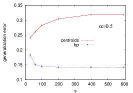
In order to compare the performance of the BP and the centroids algorithms, we label the random generated patterns according to two different rules, reflecting the perceptron and the centroids idea respectively.

IV.1 Description of the datasets.

In the first series of simulations, we draw the couplings $J_{i}^{0}$ from the following distribution:

$$P_{1}(J_{i}^{0})=(1-k_{1}-k_{2})\delta_{J_{i}^{0},0}+\frac{k_{1}}{2}[\delta_{J_{i}^{0},1}+\delta_{J_{i}^{0},-1}]+\frac{k_{2}}{2}[\delta_{J_{i}^{0},2}+\delta_{J_{i}^{0},-2}]\ .$$ (30)

We consider the case $k_{1}+k_{2}\ll 1$ in order to have a sparse gene signature, the expectation value of $N_{\rm eff}$ (defined as the number of non-zero entries of $\vec{J}\,^{0}$) equals $(k_{1}+k_{2})N$. Labels are determined according to a rule similar to the one used for BP inference,

$$y^{\mu}=\mathrm{sign}\left(\sum_{i=1}^{N}J_{i}^{0}x_{i}^{\mu}\right)\ .$$ (31)

If $k_{2}=0$ only $J_{i}^{0}=0,\pm 1$ exist, values $\pm 2$ are excluded. In this case the data are feasible under model if Eq. 2, and data can be learned at zero energy (no wrongly assigned labels by the inferred vector $\vec{J}$). The theoretical analysis presented in Braunstein et al. (2008) shows a phase-transition line in the plane $(\alpha,h)$, with $\alpha=M/N$. One phase, at low $\alpha$ and $h$, is paramagnetic. It perfectly memorizes the input-output relation given by the data, but there is no correspondence between the exponential number of possible coupling vectors and the data generating rule, the predictive properties for a new pattern $\vec{x}\,^{0}$ are poor. For higher $h$ and/or $\alpha$, the solution discontinuously jumps to a perfect retrieval of the input-output association vector $\vec{J}\,^{0}$. A particularly important point is that at sufficiently high diluting field $h$ perfect inference is possible at $\alpha$-values much lower than the critical threshold $\alpha_{c}$ for perfect inference at $h=0$.

In the case $k_{1,2}\neq 0$ the data are infeasible, since the structure of the data generator is richer than the one used for inference. Couplings of the data generator are allowed to take 5 values ({$\pm 2,\pm 1,0\}$), and inference tries to fit data just using ternary couplings ($\{\pm 1,0\}$).

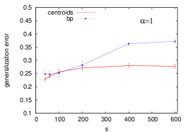
In the second series of simulations the patterns $\vec{x}\,^{\mu}$ are labeled according to their similarity to two vectors, $\vec{x}\,_{+}$ and $\vec{x}\,_{-}$, chosen as representative of the two classes. In order to take into account the sparsity of the relevant genes, we consider the variables $c_{i}=1$ if $i=1,\dots k$ and $c_{i}=0$ if $i=k+1,\dots N$, with $k\ll N$. We thus classify the patterns according to the restricted Euclidean distance:

$$y^{\mu}=\underset{z}{\operatorname{argmin}}\left(\sum_{i=1}^{N}c_{i}\sqrt{(x_{i}^{\mu}-x_{i,z})^{2}}\right)=\underset{z}{\operatorname{argmin}}\left(\sum_{i=1}^{k}\sqrt{(x_{i}^{\mu}-x_{i,z})^{2}}\right)\;\;\;\;\;z\in\{+,-\}\ .$$ (32)

IV.2 Results.

We investigate the goodness of the two classifier, in the two different situations described above, according to two different measures. First, we consider the generalization error. In this case patterns are divided into disjoint training and test sets. Learning is done on the training set, and the inferred input-output rule is tested against the test set. The generalization error is defined as the fraction of misclassified patterns in the test set. Results are shown in Fig. 2. For the first type of dataset (perceptron-like) one can appreciate how BP outperforms the simple centroids algorithm. In the second type of dataset (centroids-like), the centroids algorithm outperforms BP in the high signature cases but the two algorithms are comparable for low signatures.

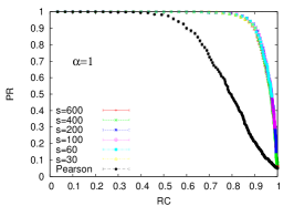
As a second test on the accuracy of BP, we use the fact that the data-generating signature is known. It can be compared directly to the inferred one, allowing to group genes into four classes: True positives (TP) are those genes which are contained in both signatures, i.e. genes which are correctly identified as being relevant by the inference algorithms. False positives (FP) are in the inferred signature, but they are not in the true one. In analogy we define true negatives (TN) as those which are in neither signature, and false negatives (FN) are those genes which are in the data generator, but they are not recognized by the algorithm. The recall RC (or sensitivity) and the precision PR (or specificity) are thus defined as:

$$RC=\frac{N_{TP}}{N_{TP}+N_{FN}}\ ,\ \ \ \ \ \ PR=\frac{N_{TP}}{N_{TP}+N_{FP}}\ .$$ (33)

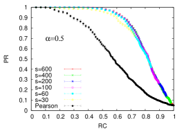
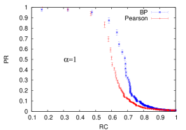
The recall $RC$ thus measure the fraction of correctly inferred genes in the signature, while precision $PR$ is the fraction of inferred couplings which are actually true ones. These two quantities are obviously competing: An algorithm that includes all genes into the signature has very low precision ($PR=\frac{N_{TP}}{N}$) but maximum recall ($RC=1$), while including only the genes with very strong signal into the signature may result in a good precision, but at the cost of a potentially poor recall. A perfect algorithm would have recall and precision both equal to one, so the interplay between both quantities is the relevant ”observable”. A curve precision-versus-recall can be constructed by ranking all genes according to their probability of having a non zero weight, and introducing different cutoffs in the ranking: In Fig. 3 we show the numerical results for the two datasets, while a more detailed theoretical analysis for the perceptron-like dataset can be found in Braunstein et al. (2008). We see that for the data generated by the perceptron like rule, BP actually performs considerably better than ranking by correlations, whereas results are comparably good in the case of the centroid-like generator.

V Test on tumor data

As stated in the introduction, a common problem of micro-array experiments is the small number of samples in the data set (from tens to hundreds) compared with the number (thousands) of monitored genes. Values of the parameter $\alpha=M/N$ in the considered data sets range from $\alpha=0.01$ to $\alpha=0.01$. In principle these values of $\alpha$ are below the threshold at which BP outperforms simple pairwise correlation based methods, at least on data artificially generated as described in the previous section and more extensively discussed in Braunstein et al. (2008). On the other hand, the simple ratio between the number of patterns and the number of genes might not be the relevant parameter on real data sets, due to the non trivial correlations between different patterns, and between genes. We first consider three data sets (leukemia, colon and prostate cancer), already analyzed in Dettling (2004) as benchmarks for other algorithmic strategies (e.g. BagBoost, Random Forest, Support Vector Machine, k-nearest neighbors, Diagonal Linear Discriminant Analysis). We further study a newer and larger data set on breast cancer from two different laboratories van de Vijver et al. (2002); van ’t Veer et al. (2002).

	$N$	$M$	Class A/B	$M_{\mathrm{training}}$	$M_{\mathrm{test}}$	NDP
Leukemia	3571	72	25/47	48	24	200
Prostate	6033	102	52/50	68	34	100
Colon	2000	62	40/22	42	20	200
Breast	6401	174	86/88	20-160	154-14	100

Table 1: In this table we display the number of probes $N$, the number of patterns $M$, the class composition of the data set Class A/B, the size of the training set $M_{\mathrm{training}}$, the size of the test set $M_{\mathrm{test}}$, and the number of different partitions NDP (see text) for each of the data set analyzed.

V.1 Description of the data sets

We have analyzed four different data sets of cancer tissues:

• Leukemia: It consists of 72 samples of two subtypes of leukemia – 25 samples of acute myeloid leukemia (Class A) and 47 samples of acute lymphoblastic leukemia (Class B) – measured over 3571 genetic probes Golub et al. (1999).

• Prostate It consists of 102 samples – 52 from prostate tumor tissues (Class A) and 50 from normal prostate tissues (Class B) – measured over 6033 genetic probes Singh et al. (2002).

• Colon: It consists of 62 samples – 40 from colon adenocarcinoma tissues (Class A) and 22 from normal colon tissues (Class B) – measured over 2000 genetic probes Alon et al. (1999).

• Breast: The data set we have analyzed is the union of two different experiments presented in van de Vijver et al. (2002); van ’t Veer et al. (2002): it contains 311 samples measured over 24496 probes. We labeled the samples according to the following criterion: a metastasis event occurred in the first 5 years after the appearance of the tumor (Class P [poor prognosis]), the remaining samples did not develop a metastasis in this time window and were labeled as Class G (good prognosis). In order to reduce the noise we removed all probes with nearly constant expression values across the data set. More specifically a probe is included in the data set if at least one of the of the following two conditions is met: (i) its variance is larger than 0.1, (ii) in at least ten samples its expression value is outside the window (-0.3,0.3). Eventually we ended up with 6401 probes. We further notice that the number of elements in Class P (86) is much smaller than those in Class G (225). Since a major aim in this context is to correctly classify all members of Class P (those developing metastasis) and not to misclassify them as Class G cases, a larger influence of class P data is needed. To obtain a more balanced dataset, we therefore randomly removed 137 elements from Class G and we end up with a set of 174 patients.

In Tab. 1 we resume the details of the data sets.

V.2 Results

Figure 4: Generalization error as a function of $N_{\mathrm{eff}}$ in the colon, prostate, and leukemia data set.

For each data set we construct different realizations of the training and test sets by randomly permuting the $M$ samples. The first $M_{\mathrm{training}}$ patterns will be the training set and the remaining $M_{\mathrm{test}}=M-M_{\mathrm{training}}$ patterns will be used as test set. In this way we are able to obtain results, which are not dependent on a single specific arbitrary partitioning of the patterns into training and test sets, and to attribute statistical errors to measured observables. In the last three columns of Tab. 1 we give the actual values of $M_{\mathrm{training}}$, $M_{\mathrm{test}}$, and the number of different partitions for each of the data sets.

In all data sets discussed here, we have run BP starting at finite temperature and using the cooling scheme described in Sec. III.1, which reached zero temperature. Running the algorithm at various fixed finite temperatures, we observed the generalization error to decrease monotonously with temperature, and to saturate at low temperature. Here we present directly the zero-temperature results obtained using cooling.

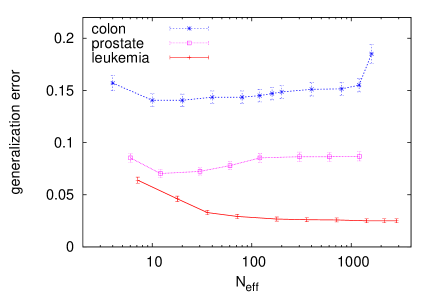
For the first three data sets (Leukemia, Prostate, and Colon) we first run BP on the entire probe-set with the diluting field $h$ defined in Eq. (6). We show in Fig. 4 the generalization error for the three data set as a function of $N_{\mathrm{eff}}$, which, as already explained in Sec. III.1, can be fixed by tuning the field $h$.

In Fig. 4 two different scenarios emerge: the colon and prostate curves display a minimum generalization error at a relatively low value of $N_{\mathrm{eff}}\sim 10$, while the leukemia curve is monotonously decreasing. This seems to indicate the presence of a small set of probes relevant for the classification in the prostate and colon case, while in the leukemia data set it seems that all probes are relevant for the classification.

Let us recall that a given $N_{\mathrm{eff}}$ does not necessarily indicate the actual size of the set of relevant probes. This would be the case only when all probabilities $P_{i}(J)$ were completely polarized (i.e. $P_{i}(0)$ is either 0 or 1). Upon direct inspection of our BP results it turns out that this is not the case. No clear threshold is shown on the marginals $P_{i}(0)$. The dilution thus seems to be an effective strategy to attribute differential weights to the probes, but it is not clear how to use it to select a relevant signature in the data set. A possible way is to implement a decimation procedure as explained in Sec. III.1, in order to test the performance of the algorithm on a restricted and selected set of probes (signatures) of different size.

Domany et al. in Ein-Dor et al. (2006) studied the stability of different signatures as a function of the number of samples used for learning. They interestingly noted that the small overlap between different signatures is not only due to the different classification strategies used by different groups, but in particular resulting from the small number of available cases. Such a lack of robustness emerges even when using the same algorithm on data generated with the same probabilistic framework Ein-Dor et al. (2006). We have investigated how stable are the lists obtained with our decimation procedure. It turns out that an analogous phenomenon of instability occurs in our lists. We observed very few genes appearing in all lists: the actual numbers differs among the different data sets but it ranges from 10% in the case of Leukemia, to 0.02% in the case of prostate tissues, where however the number of relevant genes seems to be very small as we will see in the following.

Figure 5: Generalization error computed with Centroids (blue line) and Belief Propagation (red line), as a function of the signature size s, shown with a logarithmic scale on the x axes. We display results for leukemia (left panel), prostate (central panel), and colon (right panel).

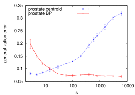
To understand how BP compares with simpler algorithmic strategies, we used the centroids method selecting signatures of the same size. The results for the first three data set are displayed in Fig. 5. The curve for Leukemia displays a monotonously decreasing profile in agreement with what we have obtained fixing $N_{\mathrm{eff}}$ shown in Fig. 4. This seems to indicate that no signature can be defined in this case. The generalization error obtained with the centroids algorithm is slightly worse then that of BP. The Prostate case displays dramatic difference in the two algorithms: from the BP point of view the curve displays a plateau of minimal generalization error for signature larger than 100, at odd with what obtained fixing $N_{\mathrm{eff}}$ where a minimum is present around $N_{\mathrm{eff}}=10$. Also in this case it seems difficult to determine a clear signature in the data set. Centroids behaves in the opposite way displaying a monotonously increasing function with minimal generalization error at values of the signature lower than 10. The optimal generalization error achieved by the two algorithm in this case is compatible. The Colon case is analogous to that of Prostate from the BP point of view (the minimum generalization error is obtained for $N_{\mathrm{eff}}=10$ but for $s=400$), while centroids seems to be rather insensitive to signature size in the whole interval analyzed. In this case BP shows an overall better generalization ability. The discrepancy between the values of the signature $s$ and of the $N_{\mathrm{eff}}$ for which the generalization error is minimum, comes from the not unique set of possible relevant genes. While the algorithm is able to select genes which are relevant and weight them adequately ($N_{\mathrm{eff}}$ small), it is not able to define a single clear signature which alone is sufficient for the classification. This implies that, in the decimation procedure, a much higher number of genes, even if with small weight, is necessary to achieve a good predictive ability (so that the minimum generalization error is reached for signatures $s$ much bigger than the probabilistic expectation given by $N_{\mathrm{eff}}$). It is worth pointing out that the fact that BP behaves worse for very small sizes, is already present in the case artificial data Fig. 2.

The best generalization errors of both BP and centroids are displayed in Tab. 2 compared with the results presented by Dettling in Dettling (2004) where no statistical error was associated with measures. We see that BP outperforms 4 out of 6 other algorithms on all three data sets, the other two algorithms perform better on a single data set each.

	BP	centroids	BagBoost	RanFor	SVM	kNN	DLDA
Leukemia	0.025(2)	0.029(2)	0.0408	0.025	0.035	0.0383	0.0292
Prostate	0.070(4)	0.071(4)	0.0753	0.0788	0.0682	0.1059	0.1418
Colon	0.140(6)	0.156(4)	0.1610	0.1543	0.1667	0.1638	0.1286

Table 2: In this table we compare the generalization errors of our method (first column) against centroids, BagBoost, RanFor, SVM, kNN, and DLDA presented in Dettling (2004).

In the breast-cancer case, we consider first the generalization error for various sizes of the training set ($M_{\rm training}=20,...,160$). The relatively large balanced data set containing 174 patients allows for the direct analysis of sample sizes ranging over almost a full order of magnitude. The results are presented in the left panel of Fig. 6, each point is averaged over 50 random selections of the training set. We observe a strong monotonous decrease of the generalization error. This is a very encouraging sign and should motivate for collecting larger data sets. The generalization error of 30% obtained for $M_{\rm training}=80$ is compatible with the one ($31\%$) reported in Michiels and Koscielny (2005).

However, in the breast cancer set we can go into more detail: The generalization error treats good and poor cases (Classes G/P) in the same way. Indeed, one of the open challenges in breast cancer treatment is to recognize the correct cancer sub-type at the earliest possible stage of disease, indicating, e.g., the possible sensitivity of the cancer to chemotherapy. In the present case, it is strongly preferable to erroneously include a Class G patient into Class P than vice versa; it has to be avoided to predict the absence of metastasis for a patient who actually develops one, and possibly not to provide the necessary medical treatment to such a patient.

We therefore introduce four different subclasses:

1. patients in Class G (no metastasis) correctly classified as Class G, their number is called $M_{\rm GG}$;

2. patients in Class P (metastasis) misclassified as Class G, their number is called $M_{\rm PG}$;

3. patients in Class G (no metastasis) misclassified as Class P, their number is called $M_{\rm GP}$;

4. patients in Class P (metastasis) correctly classified as Class P, their number is called $M_{\rm PP}$.

As said before, our primary aim is to classify correctly Class P patients. The fraction $M_{\rm PG}/(M_{\rm PP}+M_{\rm PG})$ of misclassified Class P patients has to be kept as small as possible; we refer to it as the poor error fraction (PEF). Once this is kept small, we also would like to recognize correctly as many Class G patients as possible. The corresponding fraction in the total Class G sample is $M_{\rm GG}/(M_{\rm GG}+M_{\rm GP})$, we refer to it as the good prediction fraction (GPF).

The GPF vs. PEF curve for a perfect classifier would be constantly equal to zero for the full GPF range, while a random classifier would produce a curve PEF=GPF. Here we want to characterize the relation of these two competing quantities (a constant prediction as P would have PEF=GPF=0, whereas a constant prediction G would have PEF=GPF=1), keeping however in mind that we want to keep the PEF low. The full curve is obtained done by changing the threshold $\tau$ defined in Eq. (2) of the inferred classifier.

The result is displayed in the right panel of Fig. 6 for training sets of size $M_{\rm training}=100,\,160$. For each possible PEF value we have averaged the curve over 50 random balanced partitionings of our data into training / test sets. When training with 100 samples, we have 37 points corresponding to the possible numbers of misclassified Class P patients (0 to 36). When training with 160 samples, this number reduced to 8 points. Note that the finding that the curve for larger training sets is located right of the other curve is consistent with the observation done in the left panel of Fig. 6: Larger training sets lead to better results. It is particularly striking that the PEF starts to grow much later, the GPF at zero PEF grows from about 10% to about 40%. Again we see that larger data sets should be collected for developing more precise prognostic tools.

In order to compare our result with that of van de Vijver et al. (2002), we measured the value of the GPF corresponding to an average PEF value around $0.07$. This can be obtained by averaging over cases with $M_{\rm PG}$ being at most one. In this case we obtained a PEF of 0.076(1) and a GPF of 0.50(2). These values are comparable to van de Vijver et al. (2002) where a PEF=0.071 and GPF=0.53 are reported for a set of 180 patients and a leave-one-out procedure ($M_{\rm training}=M-1$).

In conclusion, for the breast cancer dataset, we obtain results comparable with state of the art studies, and we find a not saturated increase of performance with growing training set size.

Figure 6: Results for the breast-cancer dataset. Generalization error as a function of the training set size (left) and PEF (fraction of Class P patients classified as G) vs. GPF (fraction of correctly classified Class G patients).

VI Conclusion and Perspectives

In this work we introduced and analyzed a message passing algorithm for the problem of classification and applied it to genome-wide expression patterns of cancer tissues. The aim of the algorithm is twofold: on one hand one would like to get a reliable classifier, on the other hand one wants to base this result on a minimal set of discriminating genes. This additional requirement of parsimony is based on the biological intuition that, as long as the expression level is concerned, only a relatively small subset of genes is actually significant for the development of the disease. Furthermore the possibility of identifying a meaningful (possibly small) signature of the disease will help the classification in two ways: (i) computationally, the dimensional reduction of the patterns makes the classification less prone to over-fitting, (ii) experimentally, specific targeted gene-chip scanning could improve early stage cancer diagnostic (e.g. in the case of breast-cancer).

The performance of our algorithm is found to be slightly better, although comparable with the one of other state-of-the-art classification techniques. Using three different data sets, the BP performed better than 4 out of 6 algorithms on all data sets, and better than the other 2 algorithms on two out of the three data sets. The obtained results are compatible with the following theoretical intuition: The sparse quality (experimental and biological noise) and quantity (few expression patterns) of available data does not allow to extract substantially more information than the one seen also by simple algorithms. From this point of view the situation will improve in the near future since gene-chip technologies are becoming more and more diffused, and the emergence of new array technologies based on longer oligo-nucleotides should reduce the experimental noise of the expression measurements. This ongoing technological revolution calls for the development of sophisticated global classification techniques which are able to unravel, e.g., combinatorial control.

Another line of development in tumor detection is the integration of different sources of information. From this point of view SNPs (Single Nucleotide Polymorphism) appear to be the most promising high-throughput genome-wide technology.

VII Acknowledgments

We thank Alfredo Braunstein, Yoshiyuki Kabashima, Michele Leone, and Riccardo Zecchina for very interesting discussion on the problem of inference and methodological aspects of message passing algorithms. We also thank Enzo Medico for pointing out the Breast Cancer data set, and the centroids algorithm.

References

- Bair and Tibshirani (2004) E. Bair and R. Tibshirani, PLoS Biology 2, e108+ (2004), URL http://dx.doi.org/10.1371%2Fjournal.pbio.0020108.
- Beer et al. (2002) D. G. Beer, S. L.R., C.-C. Huang, T. J. Giordano, A. M. Levin, D. E. Misek, C. G. Lin, L., T. G. Gharib, D. G. Thomas, M. L. Lizyness, et al., Nat. Med. 8, 816 (2002), URL http://dx.doi.org/10.1038/nm733.
- Bhattacharjee et al. (2001) A. Bhattacharjee, W. G. Richards, J. Staunton, C. Li, S. Monti, P. Vasa, C. Ladd, J. Beheshti, R. Bueno, M. Gillette, et al., Proceedings of the National Academy of Sciences 98, 13790 (2001), eprint http://www.pnas.org/cgi/reprint/98/24/13790.pdf, URL http://www.pnas.org/cgi/content/abstract/98/24/13790.
- Ramaswamy et al. (2003) S. Ramaswamy, K. N. Ross, E. S. Lander, and T. R. Golub, Nat. Genet. 33, 49 (2003), URL http://dx.doi.org/10.1038/ng1060.
- Guyon and Elisseeff (2003) I. Guyon and A. Elisseeff, Journal of Machine Learning Research 3, 1157 (2003).
- Guyon et al. (2006) I. Guyon, S. Gunn, M. Nikravesh, and L. Zadeh, Feature Extraction: Foundations and Applications (Springer-Verlag, 2006).
- Ein-Dor et al. (2006) L. Ein-Dor, O. Zuk, and E. Domany, Proc Natl Acad Sci U S A 103, 5923 (2006), ISSN 0027-8424, URL http://dx.doi.org/10.1073/pnas.0601231103.
- Jain et al. (1999) A. K. Jain, M. N. Murty, and P. J. Flynn, ACM Computing Surveys 31, 264 (1999), URL citeseer.ist.psu.edu/jain99data.html.
- Duda et al. (2000) R. O. Duda, P. E. Hart, and D. G. Stork, Pattern Classification (Wiley-Interscience Publication, 2000).
- Braunstein et al. (2008) A. Braunstein, A. Pagnani, M. Weigt, and R. Zecchina, J. Stat. Mech. P12001 (2008).
- Yedidia et al. (2001) J. S. Yedidia, W. Freeman, and Y. Weiss, in Advances in Neural Information Processing Systems (NIPS) 13, Denver, CO, edited by M. press (2001), pp. 772–778.
- Dettling (2004) M. Dettling, Bioinformatics 20, 3583 (2004), ISSN 1367-4803, URL http://dx.doi.org/10.1093/bioinformatics/bth447.
- van de Vijver et al. (2002) M. J. van de Vijver, Y. D. He, L. J. van’t Veer, H. Dai, A. A. Hart, D. W. Voskuil, G. J. Schreiber, J. L. Peterse, C. Roberts, M. J. Marton, et al., N. Engl. J. Med. 347, 1999 (2002), ISSN 1533-4406, URL http://dx.doi.org/10.1056/NEJMoa021967.
- van ’t Veer et al. (2002) L. J. van ’t Veer, H. Dai, M. J. van de Vijver, Y. D. He, A. A. Hart, M. Mao, H. L. Peterse, K. van der Kooy, M. J. Marton, A. T. Witteveen, et al., Nature 415, 530 (2002), ISSN 0028-0836, URL http://dx.doi.org/10.1038/415530a.
- Uda and Kabashima (2005) S. Uda and Y. Kabashima, J. Phys. Soc. Jpn. 74, 2233 (2005), eprint cond-mat/0502051.
- Clark and Boswell (2001) P. Clark and R. Boswell, in Proceedings of the 5th European Working Session on Learning (EWSL-91), edited by Springer-Verlag (2001), pp. 151–163.
- Hertz et al. (1991) J. Hertz, A. Krogh, and R. G. Palmer, Introduction to the Theory of Neural Computation (Addison-Wesley Publishing Company, Inc., Redwood City, CA, 1991).
- Braunstein and Zecchina (2005) A. Braunstein and R. Zecchina, Phys. Rev. Lett. 96, 030201 (2005), eprint cond-mat/0511159.
- Mackay (2002) D. J. C. Mackay, Information Theory, Inference & Learning Algorithms (Cambridge University Press, 2002), ISBN 0521642981, URL http://www.amazon.ca/exec/obidos/redirect?tag=citeulike09-20%&path=ASIN/0521642981.
- Kschischang et al. (2001) F. R. Kschischang, B. J. Frey, and H. A. Loeliger, Information Theory, IEEE Transactions on 47, 498 (2001), URL http://ieeexplore.ieee.org/xpls/abs_all.jsp?arnumber=910572.
- Braunstein et al. (2005) A. Braunstein, M. Mezard, and R. Zecchina, Random Struct. Algorithms 27, 201 (2005), URL http://dblp.uni-trier.de/db/journals/rsa/rsa27.html#Braunstei%nMZ05.
- Kabashima (2008) Y. Kabashima, Journal of Physics: Conference Series 95, 012001 (13pp) (2008), URL http://stacks.iop.org/1742-6596/95/012001.
- Bickson et al. (2007) D. Bickson, D. Dolev, O. Shental, P. H. Siegel, and J. K. Wolf (2007).
- Frey and Dueck (2007) B. J. Frey and D. Dueck, Science 315, 972 (2007), eprint http://www.sciencemag.org/cgi/reprint/315/5814/972.pdf, URL http://www.sciencemag.org/cgi/content/abstract/315/5814/972.
- Leone et al. (2007) M. Leone, Sumedha, and M. Weigt, Bioinformatics 23, 2708 (2007), eprint http://bioinformatics.oxfordjournals.org/cgi/reprint/23/20/2708.pdf, URL http://bioinformatics.oxfordjournals.org/cgi/content/abstract%/23/20/2708.
- Bayati et al. (2008) M. Bayati, C. Borgs, J. Chayes, and R. Zecchina, Journal of Statistical Mechanics: Theory and Experiment 2008, L06001 (10pp) (2008), URL http://stacks.iop.org/1742-5468/2008/L06001.
- Mézard et al. (2002) M. Mézard, G. Parisi, and R. Zecchina, Science 297, 812 (2002), URL http://aps.arxiv.org/pdf/0707.1295.
- Mézard and Zecchina (2002) M. Mézard and R. Zecchina, Phys. Rev. E 66, 056126 (2002), URL http://link.aps.org/abstract/PRE/v66/e056126.
- Golub et al. (1999) T. Golub, D. Slonim, P. Tamayo, C. Huard, M. Gaasenbeek, J. Mesirov, H. Coller, M. Loh, J. Downing, M. Caligiuri, et al., Science 286, 531 (1999).
- Singh et al. (2002) D. Singh, P. Febbo, K. Ross, D. Jackson, J. Manola, C. Ladd, P. Tamayo, A. Renshaw, A. D’Amico, J. Richie, et al., Cancer Cell 1, 203 (2002).
- Alon et al. (1999) A. Alon, N. Barkai, D. Notterman, K. Gish, S. Ybarra, D. Mack, and A. Levine, Proc. Natl. Acad. Sci. USA 96, 6745 (1999).
- Michiels and Koscielny (2005) S. Michiels and S. Koscielny, Lancet pp. 488–492 (2005).