EXOFIT: Bayesian Estimation of Orbital Parameters of Extrasolar Planets

Abstract

We introduce EXOFIT, a Bayesian tool for estimating orbital parameters of extra-solar planets from radial velocity measurements. EXOFIT can search for either one or two planets at present. EXOFIT employs Markov Chain Monte Carlo method implemented in an object oriented manner. As an example we re-analyze the orbital solution of HD155358 and the results are compared with that of the published orbital parameters. In order to check the agreement of the EXOFIT orbital parameters with the published ones we examined radial velocity data of 30 stars taken randomly from www.exoplanet.eu. We show that while orbital periods agree in both methods, EXOFIT prefers lower eccentricity solutions for planets with higher ($e\geq 0.5$) orbital eccentricities.

Astrophysics Group, Cavendish Laboratory, JJ Thomson Avenue, Cambridge CB3 0HE, UK

Department of Physics and Astronomy, University College, Gower Street, London WC1E 6BT, UK

1. Introduction

More than a decade of extensive search for extra-solar planets has resulted in nearly 300 planets. Majority of the contribution to the extra-solar planet count comes from radial velocity method. Radial velocity data is traditionally analyzed first by a periodogram (Lomb 1973; Scargle 1982) for the orbital period and then for the other orbital parameters using conventional optimization methods. Bayesian methods for the estimation of orbital parameters of extra-solar planets were introduced by Gregory (2005a) and Ford (2005). Their work shows that these methods provide us a framework to tackle the problems associated with the traditional methods in a transparent and robust manner. EXOFIT of Balan & Lahav (2008) is the first publicly available package for Bayesian estimation orbital parameters from radial velocity measurements. In this article we discuss the application of EXOFIT to the radial velocity data of HD155358 and compare our results with the published orbital solution (Cochran et al. 2007). We also show, by analyzing a randomly selected sample of radial velocity data from www.exoplanet.eu that EXOFIT disagrees with the published orbital eccentricities in many instances while the orbital periods from EXOFIT matches closely with the published ones.

The rest of the article is organized as follows. In Section 2. we give a brief introduction to radial velocity modeling. Section 3. describes Bayesian approach to parameter estimation. EXOFIT is introduced in Section 4. and its application to the radial velocity data is discussed in section 5.. Section 6. explains the analysis of radial velocity data of a sample of stars taken form www.exoplanet.eu using EXOFIT. We conclude this article in Section 7. and provide an outline on planned work.

2. Modeling of Radial Velocity Data

Radial velocity data consists of a set of measured radial velocity entries, corresponding time of observation and the uncertainty in each measurement. Observed radial velocity data is modeled by the equation (Gregory 2005a)

$$d_{i}=\nu_{i}+\epsilon_{i}+\delta,$$ (1)

where $d_{i}$ is the measured radial velocity data for the $i$th instant of time $t_{i}$, $\nu_{i}$ is true radial velocity of the star, $\epsilon_{i}$ is the measurement error assigned by the observer and $\delta$ represents any unknown noise present (e.g., signal from another planet) in the data. For a statistician, $\delta$ is a nuisance parameter. The true radial velocity can be simulated using a mathematical model. Disregarding any interactions between planets, the radial velocity of a star for a typical $n$-planet model can be approximately written as a linear combination of $n$ single planet radial velocities. Thus,

$$v=V-\sum_{i=1}^{n}K_{i}\big{(}\sin(f_{i}+\varpi_{i})+e_{i}\,\sin\varpi_{i}\big{)},$$ (2)

where $V,K,f,e,w$ represent the systematic velocity, amplitude, true anomaly, eccentricity and the longitude of periastron respectively. For the full formalism see the User’s Guide to EXOFIT.

3. Bayesian Parameter Estimation

Bayesian paradigm has its origins in an article published posthumously by Rev. Thomas Bayes in 1763. Since then the theorem has played a central part in probabilistic inference. For latest examples in cosmology see Feroz & Hobson (2008) and Lewis & Bridle (2002). Bayesian methods for the estimation of orbital parameters of extra-solar planets were introduced by Gregory (2005a) and Ford (2005) and their research show that this approach has an edge over the traditional methods when dealing with for e.g., highly eccentric orbits. These methods also provide a straight forward way of dealing with nuisance parameters and a robust way of estimating uncertainties associated with the estimates of orbital parameters.

Bayes’ theorem for a set of parameters $\mathbf{\Theta}$ in model $H$ and data $\mathbf{D}$ can be written as,

$$\Pr(\mathbf{\Theta}|\mathbf{D},H)=\frac{\Pr(\mathbf{D}|\mathbf{\Theta},H)\Pr(\mathbf{\Theta}|H)}{\Pr(\mathbf{D}|H)}.$$ (3)

In the above equation $\Pr(\mathbf{\Theta}|\mathbf{D},H)$ is the posterior probability distribution of parameters, $\Pr(\mathbf{D}|\mathbf{\Theta},H)$ is the likelihood of the data, $\Pr(\mathbf{\Theta}|H)$ represents the prior probability distribution of the parameters and $\Pr(\mathbf{D}|H)$ is called the Bayesian evidence. For parameter estimation problems we could simply write the above equation as

$$\Pr(\mathbf{\Theta}|\mathbf{D},H)\propto\Pr(\mathbf{D}|\mathbf{\Theta},H)\Pr(\mathbf{\Theta}|H)$$ (4)

Computing the right hand side of Equation 4 is the central point of any Bayesian parameter estimation . Analytical solutions can be derived for some special cases. However, in general we use numerical methods to compute the posterior distribution. Although many approximation methods exist, this area is dominated by Markov Chain Monte Carlo (MCMC) and other sampling methods. These rely on the a random walk through the parameter space and make use of the fact that posterior density is proportional to the number of points visited in the volume considered. We calculate the marginal posterior distribution of each parameter by simple plotting a histogram of the final set of samples.

Bayesian modeling of the problem consists of defining each of the components mentioned in Equation 4. This will be discussed from the context of estimation of orbital parameters when we apply EXOFIT to the published radial velocity data of HD155358 in Section 5..

4. EXOFIT

EXOFIT is an easy to use documented software for estimating the orbital parameters from radial velocity measurements and it is freely available. It is based on Bayesian MCMC method and is implemented in an object oriented framework in C++. It can be easily extended to analyze the radial velocity data of more than two planets as well as data from transit photometry. Output of EXOFIT is a set of posterior samples. These can be analyzed using any standard statistical software. This explained in User’s Guide which can be download from EXOFIT website. We also provide sample script for R statistical environment to analyze posterior samples. Improved parameterization for the problem and novel sampling techniques for EXOFIT are under development.

5. Application to Radial Velocity Data of HD155358

In this section we develop a Bayesian model for the parameter estimation and apply EXOFIT to extract the orbital parameters of the companions of HD155358. We start by defining the likelihood of the data. As mentioned in Section 2. we assume that the data consists of true radial velocity and some noise. The component of noise arising from the known measurement errors $\epsilon_{i}$ is assumed to be normally distributed with standard deviation $\sigma_{i}$ for the $i$th entry in the data. The probability distribution for the unaccounted noise component $\delta$ is chosen to a Gaussian distribution with finite variance $s^{2}$. Therefore, the distribution of the combination $\epsilon_{i}+\delta$ can be considered as a Gaussian with a variance of $\sigma_{i}^{2}+s^{2}$.

Assuming each measurement error $\epsilon_{i}$ to be independent and since they follow a Gaussian distribution, the likelihood of data can be written as a product $N$ Gaussians(Gregory 2005a) where $N$ is the number of entries in the data. Therefore,

$$\Pr(\mathbf{D}|\mathbf{\Theta},H)=A\,\exp\Biggl{[}-\sum_{i=1}^{N}\frac{(d_{i}-v_{i})^{2}}{2(\sigma_{i}^{2}+s^{2})}\Biggr{]}\,,$$ (5)

where

$$A=(2\pi)^{-N/2}\Biggl{[}\prod_{i=1}^{N}\big{(}\sigma_{i}^{2}+s^{2}\big{)}^{-1/2}\Biggr{]}\,.$$ (6)

Thus, our parameter space is $\{V,T_{1},K_{1},e_{1},w_{1},\chi_{1},T_{2},K_{2},e_{2},w_{2},\chi_{2},s\}$, first 11 from the mathematical model and last one representing the nuisance parameter $\delta$. The parameter is $\chi$ is defined for computational purposes and marks the periastron passage time as function period $T$. For more details please consult EXOFIT User’s Guide.

Table 1, taken from Balan & Lahav (2008) gives the prior probability distributions of each parameter in the model. These priors are chosen in such a way that they allow likelihood term in the Equation 4 to dominate the posterior distribution and thus ensuring inference to be drawn from the observed data.

Table 1.: The assumed prior distribution of orbital parameters and their boundaries for a 2-planet model.

Para.	Prior	Mathematical Form	Min	Max
$V(ms^{-1})$	Uniform	$\frac{1}{V_{max}-V_{min}}$	-2000	2000
$T_{1}(days)$	Jeffreys	$\frac{1}{T_{1}\,\ln\Big{(}\frac{T_{1\,max}}{T_{1\,min}}\Big{)}}$	0.2	15000
$K_{1}(ms^{-1})$	Mod. Jeffreys	$\frac{(K_{1}+K_{1\,0})^{-1}}{\ln\big{(}\frac{K_{1\,0}+K_{1\,max}}{K_{1\,0}}\big{)}}$	0.0	2000
$e_{1}$	Uniform	1	0	1
$\varpi_{1}$	Uniform	$\frac{1}{2\pi}$	0	$2\pi$
$\chi_{1}$	Uniform	1	0	1
$T_{2}(days)$	Jeffreys	$\frac{1}{T_{2}\,\ln\Big{(}\frac{T_{2\,max}}{T_{2\,min}}\Big{)}}$	0.2	15000
$K_{2}(ms^{-1})$	Mod. Jeffreys	$\frac{(K_{2}+K_{2\,0})^{-1}}{\ln\big{(}\frac{K_{2\,0}+K_{2\,max}}{K_{2\,0}}\big{)}}$	0.0	2000
$e_{2}$	Uniform	1	0	1
$\varpi_{2}$	Uniform	$\frac{1}{2\pi}$	0	$2\pi$
$\chi_{2}$	Uniform	1	0	1
$s(ms^{-1})$	Mod. Jeffreys	$\frac{(s+s_{0})^{-1}}{\ln\big{(}\frac{s_{0}+s_{max}}{s_{0}}\big{)}}$	0	$2000$

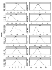
Application of EXOFIT revealed the posterior distribution of planets as given in Figure 1(a) and the corresponding radial velocity curve is shown in Figure 1(b). We compare our results to the published results by (Cochran et al. 2007) in Table 2. Although our results looks similar, we notice a noise factor($s$) of $5.43\,ms^{-1}$ which indicates the presence of an additional signal in the data. We did look for a third planet in the system, but our results were inconclusive. This issue can be settled if we have more observations down the line.

(a) Marginal posterior destributions

(b) Radial velocity curve

Figure 1.: Marginal postrior distribuotions of orbital orbital parameters of the companions to HD155358 are shown in the left panel. Right panel shows the corresponding radial velocity curve for HD155358.

Table 2.: A table showing the summary of the posterior distribution of orbital parameters extracted with EXOFIT 2-planet model and the published orbital solution by Cochran et al. (2007). Columns 2, 3 and 4 show the posterior mean (and standard deviation), median (and 25% and 75% quantiles) and the maximum a posteriori, i.e. posterior mode (and 68.3% highest density regions) respectively. Mass of the star was assumed to be $0.87M_{\oplus}$.

Parameters	EXOFIT(Mean)	EXOFIT(Median)	EXOFIT(Mode)	Cochran et al.
$V(ms^{-1})$	$11.09\pm 1.37$	$11.11_{-0.91}^{+0.91}$	$11.23_{-1.32}^{+1.17}$
$T_{1}(days)$	$195.22\pm 0.91$	$195.20_{-0.63}^{+0.64}$	$195.17_{-0.84}^{+0.87}$	$195\pm 1.1$
$K_{1}(ms^{-1})$	$33.56\pm 2.22$	$33.59_{-1.55}^{+1.48}$	$33.58_{-2.02}^{+2.07}$	$34.6\pm 3$
$e_{1}$	$0.13\pm 0.04$	$0.13_{-0.03}^{+0.03}$	$0.13_{-0.04}^{+0.03}$	$0.112\pm 0.037$
$\varpi_{1}(degrees)$	$160.78\pm 19.73$	$160.46_{-12.77}^{+12.82}$	$158.20_{-15.33}^{+19.30}$	$162\pm 20$
$\chi_{1}$	$0.38\pm 0.07$	$0.38_{-0.05}^{+0.05}$	$0.38_{-0.07}^{+0.06}$
$T_{2}(days)$	$537.05\pm 24.00$	$532.15_{-13.84}^{+22.78}$	$519.77_{-13.46}^{+29.19}$	$530.3\pm 27.2$
$K_{2}(ms^{-1})$	$14.40\pm 1.68$	$14.34_{-1.03}^{+1.07}$	$14.21_{-1.35}^{+1.52}$	$14.1\pm 1.6$
$e_{2}$	$0.19\pm 0.12$	$0.18_{-0.08}^{+0.09}$	$0.14_{-0.10}^{+0.11}$	$0.176\pm 0.174$
$\varpi_{2}(degrees)$	$265.62\pm 45.42$	$267.53_{-28.62}^{+28.16}$	$265.28_{-32.34}^{+45.48}$	$279\pm 38$
$\chi_{2}$	$0.64\pm 0.14$	$0.64_{-0.09}^{+0.10}$	$0.63_{-0.11}^{+0.14}$
$s(ms^{-1})$	$5.47\pm 0.69$	$5.44_{-0.45}^{+0.47}$	$5.48_{-0.70}^{+0.52}$
$Tp_{1}(BJD)$	$2453946.95\pm 13.93$	$2453946.95_{-10.00}^{+10.00}$	$2453950.63_{-13.90}^{+14.26}$	$2453950\pm 10.4$
$M_{1}\sin\,i$	$0.87\pm 0.06$	$0.87_{-0.04}^{+0.04}$	$0.87_{-0.06}^{+0.06}$	$0.89\pm 0.12$
$a_{1}(AU)$	$0.63\pm 0.00$	$0.63_{-0.00}^{+0.00}$	$0.63_{-0.00}^{+0.00}$	$0.628\pm 0.02$
$Tp_{2}(BJD)$	$2454408.22\pm 70.22$	$2454408.22_{-50.00}^{+50.00}$	$2454420.27_{-76.26}^{+60.57}$	$2454420.3\pm 79.3$
$M_{2}\sin\,i$	$0.51\pm 0.06$	$0.51_{-0.04}^{+0.04}$	$0.51_{-0.06}^{+0.06}$	$0.504\pm 0.075$
$a_{2}(AU)$	$1.23\pm 0.04$	$1.23_{-0.02}^{+0.03}$	$1.21_{-0.02}^{+0.07}$	$1.224\pm 0.081$

6. EXOFIT vs exoplanet.eu

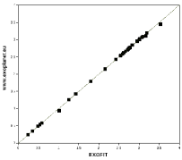
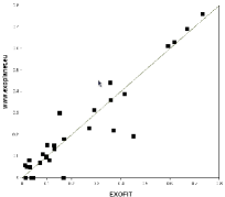
In this section we compare the published orbital periods and eccentricities of 30 extra-solar planets taken randomly from www.exoplanet.eu to that obtained by analyzing corresponding radial velocity data with EXOFIT . The results are summarized in Figure 2. It can be observed that the orbital periods extracted with EXOFIT matches closely with published ones. However, the eccentricities show apparent variation from the published values. In fact EXOFIT tends to obtain lower eccentricity solutions. This is clearly noticeable for planets with eccentricities greater that 0.5 (i.e. $\simeq$ 10% of the planet population). Median was used as the point estimator for marginal posterior distribution orbital parameters of exo-planets extracted with EXOFIT while comparing with the published results. This suggests that the orbital eccentricity is poorly constrained in many occasions because of the sparse sampling of the data points.

(a) Log(Period)

(b) Eccentricities

Figure 2.: Figure on the left plots $\log$(orbital period) of extra-solar planets, with results obtained by EXOFIT on the horizontal axis and published ones on the vertical axis. Figure on the right shows a comparison of orbital eccentricities with results obtained from EXOFIT on the horizontal axis and published ones on the vertical axis.

7. Summary and Future Work

We have introduced EXOFIT by reanalyzing the orbital solution of HD155358 by Cochran et al. (2007). EXOFIT provides a full Bayesian analysis of the problem and spits out the marginal posterior distribution of orbital parameters. We have also compared the orbital parameters obtained by EXOFIT to the published orbital solutions of 30 extra-solar planets taken randomly from www.exoplanet.eu, the objective being the reanalysis of the data using a single method and the estimation of corresponding orbital parameters and their uncertainties. The results show that while the orbital periods from EXOFIT agrees closely with the published ones, the eccentricities show significant variation from the published results. This fact indicates that orbital eccentricity is not accurately constrained and this degeneracy should be considered more carefully.

We plan to improve to the efficiency of EXOFIT by considering new parameterization for the problem as well as faster sampling techniques. Bayesian model selection will also be considered for the future versions of EXOFIT. We intend to extend our analysis to more planets and planetary data from transit photometry to provide a comprehensive Bayesian analysis of the statistical properties of orbital parameters of extra-solar planets.

Acknowledgments.

SB and OL would like to thank the organizers of the Molecules 2008 for giving the opportunity to attend the conference. SB would like the thank the organizing committee for the financial support provided. OL acknowledges the support of a Royal Society Wolfson Research Merit Award.

References

- Balan & Lahav (2008) Balan, S. T., & Lahav O., 2008, MNRAS, 394, 1936
- Cochran et al. (2007) Cochran, W. D., Endl, M., Wittenmyer, R. A., Bean, J. L., 2007, ApJ, 665, 1407
- Feroz & Hobson (2008) Feroz F., Hobson, M. P., 2008, MNRAS, 384, 449
- Ford (2005) Ford E. B, 2005, AJ, 129, 1706
- Gregory (2005a) Gregory, P. C. , 2005, ApJ, 631, 1198
- Jones et al. (2006) Jones, H. R. A., Butler, R. P., Tinney, C. G., Marcy, G. W., Carter, B. D, Penny, A. J., McCarthy, C., & Bailey J., 2006, MNRAS, 369, 249
- Lewis & Bridle (2002) Lewis, A., Bridle, S., 2002, Phys.Rev.D, 66, 103511
- Lomb (1973) Lomb, N. R. , 1976, Ap&SS, 39, 447
- Scargle (1982) Scargle, J. D. , 1982, ApJ, 263, 835