Sensor development and calibration for acoustic
neutrino detection in ice

Abstract

A promising approach to measure the expected low flux of cosmic neutrinos at the highest energies (E $>$ 1 EeV) is acoustic detection. There are different in-situ test installations worldwide in water and ice to measure the acoustic properties of the medium with regard to the feasibility of acoustic neutrino detection. The parameters of interest include attenuation length, sound speed profile, background noise level and transient backgrounds. The South Pole Acoustic Test Setup (SPATS) has been deployed in the upper 500 m of drill holes for the IceCube neutrino observatory at the geographic South Pole. In-situ calibration of sensors under the combined influence of low temperature, high ambient pressure, and ice-sensor acoustic coupling is difficult. We discuss laboratory calibrations in water and ice. Two new laboratory facilities, the Aachen Acoustic Laboratory (AAL) and the Wuppertal Water Tank Test Facility, have been set up. They offer large volumes of bubble free ice (3 m³) and water (11 m³) for the development, testing, and calibration of acoustic sensors. Furthermore, these facilities allow for verification of the thermoacoustic model of sound generation through energy deposition in the ice by a pulsed laser. Results from laboratory measurements to disentangle the effects of the different environmental influences and to test the thermoacoustic model are presented.

acoustic neutrino detection, thermoacoustic model, sensor calibration

1 Introduction

The detection and spectroscopy of extra-terrestrial ultra high energy neutrinos would allow us to gain new insights in the fields of astroparticle and particle physics. Apart from the possibility to study particle acceleration in cosmic sources, the measurement of the guaranteed flux of cosmogenic neutrinos [1] opens a new window to study cosmic source evolution and particle physics at unprecedented center of mass energies. However, the fluxes predicted for those neutrinos are very low [2], so detectors with large target masses are required for their detection. One possibility to instrument volumes of ice of the order of $100\,\mathrm{km}^{3}$ with a reasonable number of sensor channels is to detect the acoustic signal emitted from the particle cascade at a neutrino interaction vertex [3].

To study the properties of Antarctic ice relevant for acoustic neutrino detection the South Pole Acoustic Test Setup (SPATS) [4] has been frozen into the upper part of IceCube [5] boreholes. SPATS consists of four vertical strings reaching a depth of 500 m below the surface. The horizontal distances between strings cover the range from 125 m to 543 m. Each string is instrumented with seven acoustic sensors and seven transmitters. The ice parameters to be measured are the sound speed profile, the acoustic attenuation length, the background noise level, and transient noise events in the frequency range from 1 kHz to 100 kHz.

For the design of a large scale acoustic neutrino detector it is crucial to fully understand the in-situ response of the sensors as well as the thermoacoustic sound generation mechanism.

2 Sensor calibration

To study the acoustic properties of the Antarctic ice, like the absolute background noise level, and to deduce the arrival direction and energy of a neutrino in a future acoustic neutrino telescope it is essential to measure the sensitivity and directionality of the sensors used, i.e. the output voltage as function of the incident pressure, and its variation with the arrival direction of the incident acoustic wave relative to the sensor. These measurements can be carried out relatively easily in the laboratory in liquid water. The two calibration methods most commonly used are

• the comparison method, where an acoustic signal sent by a transmitter (with negligible angular variation) is simultaneously recorded at equal distance with a pre-calibrated receiver and the sensor to be calibrated. A comparison of the signal amplitudes in the two receivers allows for the derivation of the desired sensitivity from the sensitivity of the pre-calibrated sensor.

• the reciprocity method, which makes use of the electroacoustic reciprocity principle to determine the sensitivity of an acoustic receiver without having to use a pre-calibrated receiver (see e.g. [7]).

All SPATS sensors have been calibrated in $0\,^{\circ}$C water with the comparison method [8]. However, both calibration methods are not suitable for in-situ calibration of sensors in South Pole ice. There are no pre-calibrated sensors for ice available, and reciprocity calibration requires large setups which are not feasible for deployment in IceCube boreholes. Further, directionality studies require a change of relative positioning between emitter and receiver which is difficult to achieve in a frozen-in setup.

It is not clear how results obtained in the laboratory in liquid water can be transferred to an in-situ situation where the sensors are frozen into Antarctic ice. We are studying the influence of the following three environmental parameters on the sensitivity separately: low temperature, increased ambient pressure, and different acoustic coupling to the sensor. We will assume that sensitivity variations due to these factors obtained separately can be combined to a total sensitivity change for frozen in transmitters. This assumption can then be checked further using the two different sensor types deployed with the SPATS setup. Apart from the standard SPATS sensors with steel housing two HADES type sensors [9] have been deployed with the fourth SPATS string. These contain a piezoceramic sensor cast in resin and are believed to have different systematics.

2.1 Low temperatures

The ice temperature in the upper few hundred meters of South Pole ice is $-50\,^{\circ}$C [10]. It is not feasible to produce laboratory ice at this temperature in a large enough volume to carry out calibration studies. We study the dependence of the sensitivity on temperature in air. A signal sent by an emitter is recorded with a sensor at different temperatures. To prevent changes in the emissivity of the transmitter, the transmitter is kept at constant temperature outside the freezer, and only the sensor is cooled down. The recorded peak-to-peak amplitude is used as a measure of sensitivity. First results indicate a linear increase of sensitivity with decreasing temperature (cf. Fig. 1). The sensitivity of a SPATS sensor is increased by a factor of $1.5\pm 0.2$ when the temperature is lowered from $0\,^{\circ}$C to $-50\,^{\circ}$C (averaged over all three sensor channels).

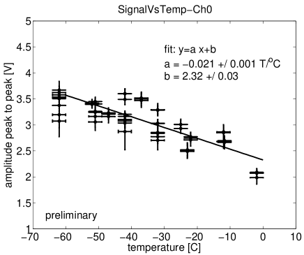
Figure 1: Measured peak-to-peak amplitude of one SPATS sensor channel in air at different temperatures and linear fit to the data.

2.2 Static pressure

Acoustic sensors in deep polar ice are exposed to increased ambient static pressure. During deployment this pressure is exerted by the water column in the borehole (max. 50 bar at 500 m depth). During re-freezing it increases since the hole freezes from the top, developing a confined water volume. The pressure is believed to decrease slowly as strain in the hole ice equilibrates to the bulk ice volume. The final static pressure on the sensor is unknown.

A $40.5$ cm inner diameter pressure vessel is available at Uppsala university that allows for studies of sensor sensitivity as function of ambient pressure. Static pressures between 0 and 800 bar can be reached. In this study the pressure is increased up to 100 bar. Acoustic emitters for calibration purposes can be placed inside the vessel or, free of pressure, outside of it. Cable feeds allow one to operate up to two sensors or transmitters inside the vessel. A sensor is placed in the center of the water filled vessel. The transmitter is coupled from the outside to the vessel. The recorded peak-to-peak amplitude is used as a measure of sensitivity while the pressure is increased. The sensor sensitivity is measured by transmitting single cycle gated sine wave signals with different central frequencies from 5 kHz to 100 kHz.

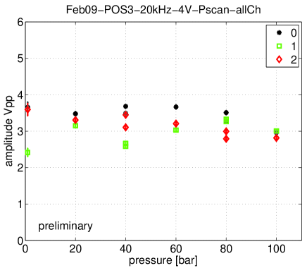
Figure 2: Measured peak-to-peak amplitude of a SPATS sensor excited by a transmitter coupled from the outside to the pressure vessel. All three channels of the sensor are shown.

Figure 2 shows the received signal amplitudes for the three sensor channels of a SPATS sensor as a function of ambient pressure. No systematic variation of the sensitivity with ambient pressure is observed. Combining all available data we conclude that the variation of sensitivity with static pressure is less than 30% for pressures below 100 bar.

2.3 Sensor-ice acoustic coupling

The acoustic coupling, i.e. the fractions of signal energy transmitted and reflected at the interface of medium and sensor, differs significantly between water and ice. It can be determined using the characteristic acoustic impedance of the medium and sensor, which is the product of density and sound velocity and is equivalent to the index of refraction in optics. Due to the different sound speeds the characteristic acoustic impedance of ice is about $2.5$ times higher than in water.

Its influence will be studied in the Aachen Acoustic Laboratory (Sec. 3), where it will be possible to carry out reciprocal sensor calibrations in both water and ice, and also to use laser induced thermoacoustic signals as a calibrated sound source.

3 New laboratory facilities

Two new laboratories have been made available to the IceCube Acoustic Neutrino Detection working group for signal generation studies and sensor development and calibration.

Wuppertal Water Tank Test Facility

For rapid prototyping of sensors and calibration studies in water, the Wuppertal Water Tank Test Facility offers a cylindrical water tank with a diameter of $2.5$ m and depth of $2.3$ m ($11\,\mathrm{m}^{3}$). The tank is built up from stacked concrete rings and has a walkable platform on top. It is equipped with a positioning system for sensors and transmitters and a 16-channel PC based DAQ system (National Instruments USB-6251 BNC).

The size of the water volume allows for the clean separation of emitted acoustic signals and their reflections from the walls and surface. This makes it possible to install triangular reciprocity calibration setups with side lengths of up to 1 m. Further, installations to measure the polar and azimuthal sensitivity of sensors are possible.

Aachen Acoustic Laboratory

The Aachen Acoustic Laboratory is dedicated to the study of thermoacoustic sound generation in ice. A schematic overview of the setup can be seen in Fig. 3. The main part is a commercial cooling container ($6\times 2.5\times 2.5\,\mathrm{m}^{3}$), which can reach temperatures down to $-25\,^{\circ}$C. An IceTop tank, an open cylindrical plastic tank with a diameter of 190 cm and a height of 100 cm [6], is located inside the container. The IceTop tank has a freeze control unit by means of which the production of bubble-free ice is possible. The freeze control unit mainly consists of a cylindrical semipermeable membrane at the bottom of the container, which is connected to a vacuum reservoir and a pressure regulation system. The membrane allows for degassing of the water. A total volume of $\approx 3\,\mathrm{m}^{3}$ of bubble-free ice can be produced. A full freezing cycle takes approximately sixty days with the freezing going from top to bottom.

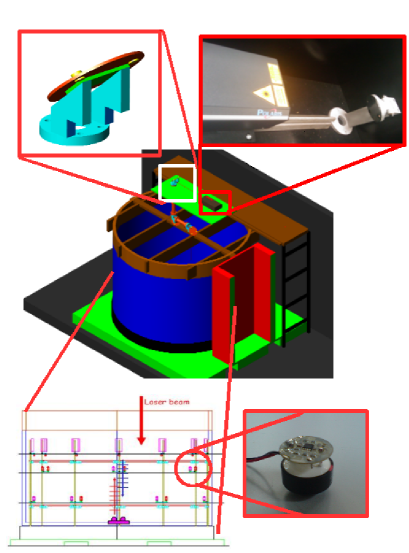
Figure 3: Overview of the AAL setup with zoom on the mirror holder (top), the sensor positioning system (bottom, left) and a sensor (bottom, right).

On top of the container, a Nd:YAG Laser is installed in a light-tight box with an interlock connected to the laser control unit. The laser has a pulse repetition rate of up to 20 Hz and a peak energy per pulse of 55 mJ at 1064 nm, 30 mJ at 532 nm, and 7 mJ at 355 nm wavelength. The laser beam is guided into the container and deposited in variable positions on the ice surface by a set of mirrors with coatings for the above mentioned frequencies. The optical feed-through consists of a tilted quartz window to avoid damage of the laser cavity by reflected laser light. For the detection of thermoacoustic signals, 18 sensors are mounted on a sensor positioning system. The positioning system has three levels, on each level 6 sensors are placed in a hexagonal geometry. Along with the sensors, 18 sound emitters are deployed for calibration and test purposes. The sensors will be calibrated reciprocally. The positioning system will also include a reciprocal calibration setup for HADES sensors and the ability to install a SPATS sensor for calibration purposes. In addition, two temperature sensors are deployed at each level. The acoustic sensors are pre-amplified low-cost piezo based ultrasound sensors, usually used for distance measurement. The sensors show a strong variation of signal strength with incident angle. This directionality has to be studied but is rather useful for the suppression of reflected signals. The sensors are read out continuously by a LabVIEW-based DAQ framework with a NI PCIe-6259M DAQ card. The framework includes a temperature and acoustic noise monitoring system.

4 Studies of thermoacoustic signal generation

A detailed understanding of thermoacoustic sound generation in ice is crucial for designing an acoustic extension to the IceCube detector. The dependence of the signal strength on the deposited energy as well as on the distance to the sensor is of great interest. Also the pulse shape and the frequency content have to be studied systematically with respect to various cascade parameters. The spatial distribution of the acoustic signal has to be investigated, i.e. the acoustic disk and its dependence on the spatial and temporal energy deposition distribution. In addition, the AAL setup will be able to study the thermoacoustic effect in a wide temperature range from $20\,^{\circ}$C to $-25\,^{\circ}$C and possible differences of the effect in ice and water.

In the Aachen Acoustic Laboratory, the thermoacoustic signal is generated by a Nd:YAG laser. A laser-induced thermoacoustic signal differs from a signal produced in a hadronic cascade. While a cascade’s energy deposition profile can be described by a Gaisser-Hillas function, the laser intensity drops of exponentially. Also the lateral profile of a cascade follows a NKG function, where, assuming a TEM₀₀ mode in the far field region, the typical laser-beam profile is Gaussian. Knowing this, a recalculation of the signal properties from a laser-induced pulse to a cascade-generated pulse is possible.

The frequency content of the signal is expected to vary with the beam diameter, while a too short penetration depth will result in an acoustic point source rather than a line source. The absorption coefficient of light in water or ice varies strongly with wavelength. The first wavelength of the laser (1064 nm) is absorbed after few centimeters, while the second harmonic (532 nm) has an absorption length of $\approx 60$ m. The third harmonic at 355 nm with an absorption length of $\approx 1$ m is expected to be the most suitable wavelength to emulate a hadronic cascade with a typical length of 10 m and a diameter of 10 cm. The diameter of the heated ice volume has to be controlled by optics inside the container that will widen the beam.

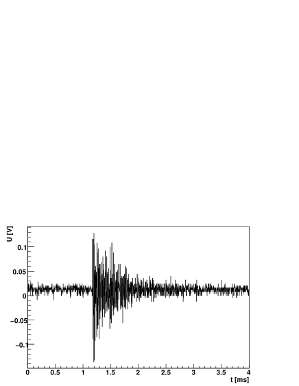
Figure 4: Thermoacoustic pulse in ice, generated with a laser at 1064 nm wavelength and a beam diameter of $\approx 1\,\mathrm{\mu m}$.

With an array of 18 sensors, the Aachen Acoustic Laboratory allows the study of the spatial distribution of the generated sound field, as well as the frequency content with varying beam parameters. The first thermoacoustic signal has been generated and detected in a test setup with preliminary sensor electronics in order to determine a reasonable gain for the pre-amplifier while avoiding saturation. A small volume of bubble-free ice has been produced, containing a sensor and an emitter. Laser pulses (wavelength 1064 nm, 55 mJ per pulse) have been shot at the ice block. A zoom on the first waveform is presented in Fig. 4. The distance between laser spot and sensor is approximately $15\,\mathrm{cm}$ and the sensor gain factor is 22. A Fourier transform of the pulse implies a pulse central frequency of $\approx 100\,\mathrm{kHz}$, which is expected for such a small beam diameter. In order to see the expected bipolar pulse, further studies have to be performed to determine the transfer function of the sensors.

5 Conclusions

Detailed understanding of the thermoacoustic sound generation mechanism and the response of acoustic sensors in Antarctic ice is necessary to design an acoustic extension for the IceCube neutrino telescope. While in-situ calibrations in deep South Pole ice are inherently difficult, different environmental influences can be studied separately in the laboratory. No change in sensor response with increasing ambient pressure was found; a linear increase in sensitivity with decreasing temperature was observed. Intense pulsed laser beams can be used to generate thermoacoustic signals in ice which can also be used as an in-ice calibration source.

References

- [1] V. S. Berezinsky and G. T. Zatsepin, Phys. Lett. B 28 (1969) 423.
- [2] R. Engel, D. Seckel and T. Stanev, Phys. Rev. D 64 (2001) 093010, arXiv:astro-ph/0101216.
- [3] G. A. Askaryan, At. Energ. 3 (1957) 152.
- [4] J. Vandenbroucke et al., Nucl. Instr. and Meth. A (2009), doi:10.1016/j.nima.2009.03.064, arXiv:0811.1087 [astro-ph].
- [5] http://icecube.wisc.edu/
- [6] T. K. Gaisser, in Proceedings of the 29th International Cosmic Ray Conference (ICRC 2005), arXiv:astro-ph/0509330.
- [7] R. J. Urick, Principles of underwater sound, 3rd ed., Peninsula Publishing (1983).
- [8] J.-H. Fischer, Diploma Thesis, Humboldt-Universität zu Berlin (2006).
- [9] B. Semburg et al., Nucl. Instr. and Meth. A (2009), doi:10.1016/j.nima.2009.03.069, arXiv:0811.1114 [astro-ph].
- [10] P. B. Price et al., Proc. Nat. Acad. Sci. U.S.A. 99 (2002) 7844.