Supersolidity in a Bose-Holstein model

Abstract

We derive an effective d-dimensional Hamiltonian for a system of hard-core-bosons coupled to optical phonons in a lattice. At non-half-fillings, a superfluid-supersolid transition occurs at intermediate boson-phonon couplings, while at strong-couplings the system phase separates. We demonstrate explicitly that the presence of next-nearest-neighbor hopping and nearest-neighbor repulsion leads to supersolidity. Thus we present a microscopic mechanism for the homogeneous coexistence of charge-density-wave and superfluid orders.

Introduction: Coexistence of charge-density-wave (CDW) and superconductivity is manifested in a variety of systems such as the perovskite type bismuthates (i.e., ${\rm BaBiO_{3}}$ doped with ${\rm K}$ or ${\rm Pb}$) blanton , quasi-two-dimensional layered dichalcogenides (e.g., ${\rm 2H-TaSe_{2}}$, ${\rm 2H-TaS_{2}}$, and ${\rm 2H-NbSe_{2}}$) withers , etc. What is special about the above systems is that they defy the usual expectation that the competing CDW and superconductivity orders occur mutually exclusively. CDW and superconductivity are examples of diagonal long range order (DLRO) and off-diagonal long range order (ODLRO) respectively. Here, DLRO breaks a continuous translational invariance into a discrete translational symmetry, whereas ODLRO breaks a global U(1) phase rotational invariance penrose .

Another interesting example of DLRO-ODLRO concurrence is a supersolid (SS). A SS state is characterized by the homogeneous coexistence of two seemingly mutually contradictory phases, namely, a crystalline solid and a superfluid (SF). Here all particles simultaneously participate in both types of long range order. It has been conjectured long ago that solid helium-4 may exhibit supersolidity due to Bose condensation of vacancies present Andreev ; leggett . Only recently, Chan and Kim (using a torsional oscillator) observed a decoupling of a small percentage of the helium solid from a container’s walls KimChan-Nature . They interpreted this as supersolidity. This discovery led to studies of bosonic models in different kinds of lattice structures Damle and with various types of particle interactions Sengupta . Phenomenologically, Ginzburg-Landau theory jinwu and a quantum solid based on Gross-Pitaevskii equation josserand have been used to study supersolidity.

In this paper, we address the above ongoing puzzles by studying the quantum phase transitions exhibited by hard-core-bosons (HCB) coupled to optical phonons. To this end, in contrast to the above treatments, we employ a microscopic approach involving a minimal Bose-Holstein (BH) lattice model. Examples of real systems describable by our BH model are as follows. In the bismuthate systems, the observed valence skipping of the bismuth ion is explained by invoking non-linear screening which is said to produce a large attractive interaction resulting in the formation of local pairs or HCB varma ; tvr . Such HCB couple to the cooperative breathing mode of the oxygen octahedra surrounding the Bismuth ion. In a helium-4 crystal, vacancies produce a local distortion and can be treated as HCB coupled to finite frequency phonons. Furthermore, the concentration of vacancies is very small leggett and hence direct interactions among these HCB is negligible. Lastly, for dichalcogenides such as ${\rm NbSe_{2}}$, where homogeneous coexistence of the two long range orders has been unambiguously established suderow , our results on the BH model should be quite relevant.

Figure 1: Quantum phase diagram at various particle numbers $N_{p}$, $t/\omega_{0}=1.0$ and (a) NNN hopping $J_{2}>0$ in our effective BH Hamiltonian [Eq. (5)] and (b) $J_{2}=0$ (xxz-model). Supersolidity occurs only in (a). The continuous lines in (a) and (b) are guides for the eye.

Starting with our BH model, we derive an effective d-dimensional Hamiltonian for HCB by using a transparent non-perturbative technique. The region of validity of our effective Hamiltonian is governed by the small parameter ratio of the adiabaticity $t/\omega_{0}$ and the boson-phonon (b-p) coupling $g$. The most interesting feature of this effective Hamiltonian is that it contains an additional next-nearest-neighbor (NNN) hopping compared to the Heisenberg xxz-model involving only nearest-neighbor (NN) hopping and NN repulsion micnas ; ranninger2 . We employed a modified Lanczos algorithm gagli (on lattices of sizes $4\times 4$, $\sqrt{18}\times\sqrt{18}$, $\sqrt{20}\times\sqrt{20}$, and $4\times 6$) and found that (except for the extreme anti-adiabatic limit) the BH model shows supersolidity at intermediate b-p coupling strengths whereas the xxz-model produces only a phase separated (PS) state. Here we present the calculations for only a $4\times 4$ lattice (see Fig. 1). Our main results are depicted in Fig. 1 (a), where supersolidity manifested by local pairs (as HCB) implies homogeneous coexistence of CDW and superconductivity.

Effective Bose-Holstein Hamiltonian: We start with a system of spinless HCB coupled with optical phonons on a square lattice. This system is described by a BH Hamiltonian ranninger1

$$H=-t\sum_{j,\delta}b^{\dagger}_{j}b_{j+\delta}+\omega_{0}\sum_{j}a^{\dagger}_{j}a_{j}+g\omega_{0}\sum_{j}n_{j}(a_{j}+a^{\dagger}_{j}),$$ (1)

where $\delta$ corresponds to nearest-neighbors, $\omega_{0}$ is the optical phonon frequency, $b_{j}$ ($a_{j}$) is the destruction operator for HCB (phonons), and $n_{j}\equiv b^{\dagger}_{j}b_{j}$. Then we perform the Lang-Firsov (LF) transformation lang ; sdadys on this Hamiltonian and this produces displaced simple harmonic oscillators and dresses the hopping particles with phonons. Under the LF transformation given by $e^{S}He^{-S}=H_{0}+H^{\prime}$ with $S=-g\sum_{i}n_{i}(a_{i}-a^{\dagger}_{i})$, $b_{j}$ and $a_{j}$ transform like fermions and phonons in the Holstein model. This is due to the unique (anti-) commutation properties of HCB given by

$$[b_{i},b_{j}] = [b_{i},b^{\dagger}_{j}]=0,\textrm{ for }i\neq j,$$

$$\{b_{i},b^{\dagger}_{i}\} = 1.$$ (2)

Next, we take the unperturbed Hamiltonian $H_{0}$ to be sdadys

$$H_{0}=-J_{1}\sum_{j,\delta}b^{\dagger}_{j}b_{j+\delta}+\omega_{0}\sum_{j}a^{\dagger}_{j}a_{j}-g^{2}\omega_{0}\sum_{j}n_{j},$$ (3)

and the perturbation $H^{\prime}$ to be

$$H^{\prime}=-J_{1}\sum_{j,\delta}b^{\dagger}_{j}b_{j+\delta}\{\mathcal{S}^{{j}^{\dagger}}_{+}\mathcal{S}^{j}_{-}-1\},$$ (4)

where $\mathcal{S}^{j}_{\pm}=\textrm{exp}[\pm g(a_{j}-a_{j+\delta})],J_{1}=t\textrm{exp}(-g^{2})$, and $g^{2}\omega_{0}$ is the polaronic binding energy. We then follow the same steps as in Ref. [sdadys, ] to get the following effective Hamiltonian in d-dimensions for our BH model

$$\!\!\!\!H_{e}\!\! = \!\!-g^{2}\omega_{0}\sum_{j}n_{j}-J_{1}\sum_{j,\delta}b^{\dagger}_{j}b_{j+\delta}$$ (5)

$$\!\!\!\!\!\!-J_{2}\sum_{j,\delta,\delta^{\prime}\neq\delta}b^{\dagger}_{j+\delta^{\prime}}b_{j+\delta}-0.5J_{z}\sum_{j,\delta}n_{j}(1-n_{j+\delta}),$$

where $J_{z}\equiv(J_{1}^{2}/\omega_{0})[4f_{1}(g)+2f_{2}(g)]$ and $J_{2}\equiv(J_{1}^{2}/\omega_{0})f_{1}(g)$ with $f_{1}(g)\equiv\sum^{\infty}_{n=1}g^{2n}/(n!n)$ and $f_{2}(g)\equiv\sum^{\infty}_{n=1}\sum^{\infty}_{m=1}g^{2(n+m)}/[n!m!(n+m)].$ Here we would like to point out that, as shown in Ref. sudhakar1, , the small parameter for our perturbation theory is $t/(g\omega_{0})$.

Long range orders: Diagonal long range order (DLRO) can be characterized by the structure factor defined in terms of the particle density operators as follows:

$$S(\mathbf{q})=\frac{1}{N}\sum_{i,j}e^{\mathbf{q}\cdot(\mathbf{R}_{i}-\mathbf{R}_{j})}(\left\langle n_{i}n_{j}\right\rangle-\left\langle n_{i}\right\rangle\left\langle n_{j}\right\rangle).$$ (6)

Off-diagonal long range order (ODLRO) in a Bose-Einstein condensate (BEC), as introduced by Penrose and Onsager penrose , is characterized by the order parameter $\left<b_{0}\right>=\sqrt{\left<n_{0}\right>}e^{i\theta}$ where $n_{0}$ is the occupation number for the $\mathbf{k}=0$ momentum state or the BEC. It is useful to define the general one-particle density matrix

$$\tilde{\rho}(i,j)=\left<b^{\dagger}_{i}b_{j}\right>=\frac{1}{N}\sum_{\mathbf{k},\mathbf{q}}e^{(\mathbf{k}\cdot\mathbf{R}_{i}-\mathbf{q}\cdot\mathbf{R}_{j})}\left<b^{\dagger}_{\mathbf{k}}b_{\mathbf{q}}\right>,$$ (7)

where $\left<\right>$ denotes ensemble average. Eq. (7) gives the BEC fraction as

$$n_{b}=\frac{\left<n_{0}\right>}{N_{p}}=\sum_{i,j}\frac{\tilde{\rho}(i,j)}{NN_{p}}.$$ (8)

In general, to find $n_{b}$, one constructs the generalized one-particle density matrix $\tilde{\rho}$ and then diagonalizes it to find out the largest eigenvalue. To characterize a SF, an important quantity is the SF fraction $n_{s}$ which is calculated as follows. Spatial variation in the phase of the SF order parameter will increase the free energy of the system. We use a linear phase variation $\theta(x)=\theta_{0}(x/L)$ with $\theta_{0}$ being a small angle and $L$ the linear dimension in x-direction. This is done by imposing twisted boundary conditions (TBC) on the many-particle wave function. At $T=0$ K, we can write the change in energy to be

$$E[\theta_{0}]-E[0]=\frac{1}{2}mN_{p}n_{s}\left|\frac{\hbar}{m}\vec{\nabla}\theta(x)\right|^{2}.$$ (9)

Then the SF fraction is given by fisher ; roth

$$n_{s}=\left(\frac{N}{N_{p}t_{eff}}\right)\frac{E[\theta_{0}]-E[0]}{\theta_{0}^{2}},$$ (10)

where $t_{eff}=\hbar^{2}/2m$. For our Hamiltonian in Eq. (5), we find $t_{eff}=J_{1}+8J_{2}$. The phase variation (taken to be the same for BEC and SF order parameters) is introduced in our calculations by modifying the hopping terms with $b_{j}\rightarrow b_{j}\exp[i\hat{\mathbf{x}}\cdot\mathbf{R}_{j}\theta_{0}/L]$ which is gauge-equivalent to TBC.

Results and discussion: We employ the mean field analysis (MFA) of Robaszkiewicz et al. micnas to study the phase transitions dictated by the effective Hamiltonian of Eq. (5). We obtain the following expression for the SF-PS (SF-CDW) phase boundary at non-half-filling (half-filling):

$$\frac{J_{z}}{2J_{1}}-\frac{3J_{2}}{J_{1}}=\frac{1+\left(2n-1\right)^{2}}{1-\left(2n-1\right)^{2}}.$$ (11)

Eq.(11) leads to the same phase diagram as that (for the xxz-model) in Ref. micnas, but with $J^{eff}_{z}=J_{z}/2-3J_{2}$ as the y-coordinate instead of $J^{eff}_{z}=J_{z}/2$. Thus, within mean field, NNN hopping does not change the qualitative features of the phase diagram; it only increases the critical value of ${J_{z}}/{J_{1}}$ at which the transition from SF state to PS or CDW state occurs. However, as demonstrated by the numerics below at non-half-fillings, MFA fails to capture the supersolid phase.

We studied the stability of the phases by examining the nature of the free energy versus $N_{p}$ curves at different b-p couplings $g$ (see Figs. 2 and 3) and by using an analysis equivalent to the Maxwell construction. For the system at a given $N_{p}$, $g$, and $t/\omega_{0}$, if the free energy point $P$ lies above the straight line joining the nearest two stable points $Q$ and $R$ (lying on either side of $P$) on the same free energy curve, then the system at $P$ breaks up into two phases corresponding to points $Q$ and $R$.

For the range of parameters that we considered (i.e., $0.1\leq t/\omega_{0}\leq 1$ and $g>1$), the small parameter $t/(g\omega_{0})<1$. The behavior of the system for $t/\omega_{0}=0.1$ is the same for both $J_{2}=0$ and $0\neq J_{2}/J_{1}$ [= $(J_{1}/\omega_{0})f_{1}(g)$] because $J_{2}/J_{1}$ is negligible in the latter case. Furthermore, for $J_{2}=0$, the behavior of the system as a function of $g$ is qualitatively the same for all values of $t/\omega_{0}$ as there is only one dimensionless parameter $J_{z}/J_{1}$ involved in Eq. (5).

Figure 2: Free energy at different fillings and different values of $g$ for (a) $J_{1}>0$, $J_{2}\neq 0$, and $t/\omega_{0}=0.1$; and (b) $J_{1}=0$, $J_{2}\neq 0$, and $t/\omega_{0}=1.0$.

Figure 3: Plot of free energy for different number of particles and various values of $g$ when $J_{1}\neq 0$, $J_{2}\neq 0$, and $t/\omega_{0}=1.0$.

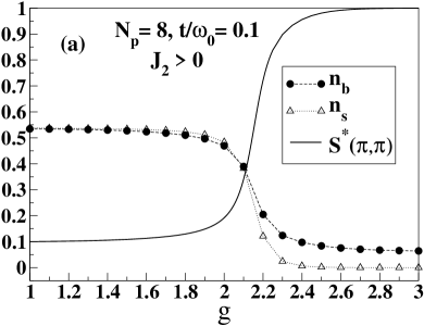
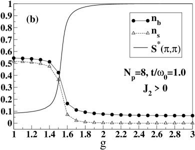
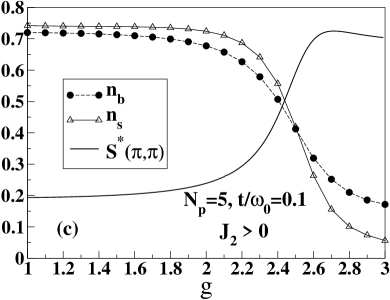
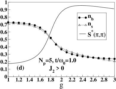
Figure 4: Comparative plots of $S^{*}(\pi,\pi)$, $n_{b}$, and $n_{s}$ when $J_{1}\neq 0$, $J_{2}\neq 0$, and (a) $t/\omega_{0}=0.1$, $N_{p}=8$; (b) $t/\omega_{0}=1.0$, $N_{p}=8$; (c) $t/\omega_{0}=0.1$, $N_{p}=5$; and (d) $t/\omega_{0}=1.0$, $N_{p}=5$.

We will now analyze together, in one plot, the quantities $n_{b}$, $n_{s}$, and the normalized structure factor $S^{*}(\pi,\pi)=S(\pi,\pi)/S^{max}(\pi,\pi)$ where $S^{max}(\pi,\pi)$ corresponds to all particles occupying only one sub-lattice. At half-filling, we first observe that the system is either a pure CDW or a pure SF. For a half-filled system (i.e., $N_{p}=8$) at $J_{2}\neq 0$ and $t/\omega_{0}=0.1$ ($t/\omega_{0}=1.0$), we can see from Fig. 4 (a) [Fig. 4 (b)] that the system undergoes a sharp (first order) transition to an insulating CDW state at $g_{c}\approx 2.15$ ($g_{c}\approx 1.55$). At $g=g_{c}$, while there is a sharp rise in $S^{*}(\pi,\pi)$, there is also a concomitant sharp drop in both the condensation fraction $n_{b}$ and the SF fraction $n_{s}$. Furthermore, while $n_{s}$ actually goes to zero, $n_{b}$ remains finite [as follows from Eq. (8)] at a value $1/N=1/16$ which is an artifact of the finiteness of the system. Larger values of $t/\omega_{0}$ for a half-filled system leads to lower values of $g_{c}$. This is in accordance with the MFA phase boundary Eq. (11) and the fact that $(J_{z}/J_{1})\times(\omega_{0}/t)$ [$(J_{2}/J_{1})\times(\omega_{0}/t)$] is monotonically increasing (decreasing) function of $g$ for $g>1$.

Away from half-filling, the system shows markedly different behavior compared to the half-filled situation. For $N_{p}\leq 4$ in the $4\times 4$ lattice considered here, without actually presenting the details of the calculations, we first note that there is no evidence of a phase transition (for both $J_{2}=0$ and $J_{2}\neq 0$).

In Fig. 4 (c) drawn for $N_{p}=5$, although $S^{*}(\pi,\pi)$ displays a CDW transition at a critical value $g_{c}=2.45$, $n_{s}$ does not go to zero even at large values of $g$ considered. Furthermore, we see clearly from Fig. 2 (a) that, above this critical value of $g$, the curvature of the free energy curves suggests that the system at $N_{p}=5$ is an inhomogeneous mixture of CDW-state and SF-state. Thus away from half-filling, at small values of the adiabaticity $t/\omega_{0}$, our HCB-system undergoes a transition from a SF-state to a PS-state at a critical b-p coupling strength [similar to the xxz-model in Fig. 1 (b)].

However for $t/\omega_{0}$ not too small, when NNN hopping is present, the system shows a strikingly new behavior for a certain region of the $g$-parameter space. Let us consider the system at $N_{p}=5$, $t/\omega_{0}=1.0$, $J_{1}\neq 0$, and $J_{2}\neq 0$. Fig. 4 (d) shows that, above $g\approx 1.85$, the system enters a CDW state (as can be seen from the structure factor); however, it continues to have a SF character as reflected by the finite value of $n_{s}$. Furthermore, Fig. 3 reveals that the curve is concave, i.e., the system is PS, only above $g=2.0$. This simultaneous presence of CDW and SF states, without any inhomogeneity (for $1.85<g<2.1$), implies that the system is a supersolid. Similarly, for $6$ and $7$ particles as well, we find that the system undergoes transition from a SF-state to a SS-state and then to a PS-state. This behavior is displayed in Fig. 1 (a).

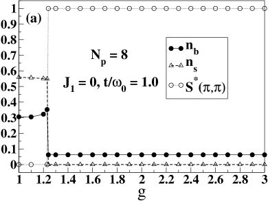
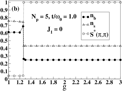
Figure 5: Comparison of $S^{*}(\pi,\pi)$, $n_{b}$, and $n_{s}$ when $t/\omega_{0}=1.0$, $J_{2}\neq 0$ but $J_{1}=0$ and for (a) $N_{p}=8$; and (b) $N_{p}=5$.

Finally, we shall present the interesting case of $J_{1}=0$ and $J_{2}\neq 0$ as a means of understanding the SS phase in the phase diagram of Fig. 1 (a). The physical scenario, when $J_{1}$ can be negligibly small compared to $J_{2}$, has been addressed in Ref. [sudhakar1, ] for cooperative electron-phonon interaction in an one-dimensional system. When $J_{1}=0$, for large values of nearest-neighbor repulsion, it is quite natural that all the particles will occupy a single sub-lattice. However, the dramatic jump (at a critical value of $g$), from an equal occupation of both sub-lattices to a single sub-lattice occupation, is quite unexpected (see Fig. 5). For a half-filled system, above a critical point, all the particles get localized which results in an insulating state. This can be seen from Fig. 5 (a). One can see that (at $g\approx 1.23$) the structure factor dramatically jumps to its maximum value, while $n_{s}$ drops to zero and $n_{b}$ takes the limiting value of $1/16$ for reasons discussed earlier. This shows that above $g\approx 1.23$, the system is in an insulating state with one sub-lattice being completely full. However, away from half-filling, the system conducts perfectly while occupying a single sub-lattice because of the presence of holes in the sub-lattice. For instance, from Fig. 5 (b) drawn for $N_{p}=5$, we see that the structure factor jumps to its maximum value at $g\approx 1.26$, whereas $n_{s}$ drops to a finite value which remains constant above $g=1.26$. We see from Fig. 2 (b), based on the curvature of the free energy curves, that the 5-particle system does not phase separate both above and below the CDW transition. In fact, this single-phase-stability is true for any filling. This means that the system, at any non-half filling and at $J_{1}=0$, exhibits supersolidity above a critical value of $g$!

Conclusions: We demonstrated that our BH model displays supersolidity in two-dimensions (2D). Our effective Hamiltonian of Eq. (5) should be realizable in a 2D optical lattice. Furthermore, our BH model too can be mimicked by designing HCB to move as extra particles in a 2D array of trapped molecules with HCB coupled to the breathing mode of the trapped molecules zoller . In three-dimensions, supersolidity is more achievable (i) in general, due to an increase in the ratio of NNN and NN coordination-numbers; and (ii) in particular for bismuthates, because cooperative breathing mode enhances the ratio of NNN and NN hoppings.

S. Datta thanks Arnab Das for very useful discussions on implementation of Lanczos algorithm. S. Yarlagadda thanks K. Sengupta, S. Sinha, A. V. Balatsky, R. J. Cava, I. Mazin, and M. Randeria for valuable discussions. This research was supported in part by the National Science Foundation under Grant No. PHY05-51164 at KITP.

References

- (1) S. H. Blanton et al., Phys. Rev. B 47, 996 (1993).
- (2) For a review, see R. L. Withers and J. A. Wilson, J. Phys. C 19, 4809 (1986).
- (3) O. Penrose and L. Onsager, Phys. Rev. 104, 576 (1956).
- (4) A. F. Andreev and I. M. Lifshitz, Sov. Phys. JETP 29, 1107 (1969); G. V. Chester, Phys. Rev. A 2, 256 (1970).
- (5) A. J. Leggett, Phys. Rev. Lett. 25, 1543 (1970).
- (6) E. Kim and M. H. W. Chan, Nature 427, 225 (2004).
- (7) D. Heidarian and K. Damle, Phys. Rev. Lett. 95, 127206 (2005); R. G. Melko et al., ibid. 95, 127207 (2005); S. Wessel and M. Troyer, ibid. 95 127205 (2005).
- (8) P. Sengupta et al., Phys. Rev. Lett. 94, 207202 (2005).
- (9) Jinwu Ye, Phys. Rev. Lett. 97, 125302 (2006).
- (10) C. Josserand, Y. Pomeau, and S. Rica, Phys. Rev. Lett. 98, 195301 (2007).
- (11) C. M. Varma, Phys. Rev. Lett. 61, 2713 (1988).
- (12) A. Taraphder, H. R. Krishnamurthy, Rahul Pandit, and T. V. Ramakrishnan, Phys. Rev. B 52, 1368 (1995).
- (13) H. Suderow et al., Phys. Rev. Lett. 95, 117006 (2005).
- (14) S. Robaszkiewicz, R. Micnas, and K. A. Chao, Phys. Rev. B 23, 1447 (1981).
- (15) A. S. Alexandrov and J. Ranninger, Phys. Rev. B 23, 1796 (1981); A. S. Alexandrov, J. Ranninger, and S. Robaszkiewicz , Phys. Rev. B 33, 4526 (1986).
- (16) E. R. Gagliano et al., Phys. Rev. B 34, 1677 (1986).
- (17) G. Jackeli and J. Ranninger, Phys. Rev. B 63, 184512 (2001).
- (18) S. Datta, A. Das, and S. Yarlagadda, Phys. Rev. B 71, 235118 (2005).
- (19) I.G. Lang and Yu.A. Firsov, Zh. Eksp. Teor. Fiz. 43, 1843 (1962) [Sov. Phys. JETP 16, 1301 (1962)].
- (20) S. Yarlagadda, arXiv:0712.0366v2.
- (21) M. E. Fisher, M. N. Barber, and D. Jasnow, Phys. Rev. A 8, 1111 (1973).
- (22) R. Roth and K. Burnett, Phys. Rev. A 68, 023604 (2003).
- (23) For a similar system, see G.Pupillo et al., Phy. Rev. Lett 100, 050402 (2008).