Scl, sails and surgery

Abstract.

We establish a close connection between stable commutator length in free groups and the geometry of sails (roughly, the boundary of the convex hull of the set of integer lattice points) in integral polyhedral cones. This connection allows us to show that the scl norm is piecewise rational linear in free products of Abelian groups, and that it can be computed via integer programming. Furthermore, we show that the scl spectrum of nonabelian free groups contains elements congruent to every rational number modulo $\mathbb{Z}$, and contains well-ordered sequences of values with ordinal type $\omega^{\omega}$. Finally, we study families of elements $w(p)$ in free groups obtained by surgery on a fixed element $w$ in a free product of Abelian groups of higher rank, and show that $\textnormal{scl}(w(p))\to\textnormal{scl}(w)$ as $p\to\infty$.

1. Introduction

Bounded cohomology, introduced by Gromov in [14], proposes to quantify homology theory, replacing groups and homomorphisms with Banach spaces and bounded linear maps. In principle, the information contained in the bounded cohomology of a space is incredibly rich and powerful; in practice, except in (virtually) trivial cases, this information has proved impossible to compute. Burger-Monod [6] wrote the following in 2000:

Although the theory of bounded cohomology has recently found many applications in various fields … for discrete groups it remains scarcely accessible to computation. As a matter of fact, almost all known results assert either a complete vanishing or yield intractable infinite dimensional spaces.

Perhaps the best known exceptions are Gromov’s theorem [14] that the norm of the fundamental class of a hyperbolic manifold is proportional to its volume, and Gabai’s theorem [12] that the Gromov norm on $H_{2}$ of an atoroidal $3$-manifold is equal to the Thurston norm. Even these results only describe a finite dimensional sliver of the (typically) uncountable dimensional bounded cohomology groups of the spaces in question.

The case of $2$-dimensional bounded cohomology is especially interesting, since it concerns extremal maps of surfaces into spaces. In virtually every category it is important to be able to construct and classify surfaces of least complexity mapping to a given target; we mention only minimal surface theory and Gromov-Witten theory as prominent examples. In the topological category one wants to minimize the genus of a surface mapping to some space subject to further constraints (e.g. that the image represent a given homology class, that it be $\pi_{1}$-injective, that it be a Heegaard surface, etc.) For many applications (e.g. inductive arguments) it is crucial to relativize this problem: given a space $X$ and a (homologically trivial) loop $\gamma$ in $X$, one wants to find a surface of least complexity (again, perhaps subject to further constraints) mapping to $X$ in such a way as to fill $\gamma$ (i.e. $\gamma$ becomes the boundary of the surface). The problem of computing the genus of a knot (in a $3$-manifold) is of this kind. On the algebraic side, the relevant (bounded) homological tool to describe complexity in this context is stable commutator length. In a group $G$, the commutator length $\textnormal{cl}(g)$ of an element $g$ is the least number of commutators whose product is $g$, and the stable commutator length $\textnormal{scl}(g)$ is the limit $\textnormal{scl}(g)=\lim_{n\to\infty}\textnormal{cl}(g^{n})/n$. Here, until very recently, the landscape was even more barren: there were virtually no examples of groups or spaces in which stable commutator length could be calculated exactly where it did not vanish identically ([20] is an interesting exception).

The paper [7] successfully showed how to compute stable commutator length in a highly nontrivial example: that of free groups. The result is very interesting: stable commutator length turns out to be rational, and for every rational $1$-boundary, there is a (possibly not unique) best surface which fills it rationally, in a precise sense. The case of a free group is important for several reasons:

1. Computing scl in free groups gives universal estimates for scl in arbitrary groups

2. The category of surfaces and maps between them up to homotopy is a fundamental mathematical object; studying scl in free and surface groups gives a powerful new framework in which to explore this category

3. Free groups are the simplest examples of hyperbolic groups, and are a model for certain other families of groups (mapping class groups, $\textnormal{Out}(F_{n})$, groups of symplectomorphisms) that exhibit hyperbolic behavior

The paper [7] gives an algorithm to compute scl on elements in a free group. Refinements (see [8], Ch. 4) show how to modify this algorithm to make it polynomial time in word length. Hence it has become possible to calculate (by computer) the value of scl for words of length $\sim 60$ in a free group on two generators. The utility of this is to make it possible to perform experiments, which reveal the existence of hitherto unsuspected phenomena in the scl spectrum of a free group. These phenomena suggest many new directions for research, some of which are pursued in this paper.

Figure 1 is a histogram of values of scl between $1$ and $\frac{5}{4}$ on alternating words of length $28$ in the (commutator subgroup of the) free group on two generators. Here a word is alternating if the letters alternate between one of $a^{\pm 1}$ and one of $b^{\pm 1}$.

2pt $1$ at 10 -20 $\frac{15}{14}$ at 152.857142 -20 $\frac{13}{12}$ at 176.666667 -20 $\frac{11}{10}$ at 210 -20 $\frac{9}{8}$ at 260 -20 $\frac{8}{7}$ at 295.714286 -20 $\frac{7}{6}$ at 343.333333 -20 $\frac{17}{14}$ at 438.571428 -20 $\frac{19}{16}$ at 385 -20 $\frac{6}{5}$ at 410 -20 $\frac{5}{4}$ at 510 -20

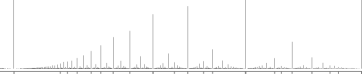
Figure 1. Histogram of values of scl on alternating words of length $28$ in $F_{2}$. Heights of the bars at $1$ and $\frac{5}{4}$ have been truncated to fit in the Figure.

The most salient feature of this histogram is its self-similarity. Such self-similarity is indicative of a power law roughly of the form $\textnormal{freq}(p/2q)\sim q^{-\delta}$ for some $\delta$ which in this case is about $2.1$ (although there is some interesting irregularity even in this figure, e.g. the curiously “high” spike at $\frac{29}{28}$ and “low” spike at $\frac{39}{41}$).

Unfortunately, the algorithm developed in [8] is not adequate to explain the structure evident in Figure 1. One reason is that this algorithm reduces the calculation of scl on a particular element of $F_{2}$ to a linear programming problem, the particulars of which depend in quite a dramatic way on the word in question. Moreover, though the algorithm is polynomial time in word length, it is not polynomial time in “log exponent word length”, i.e. the notation which abbreviates a word like $aaaaaaaba^{-1}a^{-1}a^{-1}baab^{-1}b^{-1}$ to $a^{7}ba^{-3}ba^{2}b^{-2}$. This is especially vexing in view of the fact that experiments suggest a rich structure for the values of scl on families of words which differ only in the values of their exponents. This is best illustrated with an example.

Example 1.1.

In $F_{2}$ with generators $a,b$, experiments suggest a formula

$$\textnormal{scl}(aba^{-1}b^{-1}ab^{-n}a^{-1}b^{n})=1-\frac{1}{2n-2}$$

valid for $n\geq 2$.

There are two interesting aspects of this example: the fact that the values of scl (apparently) converge to a (rational) limit, and the nature of the error term (which is a harmonic series). One of the goals of this paper is to develop a different approach to computing scl in free groups (and some other classes of groups) which makes it possible to rigorously verify and to explain the phenomena exhibited in Example 1.1 and more generally.

1.1. Sails

One surprising thing to come out of this paper is the discovery of a close connection between stable commutator length in free groups, and the geometry of sails in integral polyhedral cones. Given an integral polyhedral cone $V$ the sail of $V$ is the convex hull of $\mathcal{D}+V$, where $\mathcal{D}$ is the set of integral lattice points in certain open faces of $V$ (this is a generalization of the usual definition of a sail, in which one takes for $\mathcal{D}$ the set of all integer lattice points in $V$ except for the vertex of the cone). Sails were introduced by Klein, in his attempt to generalize to higher dimensions the theory of continued fractions. Given a cone $V$, define the Klein function $\kappa$ to be the function on $V$, linear on rays, that is equal to $1$ exactly on the sail. It turns out that calculating scl on chains in free products of Abelian groups reduces to the problem of maximizing a function $-\chi/2$ on a certain rational polyhedron (obtained by intersecting the product of two integral polyhedral cones with a rational affine subspace). The function $-\chi/2$ is the sum of two terms, one linear, and one which is (the restriction of) a sum of Klein functions associated to the two polyhedral cones.

This connection will be discussed further in a future paper, especially as it relates to the statistical features evident e.g. in Figure 1.

1.2. Stallings

If $A$ and $B$ are groups, one can build a $K(A*B,1)$ by wedging a $K(A,1)$ and a $K(B,1)$ along a basepoint. Given a surface $S$ and a map $f:S\to K(A*B,1)$ one can try to simplify $S$ and $f$ in two complementary ways: either by simplifying the part of $S$ that maps to the two factors, or by simplifying the part that maps to the basepoint. In a precise sense, the first strategy was pursued in [7] whereas the second strategy is pursued in this paper.

An interesting precursor of this latter approach is John Stallings’ last paper [18], which uses topological methods to factorize products of commutators in a free product of groups into terms which are localized in the factors. It is a pleasure to acknowledge my own great intellectual debt to John, and it seems especially serendipitous to discover, in relatively unheralded work he did in the later part of his life, some beautiful new ideas which continue to inform and inspire.

1.3. Main results

We now briefly describe the contents of the paper. In § 2 we give definitions, standardize notation, and recall some fundamental facts from the theory of stable commutator length, especially the geometric definition in terms of maps of surfaces to spaces.

In § 3 we describe a method to compute stable commutator length in free products of Abelian groups. We show that the computation can be reduced to a kind of integer programming problem, exhibiting a natural connection between the stable commutator length in free groups, and the geometry of sails in integral polyhedral cones (this is explained in more detail in the sequel). As a consequence, we derive our first main theorem:

Rationality Theorem.

Let $G=*_{i}A_{i}$ be a free product of finitely many finitely generated free Abelian groups. Then scl is a piecewise rational linear function on $B_{1}^{H}(G)$. Moreover, there is an algorithm to compute scl in any finite dimensional rational subspace.

In § 4 we exploit the relationship between scl and sails developed in the previous section, and use this to compute scl on an explicit multi-parameter infinite family of chains in $B_{1}^{H}(F_{2})$. This calculation enables us to rigorously verify the existence of certain phenomena in the scl spectrum that were suggested by experiments. Explicitly, this calculation allows us to prove:

Denominator Theorem.

The image of a nonabelian free group of rank at least $4$ under scl in $\mathbb{R}/\mathbb{Z}$ is precisely $\mathbb{Q}/\mathbb{Z}$.

and

Limit Theorem.

For each $n$, the image of the free group $F_{n}$ under scl contains a well-ordered sequence of values with ordinal type $\omega^{\lfloor n/4\rfloor}$. The image of $F_{\infty}$ under scl contains a well-ordered sequence of values with ordinal type $\omega^{\omega}$.

Finally, we obtain a result that explains the existence of many limit points in the scl spectrum of free groups. Let $A*B$ and $A^{\prime}*B$ be free products of free Abelian groups. A line of surgeries is a family of surjective homomorphisms $\rho_{p}:A*B\to A^{\prime}*B$ determined by a linear family of surjective homomorphisms on the factors.

Surgery Theorem.

Fix $w\in B_{1}^{H}(A*B)$ and let $\rho_{p}:A*B\to A^{\prime}*B$ be a line of surgeries, constant on the second factor, and surjective on the first factor with $\textnormal{rank}(A^{\prime})=\textnormal{rank}(A)-1$. Define $w(p)=\rho_{p}(w)$. Then $\lim_{p\to\infty}\textnormal{scl}(w(p))=\textnormal{scl}(w)$.

2. Background

This section contains definitions and facts which will be used in the sequel. A basic reference is [8].

2.1. Definitions

The following definition is standard; see [3].

Definition 2.1.

Let $G$ be a group, and $g\in[G,G]$. The commutator length of $g$, denoted $\textnormal{cl}(g)$, is the smallest number of commutators in $G$ whose product is $g$. The stable commutator length of $g$, denoted $\textnormal{scl}(g)$, is the limit

$$\textnormal{scl}(g)=\lim_{n\to\infty}\frac{\textnormal{cl}(g^{n})}{n}$$

Commutator length and stable commutator length can be extended to finite linear sums of groups elements as follows:

Definition 2.2.

Let $G$ be a group, and $g_{1},g_{2},\cdots,g_{m}$ elements of $G$ whose product is in $[G,G]$. Define

$$\textnormal{cl}(g_{1}+\cdots+g_{m})=\inf_{h_{i}\in G}\textnormal{cl}(g_{1}h_{1}g_{2}h_{1}^{-1}\cdots h_{m-1}g_{m}h_{m-1}^{-1})$$

and

$$\textnormal{scl}(g_{1}+\cdots+g_{m})=\lim_{n\to\infty}\frac{\textnormal{cl}(g_{1}^{n}+\cdots+g_{m}^{n})}{n}$$

Remark 2.3.

Note that scl will be finite if and only if the product of the $g_{i}$ is trivial in $H_{1}(G;\mathbb{Q})$.

The function scl may be interpreted geometrically as follows.

Definition 2.4.

Let $S$ be a compact surface with components $S_{i}$. Define

$$\chi^{-}(S)=\sum_{i}\min(0,\chi(S_{i}))$$

where $\chi$ denotes Euler characteristic.

In words, $\chi^{-}(S)$ is the sum of the Euler characteristics over all components of $S$ for which $\chi$ is non-positive.

Definition 2.5.

Let $g_{1},g_{2}\cdots g_{m}\in G$ be given so that the product of the $g_{i}$ is trivial in $H_{1}(G;\mathbb{Q})$. Let $X$ be a space with $\pi_{1}(X)=G$. For each $i$, Let $\gamma_{i}:S^{1}\to X$ represent the conjugacy class of $g_{i}$ in $G$.

Suppose $S$ be a compact oriented surface. A map $f:S\to X$ for which there is a diagram

$$\begin{CD}\partial S@>{i}>{}>S\\ @V{\partial f}V{}V@V{}V{f}V\\ \coprod_{i}S^{1}@>{\coprod_{i}\gamma_{i}}>{}>X\end{CD}$$

where $i:\partial S\to S$ is the inclusion map, and $\partial f_{*}[\partial S]=n[\coprod_{i}S^{1}]$ in $H_{1}$ for some integer $n(S)\geq 0$, is said to be admissible, of degree $n(S)$.

Remark 2.6.

The sign of $n(S)$ is changed by orienting $S$ oppositely.

The geometric definition of scl asks to minimize the ratio of $-\chi^{-}$ to degree over all admissible surfaces.

Proposition 2.7.

With notation as above, there is an equality

$$\textnormal{scl}_{G}(g_{1}+\cdots+g_{m})=\inf_{S}\frac{-\chi^{-}(S)}{2n(S)}$$

over all admissible compact oriented surfaces $S$.

See [8], Prop. 2.68 for a proof.

If $f:S\to X$ is admissible, then $S$ and therefore $\partial S$ are oriented. Some components of $\partial S$ might map by $\partial f$ to $\coprod_{i}S^{1}$ with zero or even negative degree. Boundary components mapping with opposite degree to the same circle can be glued up after passing to a suitable cover. Hence the following proposition can be proved.

Proposition 2.8.

If $f:S\to X$ is admissible, there is $f^{\prime}:S^{\prime}\to X$ admissible such that $\partial f^{\prime}:\partial S^{\prime}\to\coprod_{i}S^{1}$ has positive degree on every component, and $-\chi^{-}(S^{\prime})/2n(S^{\prime})\leq-\chi^{-}(S)/2n(S)$.

See [8], Cor. 4.29 for a proof. An admissible surface with the property discussed above is said to be positive. In the sequel all the admissible surfaces we discuss will be positive, even if we do not explicitly say so.

Definition 2.9.

An admissible surface $S$ realizing the infimum for $g_{1},\cdots,g_{m}$ (i.e. for which $\textnormal{scl}(g_{1}+\cdots+g_{m})=-\chi^{-}(S)/2n(S)$) is said to be extremal.

Remark 2.10.

Extremal surfaces are $\pi_{1}$-injective, and have other useful properties.

Given a group $G$, let $(C_{*}(G;\mathbb{R}),\partial)$ denote the complex of real group chains, whose homology is the real (group) homology of $G$ (see Mac Lane [17], Ch. IV, § 5). Let $B_{n}(G;\mathbb{R})$ denote the subspace of real group $n$-boundaries. By Definition 2.2, we can think of scl as a function on the set of integral group $1$-boundaries. This function is linear on rays and subadditive, and therefore admits a unique continuous linear extension to $B_{1}(G)$.

Let $H(G)$ (for homogeneous) denote the subspace of $B_{1}(G)$ spanned by chains of the form $g^{n}-ng$ and $g-hgh^{-1}$ for all $g,h\in G$ and $n\in\mathbb{Z}$. Then scl vanishes on $H$ and descends to a pseudo-norm on $B_{1}(G)/H(G)$. For general $G$ this pseudo-norm is not a true norm, but in many cases of interest (e.g. for fundamental groups of hyperbolic manifolds), scl is a genuine norm on $B_{1}(G)/H(G)$. See [8], § 2.6 for proofs of these basic facts. We usually denote this quotient space by $B_{1}^{H}(G)$ or just $B_{1}^{H}$ if $G$ is understood.

3. Free products of Abelian groups

The purpose of this section is to prove that scl is piecewise rational linear in $B_{1}^{H}(G)$, where $G$ is a free product of Abelian groups. Along the way we develop some additional structure which is important for what follows.

3.1. Euler characteristic with corners

We will obtain surfaces by gluing up simpler surfaces along segments in their boundary. Since ordinary Euler characteristic is not additive under such gluing, we consider surfaces with corners. Technically, a corner should be thought of as an orbifold point with angle $\pi/2$ (in contrast to a “smooth” boundary point where the angle is $\pi$).

When two surfaces with boundary are glued along a pair of segments in their boundary, the interior points of the segments should be smooth, and the endpoints should be corners. In the glued up surface, the boundary points which result from identifying two corners should be smooth.

If $S$ is a surface as above, let $c(S)$ denote the number of corners. Define the orbifold Euler characteristic of $S$, denoted $\chi_{o}(S)$, by the formula

$$\chi_{o}(S)=\chi(S)-\frac{c(S)}{4}$$

With this convention, $\chi_{o}$ is additive under gluing, and $\chi_{o}=\chi$ for a surface with no corners. In the sequel we will only consider surfaces with an even number of corners, so $\chi_{o}$ will always be in $\frac{1}{2}\mathbb{Z}$.

3.2. Decomposing surfaces

Throughout the remainder of this section, we fix a group $G=A*B$ where $A$ and $B$ are free Abelian groups, and a finite set $Z$ of (nontrivial) conjugacy classes in $G$. We are interested in the restriction of scl to the space $\langle Z\rangle\cap B_{1}^{H}(G)$ of homologically trivial chains with support in $Z$.

Let $K_{A}$ and $K_{B}$ be a $K(A,1)$ and a $K(B,1)$ respectively (for instance, we could take $K(\cdot,A)$ to be a torus of dimension equal to the rank of $A$, and similarly for $B$) and let $K=K_{A}\vee K_{B}$ be a $K(G,1)$. We denote the base point of $K$ by $*=K_{A}\cap K_{B}$.

A homotopically essential map $\gamma:S^{1}\to K$ is tight if it has one of the following two forms:

1. the image of $\gamma$ is a loop contained entirely in $K_{A}$ or in $K_{B}$ (we call such maps Abelian loops); or

2. the circle $S^{1}$ can be decomposed into intervals, each of which is taken alternately to an essential based loop in one of $K_{A},K_{B}$.

Every free homotopy class of map to $K$ has a tight representative.

A (nonabelian) tight loop $\gamma:S^{1}\to K$ induces a polygonal structure on $S^{1}$, with one edge for each component of the preimage of $K_{A}$ or $K_{B}$ and vertex set $\gamma^{-1}(*)$. By convention, we also introduce a polygonal structure on $S^{1}$ when $\gamma$ is an Abelian loop, with one (arbitrary) vertex and one edge.

For each element of $Z$, choose a tight loop in the correct conjugacy class. The union of these tight loops can be thought of as an oriented $1$-manifold $L$ (with one component for each element of $Z$) together with a map $\Gamma:L\to K$. As above, $\Gamma$ induces a polygonal structure on $L$. Each oriented edge in this polygonal structure is mapped either to $K_{A}$ or to $K_{B}$. Let $T(A)$ denote the set of $A$-edges and $T(B)$ the set of $B$-edges. Note that each $A$ or $B$ edge can be thought of as a homotopy class of loop in $K_{A}$ or $K_{B}$, and therefore determines an element of the (fundamental) group $A$ or $B$.

Let $f:S\to X$ be an admissible surface. After a homotopy, we assume (in the notation of Proposition 2.7) that $\partial f:\partial S\to L$ is a covering map, and that $f$ is transverse to $*$ (i.e. $f^{-1}(*)$ is a system of proper arcs and loops). Furthermore, we assume (by Proposition 2.8) that $\partial f:\partial S\to L$ is orientation-preserving.

Denote by $F$ the preimage $f^{-1}(*)$ in $S$; by hypothesis, $F$ is a system of proper arcs and loops in $S$. In anticipation of what is to come, we refer to the components of $F$ as $\sigma$-edges. Since $f$ maps $F$ to $*$, loops of $F$ can be eliminated by compression (innermost first). Since $f$ restricted to $\partial S$ is a covering map, every arc of $F$ is essential. Thus without loss of generality we assume $F$ is a system of essential proper arcs in $S$. Cut $S$ along $F$ and take the path closure to obtain two surfaces $S_{A}$ and $S_{B}$, which are the preimages under $f$ of $K_{A}$ and $K_{B}$ respectively, and satisfy $S_{A}\cap S_{B}=F$.

Each component of $\partial S_{A}$ either maps entirely to $K_{A}$ (those which cover Abelian loops) or decomposes into arcs which alternate between components of $F$ and arcs which map to elements of $T(A)$; we refer to the second kind of arcs as $\tau$-edges. In order to treat everything uniformly, we blow up the vertices on Abelian loops into intervals, which we refer to as dummy $\sigma$-edges. A $\sigma$-edge which is not a dummy edge is genuine. Thus $\partial S_{A}$ can be thought of as a union of polygonal circles, whose edges alternate between $\sigma$-edges and $\tau$-edges.

The surface $S_{A}$ and $S_{B}$ naturally have the structure of surfaces with corners precisely at points of $F\cap\partial S$. In particular,

$$\chi_{o}(S_{A})=\chi(S_{A})-\frac{1}{2}\text{ number of components of }F$$

The number of components of $F$ is equal to the number of genuine $\sigma$-edges. on $S_{A}$ (which is therefore equal to the number of genuine $\sigma$-edges on $S_{B}$). Since $S$ has no corners,

$$\chi(S)=\chi_{o}(S)=\chi_{o}(S_{A})+\chi_{o}(S_{B})=\chi(S_{A})+\chi(S_{B})-\text{number of components of }F$$

3.3. Encoding surfaces as vectors

We would like to reduce the computation of scl to a finite dimensional linear programming problem. The main difficulty is that it is difficult to find a useful parameterization of the set of all admissible surfaces. However, in the end, all we need to know about an admissible surface is $-\chi^{-}$ and degree.

We need to keep track of two different kinds of information: the number and kind of $\tau$-edges which appear in $\partial S_{A}$, and the number and kind of $\sigma$-edges which appear. Each oriented $\sigma$ edge runs from the end of one oriented $\tau$-edge to the start of another oriented $\tau$-edge, and can therefore be encoded as an ordered pair of $\tau$-edges; i.e. as an element of $T(A)\times T(A)$. However, not every element of $T(A)\times T(A)$ can arise in this way: the only $\sigma$-edges associated to Abelian loops are the “dummy” $\sigma$-edges. Consequently we let $T_{2}(A)$ denote the set of ordered pairs $(\tau,\tau^{\prime})$ with $\tau,\tau^{\prime}\in T(A)$ subject to the constraint that if either of $\tau,\tau^{\prime}$ is an Abelian loop, then $\tau=\tau^{\prime}$.

Let $C_{1}(A)$ denote the $\mathbb{R}$-vector space with basis $T(A)$, and $C_{2}(A)$ the $\mathbb{R}$-vector space with basis $T_{2}(A)$. The oriented surface $S_{A}$ determines a set of oriented $\sigma$-edges and therefore a non-negative integral vector $v(S_{A})\in C_{2}(A)$. This vector is not arbitrary however, but is subject to two further linear constraints which we now describe.

Define a linear map $\partial:C_{2}(A)\to C_{1}(A)$ on basis vectors by $\partial(\tau,\tau^{\prime})=\tau-\tau^{\prime}$, and extend by linearity. Since each $\tau$-edge is contained between exactly two $\sigma$ edges, $\partial\circ v(S_{A})=0$. Similarly define $h:C_{2}(A)\to A\otimes\mathbb{R}$ by $h(\tau,\tau^{\prime})=\frac{1}{2}(\tau+\tau^{\prime})$ and extend by linearity. By definition, $h\circ v(S_{A})$ is equal to the image of $[\partial S_{A}]$ in $H_{1}(K_{A})=A$. Since $\partial S_{A}$ is a boundary, $h\circ v(S_{A})=0$.

Definition 3.1.

Let $V_{A}$ be the convex rational cone of non-negative vectors $v$ in $C_{2}(A)$ satisfying $\partial(v)=0$ and $h(v)=0$.

Note that $V_{A}$ is the cone on a compact convex rational polyhedron. A surface $S_{A}$ as above determines an integral vector $v(S_{A})\in V$. Conversely we will see that for every non-negative integral vector $v\in V_{A}$ there are many possible surfaces $S_{A}$ with $v(S_{A})=v$. For such a $S_{A}$, the number of genuine $\sigma$-edges depends only on the vector $v$. However, it is important to be able to choose such a surface $S_{A}$ with $\chi(S_{A})$ as big as possible. Finding such an $S_{A}$ is an interesting combinatorial problem, which we now address.

Definition 3.2.

A weighted directed graph is a directed graph $\Sigma$ together with an assignment of a non-negative integer to each edge of $\Sigma$. The support of a weighted directed graph is the subgraph of $\Sigma$ consisting of edges with positive weights, together with their vertices.

Let $v\in V_{A}$ be integral. Define a weighted directed graph $X(v)$ as follows. First let $\Sigma$ denote the directed graph with vertex set $T(A)$ and edge set $T_{2}(A)$. Edges of $\Sigma$ correspond to basis vectors of $C_{2}(A)$. Give each edge a weight equal to the coefficient of $v$ when expressed in terms of the natural basis.

Definition 3.3.

Given a graph $X(v)$ as above, let $\textnormal{supp}(v)$ denote the support of $X(v)$ (so that $\textnormal{supp}(v)$ is a subgraph of $\Sigma$), and let $|X(v)|$ denote the number of components of $\textnormal{supp}(v)$.

Lemma 3.4.

Let $v\in V$ be a non-negative integral vector. Then there is a planar surface $S_{A}$ with $v(S_{A})=v$ and with $|X(v)|$ boundary components. Moreover for any surface $S_{A}$ with $v(S_{A})=v$, the number of boundary components of $S_{A}$ is at least $|X(v)|$.

Proof.

We construct a component of $\partial S_{A}$ for each component of $X(v)$. Since $\partial(v)=0$, the indegree (i.e. the sum of the weights on the incoming edges) and the outdegree (i.e. the sum of the weights on the outgoing edges) at each vertex of $X(v)$ are equal. The same is true for each connected component of $X(v)$. A connected directed weighted graph with equal indegree and outdegree at each vertex admits an Eulerian circuit; i.e. a directed circuit which passes over each edge a number of times equal to its weight. This fact is classical; see e.g. [4], § I.3. The vertices visited in such a circuit (in order) determine a sequence of elements of $T(A)$. Together with one $\sigma$ edge (mapping to $*$) between each pair in the sequence, we construct a circle and a map to $K_{A}$. If we do this for each component of $X(v)$, we obtain a $1$-manifold $D$ and a map to $K_{A}$. The image of $D$ in $H_{1}(K_{A})=A$ is equal to $h(v)=0$, so $D$ bounds a map of a surface $S_{A}^{\prime}$ to $K_{A}$. Since $A$ is Abelian, every embedded once-punctured torus in $S_{A}^{\prime}$ has boundary which maps to a homotopically trivial loop in $K_{A}$, and can therefore be compressed. After finitely many such compressions, we obtain a planar surface $S_{A}$ as claimed.

Conversely, if $S_{A}$ is a surface with $v(S_{A})=v$ then every boundary component determines an Eulerian circuit in $X(v)$ in such a way that the sum of the degrees of these circuits is equal to the weight. In particular, each component of $X(v)$ is in the image of at least one boundary component, and the Lemma is proved. ∎

A vector $v$ in $C_{2}(A)$ can be thought of as a finite linear combination of elements of $T_{2}(A)$. Define $|v|$ to be the sum of the coefficients of $v$ excluding the coefficients corresponding to Abelian loops. Hence for $v=|v(S_{A})|$, the number $|v|$ is just the number of genuine $\sigma$-edges in $\partial S_{A}$. We conclude that

$$\chi_{o}(S_{A})=\chi(S_{A})-\frac{1}{2}|v|$$

In order to determine scl we would like to construct surfaces $S$ with a given $v(S)$ with $\chi(S)$ as large as possible. The first easy, but key observation is the following:

Lemma 3.5.

For any $v\in V_{A}$ and any positive integer $n$, the graphs $X(v)$ and $X(nv)$ have the same number of components.

Proof.

The graphs are the same, but the weights are scaled by $n$. ∎

It follows that for any $v$ and any $\epsilon>0$ one can find a surface $S_{A}$ with $v(S_{A})=nv$ and $|\chi(S_{A})|/n<\epsilon$. Hence we may take $\chi_{o}(S_{A})$ to be projectively as close to $-\frac{1}{2}|v|$ as we like. As far as surfaces with $\chi(S_{A})\leq 0$ are concerned, this is the end of the story. However it is very important to control the complexity of surfaces $S_{A}$ with $v(S_{A})=v$ which contain disk components, and it is this which we focus on in the next section.

3.4. Disk vectors and sails

Definition 3.6.

A non-negative nonzero integral vector $v\in V_{A}$ with $\textnormal{supp}(v)$ connected is called a disk vector.

Notice that a disk vector $v$ can contain no Abelian loops. That is, if $e$ in $T_{2}(A)$ is of the form $e=(\tau,\tau)$ where $\tau\in T(A)$ is an Abelian loop, then the coefficient of $e$ in the vector $v$ is necessarily zero. For, the hypothesis that $v$ is a disk vector implies that $e$ is the only nonzero coefficient in $v$. But this implies that $h(v)$ is a nonzero multiple of $h(\tau)\in A$. Since $A$ is free and $h(\tau)$ is nonzero, $h(v)$ is nonzero, contrary to the hypothesis that $v\in V_{A}$. This proves the claim.

In particular, for $v$ a disk vector, $|v|$ is the ordinary $L^{1}$ norm of the vector $v$, and is therefore a good measure of its complexity.

Definition 3.7.

Let $v$ be a (not necessarily integral) vector in $V_{A}$. An expression of the form

$$v=\sum t_{i}v_{i}+v^{\prime}$$

is admissible if each $v_{i}$ is a disk vector (and, in particular, is integral), each $t_{i}$ is positive, and $v^{\prime}\in V_{A}$.

We are now in a position to define a suitable function $\chi_{o}$ on $V_{A}$.

Definition 3.8.

Define $\chi_{o}$ on $V_{A}$ by

$$\chi_{o}(v)=\sup\sum_{i}t_{i}-\frac{1}{2}|v|$$

where the supremum is taken over all admissible expressions $v=\sum t_{i}v_{i}+v^{\prime}$; i.e. expressions where $v^{\prime}\in V_{A}$, the $t_{i}>0$, and each $v_{i}$ is a disk vector.

Lemma 3.9.

For any surface $S_{A}$, there is an inequality $\chi_{o}(v(S_{A}))\geq\chi_{o}(S_{A})$. Conversely, for any rational vector $v\in V_{A}$ and any $\epsilon>0$ there is an integer $n$ and a surface $S_{A}$ with $v(S_{A})=nv$ such that $|\chi_{o}(S_{A})/n-\chi_{o}(v)|\leq\epsilon$.

Proof.

Let $S_{A}$ be a surface, with disk components $D_{1},\cdots,D_{m}$ and $S_{A}^{\prime}=S_{A}-\cup_{i}D_{i}$. Corresponding to this there is an admissible expression

$$v(S_{A})=\sum v(D_{i})+v(S_{A}^{\prime})$$

Now, $\chi_{o}(S_{A}^{\prime})=\chi(S_{A}^{\prime})-|v(S_{A}^{\prime})|/2$, and since $S_{A}^{\prime}$ contains no disk components, $\chi(S_{A}^{\prime})\leq 0$. Moreover, $\chi_{o}(\cup_{i}D_{i})=\sum_{i}(1-|v(D_{i})|/2)$. Hence

$$\chi_{o}(S_{A})=\sum_{i}(1-|v(D_{i})|/2)+\chi(S_{A}^{\prime})-|v(S_{A}^{\prime})|/2\leq\sum_{i}1-|v(S_{A})|/2\leq\chi_{o}(v(S_{A}))$$

proving the first claim.

The idea behind the proof of the second claim is as follows. Since $\chi_{o}(S_{A})=\chi(S_{A})-|v|/2$, to maximize $\chi_{o}(S_{A})$ for a given $v(S_{A})$ is to maximize $\chi(S_{A})$. Since components with $\chi\leq 0$ can be projectively replaced by components with $\chi$ as close to $0$ as desired (by Lemma 3.5), the goal is to (projectively) maximize the number of disks used. In more detail: if $v$ is rational, and $v=\sum t_{i}v_{i}+v^{\prime}$ is an admissible expression, we can find another admissible expression $v=\sum t_{i}^{\prime}v_{i}+v^{\prime\prime}$ where the $t_{i}^{\prime}$ and $v^{\prime\prime}$ are rational, and $\sum|t_{i}-t_{i}^{\prime}|\leq\epsilon/2$ for any fixed positive $\epsilon$. After multiplying through by a big integer $n$ to clear denominators, we can find a surface $S_{A}$ with $v(S_{A})=nv$, with $\sum_{i}nt_{i}^{\prime}$ disk components. Now, it may be that the non disk components have $\chi$ negative, but by Lemma 3.5 we can projectively replace this part of the surface by a planar surface with $\chi$ very close to $0$. Hence after possibly replacing $n$ by a much bigger integer, we can find $S_{A}$ with $v(S_{A})=nv$ such that $|\chi_{o}(S_{A})/n-(\sum t_{i}^{\prime}-\frac{1}{2}|v|)|\leq\epsilon/2$. This completes the proof. ∎

It remains to study the function $\chi_{o}$. Equivalently, we study

$$\kappa(v)=\sup\sum_{i}t_{i}=\chi_{o}(v)+|v|/2$$

which we call the Klein function of $V_{A}$. Let $\mathcal{D}_{A}\subset V_{A}$ denote the set of disk vectors, and let $\mathcal{D}_{A}+V_{A}$ denote Minkowski sum of $\mathcal{D}_{A}$ and $V_{A}$; i.e. the set of vectors of the form $d+v$ for $d\in\mathcal{D}_{A}$ and $v\in V_{A}$. Let $\textnormal{conv}(\cdot)$ be the function which assigns to a subset of a linear space its convex hull. Taking convex hulls commutes with Minkowski sum. Note that since $V_{A}$ is convex, $\textnormal{conv}(\mathcal{D}_{A}+V_{A})=\textnormal{conv}(\mathcal{D}_{A})+V_{A}$.

Lemma 3.10.

The Klein function $\kappa$ is a non-negative concave linear function on $V_{A}$. The subset of $V_{A}$ on which $\kappa=1$ is the boundary of $\textnormal{conv}(\mathcal{D}_{A}+V_{A})$.

Proof.

If $v_{1},v_{2}$ are elements of $V_{A}$, the sum of admissible expressions for $v_{1}$ and $v_{2}$ is an admissible expression for their sum. This proves concavity. Non-negativity is obvious from the definition. To prove the last assertion, note that an admissible expression $v=\sum t_{i}v_{i}+v^{\prime}$ exhibits $v/(\sum t_{i})$ as an element of $\textnormal{conv}(\mathcal{D}_{A})+V_{A}=\textnormal{conv}(\mathcal{D}_{A}+V_{A})$. ∎

The following lemma, while elementary, is crucial.

Lemma 3.11.

The sets $\textnormal{conv}(\mathcal{D}_{A})$ and $\textnormal{conv}(\mathcal{D}_{A}+V_{A})$ are finite sided convex closed polyhedra, whose vertices are elements of $\mathcal{D}_{A}$.

Proof.

For each open face $F$ of the polyhedron $V_{A}$ (of any codimension $\geq 0$), the support $\textnormal{supp}(v)$ is constant on $F$. We denote this common support by $\textnormal{supp}(F)$. By definition, $\mathcal{D}_{A}$ is the union of the integer lattice points in those open faces $F$ of $V_{A}$ for which $\textnormal{supp}(F)$ is connected.

If $F$ is an open polyhedral cone, the convex hull of the set of integer lattice points in $F$ is classically called a Klein polyhedron, and its boundary is called a sail. It is a classical fact, which goes back at least to Gordan [13] that if $F$ is rational, the set of lattice points in the closure of $F$ has a finite basis (as an additive semigroup) which is sometimes called a Hilbert basis, and the set of lattice points in the interior is a finitely generated module over this semigroup (see e.g. Barvinok [2]). Consequently the Klein polyhedron is finite sided, and its vertices are a subset of a module basis. Hence $\textnormal{conv}(F\cap\mathcal{D}_{A})$ is a finite sided closed convex polyhedron for each $F$. Since $V_{A}$ has only finitely many faces, the same is true of $\textnormal{conv}(\mathcal{D}_{A})$ and therefore also for $\textnormal{conv}(\mathcal{D}_{A}+V_{A})$. The vertices of each $\textnormal{conv}(F\cap\mathcal{D}_{A})$ are in $\mathcal{D}_{A}$, so the same is true for $\textnormal{conv}(\mathcal{D}_{A})$ and $\textnormal{conv}(\mathcal{D}_{A}+V_{A})$. ∎

Consequently, from Lemma 3.10 and Lemma 3.11 we make the following deduction:

Lemma 3.12.

The function $\chi_{o}$ on $V_{A}$ is equal to the minimum of a finite set of rational linear functions.

Proof.

This is true for $\kappa$, and therefore for $\kappa-|v|/2$. ∎

Remark 3.13.

There is a close connection between vertices of the Klein polyhedron and continued fractions. If $F$ is a sector in $\mathbb{R}^{2}$, the sail is topologically a copy of $\mathbb{R}$, and the vertices of the sail are integer lattice points in $\mathbb{Z}^{2}$ whose ratios are the continued fraction approximations to the slopes of the sides of $\overline{F}$. Klein [16] introduced Klein polyhedra and sails (for not necessarily rational polyhedral cones $F$) in an effort to generalize the theory of continued fractions to higher dimensions. In recent times this effort has been pursued by Arnold [1] and his school.

3.5. Rationality of scl

We are now in a position to prove the main theorem of this section.

Theorem 3.14 (Rationality).

Let $G=*_{i}A_{i}$ be a free product of finitely many finitely generated free Abelian groups. Then scl is a piecewise rational linear function on $B_{1}^{H}(G)$. Moreover, there is an algorithm to compute scl in any finite dimensional rational subspace.

Proof.

We first prove the theorem in the case $G=A*B$ where $A$ and $B$ are free and finitely generated as above.

We have rational polyhedral cones $V_{A},V_{B}$ in $C_{2}(A)$ and $C_{2}(B)$ respectively, which come together with convex piecewise rational linear functions $\chi_{o}$. There is a rational subcone $Y\subset V_{A}\times V_{B}$ consisting of pairs of vectors $(v_{A},v_{B})$ in $V_{A}\times V_{B}$ which can be glued up in the following sense. For each co-ordinate $(\tau_{A},\tau_{A}^{\prime})\in T_{2}(A)$ whose entries are not Abelian loops, there is a corresponding co-ordinate $(\tau_{B},\tau_{B}^{\prime})\in T_{2}(B)$ determined by the property that as oriented arcs in $L$, the arc $\tau_{B}$ is followed by $\tau_{A}^{\prime}$, and $\tau_{A}$ is followed by $\tau_{B}^{\prime}$. Say that this pair of co-ordinates are paired. Then $Y$ is the subspace consisting of pairs of vectors whose paired co-ordinates are equal. Define $\chi$ on $Y$ by $\chi(v_{A},v_{B})=\chi_{o}(v_{A})+\chi_{o}(v_{B})$. By Lemma 3.12, the function $\chi$ is equal to the minimum of a finite set of rational linear functions on $Y$. Finally, there is a linear map $d:Y\to H_{1}(L)$ with the property that a surface $S=S_{A}\cup S_{B}$ with $(v(S_{A}),v(S_{B}))=y\in Y$ satisfies $\partial f_{*}(\partial S)=dy\in H_{1}(L)$.

Define a linear programming problem as follows. For $l\in H_{1}(L)$, define $Y_{l}\subset Y$ to be the polyhedron which is equal to the preimage $d^{-1}(l)$. Then define

$$\textnormal{scl}(l)=-\max_{y\in Y_{l}}\chi(y)/2$$

Since $Y$ and therefore $Y_{l}$ are finite sided rational polyhedra, and $\chi$ is the minimum of a finite set of rational linear functions on these polyhedra, the maximum of $\chi$ on $Y_{l}$ can be found algorithmically by linear programming (e.g. by Dantzig’s simplex method [11]), and is achieved precisely on a rational subpolyhedron of $Y_{l}$. Note that although maximizing the minimum of several linear functions is ostensibly a nonlinear optimization problem, it may be linearized in the standard way, by introducing extra slack variables, and turning the linear terms (over which one is minimizing) into constraints. See e.g. Dantzig [11] § 13.2.

The case of finitely many terms is not substantially more difficult. There is a cone $V_{i}$ and a piecewise rational linear function $\chi_{o}$ for each $A_{i}$, and a slightly more complicated gluing condition to define the subspace $Y$, but there are no essentially new ideas involved. One minor observation is that one should build a $K(G,1)$ by gluing up $K(A_{i},1)$’s so that no three factors are attached at the same point. This ensures that the surfaces $S_{i}$ mapping to each factor are glued up along genuine $\sigma$-arcs in pairs, and not in more complicated combinatorial configurations. We leave details to the reader. ∎

Remark 3.15.

If $G=*_{i}A_{i}$ where each $A_{i}$ is finitely generated Abelian but not necessarily torsion free, there is a finite index subgroup $G^{\prime}$ of $G$ which is a free product of free Abelian groups. The piecewise rational linear property of scl is inherited by finite-index supergroups. Hence scl is piecewise rational linear on $B_{1}^{H}(G)$ in this case too. A similar observation applies to amalgamations of such groups over finite subgroups.

A perhaps surprising corollary of the method of proof is the following:

Corollary 3.16.

Let $\{A_{i}\}$ and $\{B_{i}\}$ be finite families of finitely generated free Abelian groups. For each $i$, let $\rho_{i}:A_{i}\to B_{i}$ be an injective homomorphism, and let $\rho:*_{i}A_{i}\to*_{i}B_{i}$ be the corresponding injective homomorphism. Then $\rho$ induces an isometry of the scl norm. That is, for all chains $c\in B_{1}^{H}(*_{i}A_{i})$, there is equality $\textnormal{scl}(c)=\textnormal{scl}(\rho(c))$.

Proof.

An injective homomorphism $\rho_{i}:A_{i}\to B_{i}$ induces an injective homomorphism of vector spaces $A_{i}\otimes\mathbb{R}\to B_{i}\otimes\mathbb{R}$. The only place in the calculation of scl that the groups $A_{i}$ enter is in the homomorphisms $h:C_{2}(A_{i})\to A_{i}\otimes\mathbb{R}$, and the map $h$ is only introduced in order to determine the subspace $h^{-1}(0)$. Since $(\rho_{i}\circ h)^{-1}(0)=h^{-1}(0)$, the linear programming problems defined by chains $c$ and $\rho(c)$ are the same, so the values of scl are the same. ∎

Example 3.17.

Corollary 3.16 is interesting even (especially?) in the rank $1$ case. Let $G=F_{2}$, freely generated by elements $a,b$. Then for any non-zero integers $n,m$ the homomorphism $\rho:F_{2}\to F_{2}$ defined by $\rho(a)=a^{m},\rho(b)=b^{n}$ is an isometry for scl. Hence (for instance) every value of scl which is achieved in a free group is achieved on infinitely many automorphism orbits of elements.

The composition of an arbitrary alternating sequence of automorphisms and injective homomorphisms as above can be quite complicated, and shows that $B_{1}^{H}(F_{2})$ admits a surprisingly large family of (not necessarily surjective) isometries.

If $G$ is (virtually) free, every vector in $B_{1}^{H}(G)$ with positive scl norm rationally bounds an extremal surface, by the main theorem of [7]. However, if $G$ is a free product of Abelian groups of higher rank, extremal surfaces are not guaranteed to exist. For a vector $v\in V_{A}$ to be represented by an injective surface it is necessary that it should be expressible as a sum $v=\sum v_{i}$ where each $v_{i}$ is in $V_{A}$, and $|X(v_{i})|\leq 2$ for each $i$. The $v_{i}$ correspond to the connected components of $S_{A}$ with $v(S_{A})=v$. Since $A$ is Abelian, for $\pi_{1}(S)\to A$ to be injective, every component of $S_{A}$ must be either a disk (in which case $|X(v_{i})|=1$) or an annulus (in which case $|X(v_{i})|=2$).

Example 3.18.

In $\mathbb{Z}*\mathbb{Z}^{2}$, let the $\mathbb{Z}$ factor be generated by $a$, and let $v_{1},v_{2}$ be generators for the $\mathbb{Z}^{2}$ factor. The chain $c=av_{1}^{2}a^{-1}v_{1}^{-1}+v_{2}+v_{1}^{-1}v_{2}^{-1}$ satisfies $\textnormal{scl}(c)=1/2$, but no extremal surface rationally fills $c$, and in fact, there does not even exist a $\pi_{1}$-injective surface filling a multiple of $c$. To see this, observe that every non-negative $v\in V_{B}$ has $|X(v)|\geq 3$, and therefore every surface $S_{B}$ with $v(S_{B})=v$ has nonabelian (and therefore non-injective) fundamental group.

Let $G$ be the group obtained by doubling $\mathbb{Z}*\mathbb{Z}^{2}$ along $c$. Notice that $G$ is $\textnormal{CAT}(0)$, since a $K(G,1)$ can be obtained by attaching three flat annuli to two copies of $S^{1}\vee T^{2}$ along pairs of geodesic loops corresponding to the terms in $c$. The Gromov norm on $H_{2}(G;\mathbb{Q})$ is piecewise rational linear. On the other hand, if $\alpha\in H_{2}(G;\mathbb{Q})$ is any nonzero class obtained by gluing relative classes on either side along $c$, then no surface mapping to a $K(G,1)$ in the projective class of $\alpha$ can be $\pi_{1}$-injective.

Remark 3.19.

Example 3.18 suggests a connection to the simple loop conjecture in $3$-manifold topology.

Example 3.20.

The support of a disk vector cannot include a vertex corresponding to an Abelian loop. This observation considerably simplifies the calculation of scl on certain chains. Consider a chain of the form $w=a^{-\alpha}+b^{-\beta}+w^{\prime}$ where $\alpha$ and $\beta$ are positive, and $w^{\prime}$ is either a single word or a chain composed only of the letters $a$ and $b$ (and not their inverses). Suppose further that $w\in B_{1}^{H}(F_{2})$, so that $\textnormal{scl}(w)$ is finite. Then by the remark above, there are no disk vectors, so $\chi_{o}=-|v|/2$ and $\textnormal{scl}(w)\in\frac{1}{2}\mathbb{Z}$.

Explicitly, suppose $w=a^{-\alpha}+b^{-\beta}+\sum w_{i}$ where each $w_{i}$ is of the form

$$w_{i}=a^{\alpha_{i,1}}b^{\beta_{i,1}}\cdots a^{\alpha_{i,n_{i}}}b^{\beta_{i,n_{i}}}$$

where each $\alpha_{i,j}$ and each $\beta_{i,j}$ is positive, and $\sum_{i,j}\alpha_{i,j}=\alpha$, $\sum_{i,j}\beta_{i,j}=\beta$. Recall that Abelian loops do not contribute to $|v_{A}|$ or $|v_{B}|$. If $S$ is a surface with $v(S)=(Nv_{A},Nv_{B})$ then $\partial S$ wraps around each $\tau$-edge with multiplicity exactly $N$. Hence each $w_{i}$ contributes $n_{i}$ to $v_{A}$ and similarly for $v_{B}$, and therefore $|v_{A}|=|v_{B}|=\sum_{i}n_{i}$. In particular, $\chi$ is constant on the polyhedron $Y_{l}$, and $\textnormal{scl}(w)=\frac{1}{2}\sum_{i}n_{i}$.

In fact, the same argument shows that $|v_{A}|$ and $|v_{B}|$ are constant on $Y_{l}$, and therefore we can calculate scl by maximizing $\kappa$ instead of $\chi_{o}$. We record this fact as a proposition:

Proposition 3.21.

For any chain $w$ and any $l\in H_{1}(L;\mathbb{Z})$, the functions $|v_{A}|$ and $|v_{B}|$ are constant on $Y_{l}$, and take values in $\mathbb{Z}$, with notation as above.

4. Surgery

In this section we study how scl varies in families of elements, especially those obtained by surgery. In $3$-manifold topology, one is a priori interested in closed $3$-manifolds. But experience shows that $3$-manifolds obtained by (Dehn) surgery on a fixed $3$-manifold with torus boundary are related in understandable ways. Similarly, even if one is only interested in scl in free groups (for some of the reasons suggested in the introduction), it is worthwhile to study how scl behaves under surgery on free products of free Abelian groups of higher ranks. In this analogy, the free Abelian factors correspond to the peripheral $\mathbb{Z}^{2}$ subgroups in the fundamental group of a $3$-manifold with torus boundary.

Definition 4.1.

Let $\{A_{i}\}$ and $\{B_{i}\}$ be two families of free Abelian groups. A family of homomorphisms $\rho_{i}:A_{i}\to B_{i}$ induces a homomorphism $\rho:*_{i}A_{i}\to*_{i}B_{i}$. We say that $\rho$ is induced by surgery. If $C\in B_{1}^{H}(*_{i}A_{i})$, then we say that $\rho(C)\in B_{1}^{H}(*_{i}B_{i})$ is obtained by surgery on $C$.

By Corollary 3.16, it suffices to consider surgery in situations where each $\rho_{i}$ is surjective after tensoring with $\mathbb{R}$.

One also studies families of surgeries, with fixed domain and range, in which the homomorphisms $\rho_{i}$ depend linearly on a parameter.

Definition 4.2.

With notation as above, let $\sigma_{i}:A_{i}\to B_{i}$ and $\tau_{i}:A_{i}\to B_{i}$ be two families of homomorphisms. For each $p\in\mathbb{Z}$, define $\rho_{i}(p):A_{i}\to B_{i}$ by $\rho_{i}(p)=\sigma_{i}+p\tau_{i}$, and define $\rho(p):*_{i}A_{i}\to*_{i}B_{i}$ similarly. We refer to the $\rho(p)$ as a line of surgeries. If $C\in B_{1}^{H}(*_{i}A_{i})$, we say the $\rho(p)(C)$ are obtained by a line of surgeries on $C$.

4.1. An example

In this section we work out an explicit example of a (multi-parameter) family of surgeries. Given a $4$-tuple of integers $\alpha_{1},\alpha_{2},\beta_{1},\beta_{2}$ we define an element $w_{\alpha_{1},\alpha_{2},\beta_{1},\beta_{2}}$ in $B_{1}^{H}(F_{2})$ (or just $w_{\alpha,\beta}$ for short) by the formula

$$w_{\alpha,\beta}:=a^{-\alpha_{1}-\alpha_{2}}+b^{-\beta_{1}-\beta_{2}}+a^{\alpha_{1}}b^{\beta_{1}}+a^{\alpha_{2}}b^{\beta_{2}}$$

We can think of this as a family of elements obtained by surgery on a fixed element in $B_{1}^{H}(\mathbb{Z}^{2}*\mathbb{Z}^{2})$. We will derive an explicit formula for $\textnormal{scl}(w_{\alpha,\beta})$ in terms of $\alpha$ and $\beta$, by the methods of § 3.

Note that by Example 3.17, we can assume that $\alpha_{1}$ and $\alpha_{2}$ are coprime, and similarly for the $\beta_{i}$. We make this assumption in the sequel. Finally, after interchanging $a$ with $a^{-1}$ or $b$ with $b^{-1}$ if necessary, we assume $\alpha_{1}$ and $\beta_{1}$ are strictly positive. The calculation of $\textnormal{scl}(w)$ reduces to a finite number of cases. We concentrate on a specific case; in the sequel we therefore assume:

$$\alpha_{1}>\alpha_{1}+\alpha_{2}>0>\alpha_{2},\quad\beta_{1}>\beta_{1}+\beta_{2}>0>\beta_{2}$$

We write $F_{2}=A*B$ where $A=\langle a\rangle$ and $B=\langle b\rangle$. The set $T(A)$ has three elements, corresponding to the three substrings of $w$ of the form $a^{*}$. We denote these elements $1,2,3$. Since $1$ is an Abelian loop, $T_{2}(A)$ has five elements; i.e. $T_{2}(A)=\{(1,1),(2,2),(2,3),(3,2),(3,3)\}$. Let $v\in V_{A}$ have co-ordinates $v_{1}$ through $v_{5}$. By the definition of $V_{A}$, the $v_{i}$ are non-negative. The constraint that $\partial(v)=0$ is equivalent to $v_{3}=v_{4}$. Hence in the sequel we will equate $v_{3}$ and $v_{4}$, and write a vector in $V_{A}$ in the form $(v_{1},v_{2},v_{3},v_{5})$. In this basis, the constraint that $h(v)=0$ reduces to

$$(\alpha_{1}+\alpha_{2})(v_{1}-v_{3})=\alpha_{1}v_{2}+\alpha_{2}v_{5}$$

which we rewrite as

$$v_{3}=v_{1}-(\alpha_{1}v_{2}+\alpha_{2}v_{5})/(\alpha_{1}+\alpha_{2})$$

See Figure 2.

2pt $v_{1}$ at 50 200 $v_{2}$ at 198 200 $v_{3}$ at 300 225 $v_{5}$ at 400 200 $v_{3}=v_{4}$ at 300 175

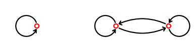
Figure 2. The weighted graph $X(v)$ associated to $v\in V_{A}$, where $v_{3}=v_{1}-(\alpha_{1}v_{2}+\alpha_{2}v_{5})/(\alpha_{1}+\alpha_{2})$ is necessarily non-negative.

The cone $V_{A}$ has four extremal vectors $\xi_{i}$ in $(v_{1},v_{2},v_{3},v_{5})$ co-ordinates, which are the columns of the matrix

$$M_{A}:=\begin{pmatrix}0&0&1&\alpha_{1}\\ -\alpha_{2}&0&0&\alpha_{1}+\alpha_{2}\\ 0&-\alpha_{2}&1&0\\ \alpha_{1}&\alpha_{1}+\alpha_{2}&0&0\\ \end{pmatrix}$$

By our assumption of the $\alpha_{i}$, the entries of this matrix are non-negative (as they must be). Note that these four vectors are linearly dependent, and $V_{A}$ is the cone on a planar quadrilateral. The cone $V_{A}$ is the image of the non-negative orthant in $\mathbb{R}^{4}$ under multiplication on the left by $M_{A}$.

A nonzero nonnegative vector $(v_{1},v_{2},v_{3},v_{5})$ is a disk vector if and only if it is integral, if $v_{1}=0$, and if $v_{3}=-(\alpha_{1}v_{2}+\alpha_{2}v_{5})/(\alpha_{1}+\alpha_{2})>0$. Since we are assuming $\alpha_{1}+\alpha_{2}>0$, the disk vectors are all contained in the face of $V_{A}$ spanned by $\xi_{1}$ and $\xi_{2}$ (i.e. the face with $v_{1}=0$). The set of disk vectors are precisely vectors of the form $(0,p,q,-(p+q)\alpha_{1}/\alpha_{2}-q)$ where $p,q$ are integers such that $q>0,p\geq 0$ and $-\alpha_{2}|p+q$. Thus the Klein polyhedron $\textnormal{conv}(\mathcal{D}_{A}+V_{A})$ has vertices $\xi_{2}$ and $d=(0,-1-\alpha_{2},1,\alpha_{1}-1)$.

The Klein polyhedron has three faces which are not contained in faces of $V_{A}$. The first face $K_{1}$ has vertex $\xi_{2}$, and has extremal rays $\xi_{2}+t\xi_{3}$ and $\xi_{2}+t\xi_{4}$ for $t\geq 0$. The second face $K_{2}$ has vertices $\xi_{2}$ and $d$, and has extremal rays $\xi_{2}+t\xi_{4}$ and $d+t\xi_{4}$, as well as the interval from $\xi_{2}$ to $d$. The third face $K_{3}$ has vertex $d$ and extremal rays $d+t\xi_{4}$ and $d+t\xi_{1}$. The Klein function $\kappa_{A}$ has the form

$$\kappa_{A}=\begin{cases}\frac{1}{\alpha_{2}}\left(v_{1}-\alpha_{1}v_{2}/(\alpha_{1}+\alpha_{2})-v_{3}\right)&\text{on the cone of }K_{1}\\ \frac{1}{\alpha_{2}}\left((\alpha_{1}+\alpha_{2})v_{1}/\alpha_{1}-v_{2}-v_{3}\right)&\text{on the cone of }K_{2}\\ v_{3}&\text{on the cone of }K_{3}\\ \end{cases}$$

while on all of $V_{A}$ we have $|v|/2=(v_{2}+2v_{3}+v_{5})/2$.

By the symmetry of $w_{\alpha,\beta}$, we obtain similar expressions for a typical vector $(u_{1},u_{2},u_{3},u_{4},u_{5})$ in $V_{B}$. With this notation, the polyhedron $Y$ is the subspace of $V_{A}\times V_{B}$ consisting of vectors for which $u_{2}=v_{2},u_{3}=v_{3},u_{4}=v_{4}$ and $u_{5}=v_{5}$. The two Abelian loops themselves impose no pairing conditions, but since we can write both $u_{1}$ and $v_{1}$ in terms of the other $u_{i},v_{i}$ (in the same way), the equalities above imply $u_{1}=v_{1}$.

Setting $d(y)=[w_{\alpha,\beta}]$ imposes two more conditions on the vectors (at first glance it looks like it imposes four conditions since there are four terms in $w$, but two of these conditions are already implicit in $v_{3}=v_{4}$ and $u_{3}=u_{4}$ which were consequences of $\partial=0$). These two extra conditions take the form $v_{2}=v_{5}$ and $v_{3}=1-v_{2}$.

The two conditions give $v_{1}=1$, $v_{2}=v_{5}=x$ and $v_{3}=1-x$. Making these substitutions, we find that $Y_{[w]}$ is the polygon $0\leq x\leq 1$.

To compute scl we must maximize $\chi$ on $Y_{[w]}$. In terms of $x$, the function $\chi$ is equal to $\kappa_{A}+\kappa_{B}-2$ where

$$\kappa_{A}=\begin{cases}x/(\alpha_{1}+\alpha_{2})&\text{if }x\leq(\alpha_{1}+\alpha_{2})/\alpha_{1}\\ 1/\alpha_{1}&\text{if }(\alpha_{1}+\alpha_{2})/\alpha_{1}\leq x\leq(\alpha_{1}-1)/\alpha_{1}\\ 1-x&\text{if }x\geq(\alpha_{1}-1)/\alpha_{1}\\ \end{cases}$$

and similarly for $\kappa_{B}$:

$$\kappa_{B}=\begin{cases}x/(\beta_{1}+\beta_{2})&\text{if }x\leq(\beta_{1}+\beta_{2})/\beta_{1}\\ 1/\beta_{1}&\text{if }(\beta_{1}+\beta_{2})/\beta_{1}\leq x\leq(\beta_{1}-1)/\beta_{1}\\ 1-x&\text{if }x\geq(\beta_{1}-1)/\beta_{1}\\ \end{cases}$$

Then $\textnormal{scl}(w)=1-\max(\kappa_{A}(x)+\kappa_{B}(x))/2$.

Proposition 4.3.

Let $w=a^{-\alpha_{1}-\alpha_{2}}+b^{-\beta_{1}-\beta_{2}}+a^{\alpha_{1}}b^{\beta_{1}}+a^{\alpha_{2}}b^{\beta_{2}}$ where the $\alpha_{i}$ and coprime and similarly for the $\beta_{i}$, and they satisfy

$$\alpha_{1}>\alpha_{1}+\alpha_{2}>0>\alpha_{2},\quad\beta_{1}>\beta_{1}+\beta_{2}>0>\beta_{2}$$

We have the following formulae for $\textnormal{scl}(w)$ by cases:

1. If $(\alpha_{1}-1)/\alpha_{1}\leq(\beta_{1}+\beta_{2})/\beta_{1}$ then $\textnormal{scl}(w)=1-\frac{1}{2}\left(\frac{1}{\alpha_{1}}+\frac{(\alpha_{1}-1)}{\alpha_{1}(\beta_{1}+\beta_{2})}\right)$

2. If $(\beta_{1}-1)/\beta_{1}\leq(\alpha_{1}+\alpha_{2})/\alpha_{1}$ then $\textnormal{scl}(w)=1-\frac{1}{2}\left(\frac{1}{\beta_{1}}+\frac{(\beta_{1}-1)}{\beta_{1}(\alpha_{1}+\alpha_{2})}\right)$

3. Otherwise $\textnormal{scl}(w)=1-\frac{1}{2}\left(\frac{1}{\alpha_{1}}+\frac{1}{\beta_{1}}\right)$

Remark 4.4.

The program scallop (see [10]) implements an algorithm described in [8] § 4.1.7–8 to compute scl on individual chains in $B_{1}^{H}(F_{2})$, and can be used to give an independent check of Proposition 4.3.

Without much more work, we can also treat chains of the form

$$w^{\prime}_{\alpha,\beta}=a^{-\alpha_{1}-\alpha_{2}}+b^{-\beta_{1}-\beta_{2}}+a^{\alpha_{1}}b^{\beta_{1}}a^{\alpha_{2}}b^{\beta_{2}}$$

The cones $V_{A},V_{B}$ are the same but now the polyhedron $Y$ is slightly different, defined by $u_{2}=v_{3}=u_{4}$ and $v_{2}=u_{3}=v_{4}$. Hence, in terms of the variable $x$, the function $\kappa_{A}$ is as before, whereas $\kappa_{B}$ has the form:

$$\kappa_{B}=\begin{cases}x&\text{if }x\leq 1/\beta_{1}\\ 1/\beta_{1}&\text{if }1/\beta_{1}\leq x\leq-\beta_{2}/\beta_{1}\\ (1-x)/(\beta_{1}+\beta_{2})&\text{if }x\geq-\beta_{2}/\beta_{1}\\ \end{cases}$$

Hence we have

Proposition 4.5.

Let $w^{\prime}=a^{-\alpha_{1}-\alpha_{2}}+b^{-\beta_{1}-\beta_{2}}+a^{\alpha_{1}}b^{\beta_{1}}a^{\alpha_{2}}b^{\beta_{2}}$ where the $\alpha_{i}$ and coprime and similarly for the $\beta_{i}$, and they satisfy

$$\alpha_{1}>\alpha_{1}+\alpha_{2}>0>\alpha_{2},\quad\beta_{1}>\beta_{1}+\beta_{2}>0>\beta_{2}$$

We have the following formulae for $\textnormal{scl}(w)$ by cases:

1. If $-\beta_{2}/\beta_{1}\leq(\alpha_{1}+\alpha_{2})/\alpha_{1}$ then

   $$\textnormal{scl}(w^{\prime})=1-\frac{1}{2}\left(\max\left(\frac{1}{\beta_{1}}-\frac{\beta_{2}}{\beta_{1}(\alpha_{1}+\alpha_{2})},\frac{1}{\alpha_{1}}-\frac{\alpha_{2}}{\alpha_{1}(\beta_{1}+\beta_{2})}\right)\right)$$

2. Otherwise $\textnormal{scl}(w^{\prime})=1-\frac{1}{2}\left(\frac{1}{\alpha_{1}}+\frac{1}{\beta_{1}}\right)$

The distribution of values of scl for all $w,w^{\prime}$ with $\alpha_{1},\beta_{1}\leq 35$ (about $3$ million words) is illustrated in Figure 3.

2pt $0$ at 0 -15 $\frac{1}{2}$ at 300 -15 $1$ at 600 -15 $\frac{1}{3}$ at 200 -15 $\frac{2}{3}$ at 400 -15 $\frac{1}{4}$ at 150 -15 $\frac{3}{4}$ at 450 -15 $\frac{1}{5}$ at 120 -15 $\frac{2}{5}$ at 240 -15 $\frac{3}{5}$ at 360 -15 $\frac{4}{5}$ at 480 -15 $\frac{1}{6}$ at 100 -15 $\frac{5}{6}$ at 500 -15 $\frac{1}{7}$ at 85.7142857 -15 $\frac{2}{7}$ at 171.42857 -15 $\frac{3}{7}$ at 257.142857 -15 $\frac{4}{7}$ at 342.85714 -15 $\frac{5}{7}$ at 428.571428 -15 $\frac{6}{7}$ at 514.285714 -15

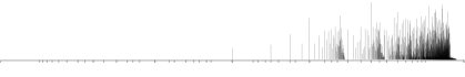
Figure 3. Histogram of values of scl on $w,w^{\prime}$

This statement about integral chains in $F_{2}$ can be translated into a statement about elements of the commutator subgroup of $F_{4}$.

Let $a,b,c,d$ be generators for a free group $F_{4}$. For each $\alpha,\beta$ define

$$w^{\prime\prime}_{\alpha,\beta}=a^{-\alpha_{1}-\alpha_{2}}cb^{-\beta_{1}-\beta_{2}}c^{-1}da^{\alpha_{1}}b^{\beta_{1}}a^{\alpha_{2}}b^{\beta_{2}}d^{-1}$$

By the self-product formula, i.e. Theorem 2.101 from [8] (also see Remark 2.102), we have an equality

$$\textnormal{scl}_{F_{4}}(w^{\prime\prime}_{\alpha,\beta})=\textnormal{scl}_{F_{2}}(w^{\prime}_{\alpha,\beta})+1$$

Consequently, by the multiplicativity of scl under taking powers, we deduce the following theorem:

Theorem 4.6 (Denominators).

The image of a nonabelian free group of rank at least $4$ under scl in $\mathbb{R}/\mathbb{Z}$ is precisely $\mathbb{Q}/\mathbb{Z}$.

If $F_{1}$, $F_{2}$ are free groups containing elements $w_{1}$ and $w_{2}$ respectively, then by the free product formula, i.e. Theorem 2.93 from [8], we have an equality $\textnormal{scl}(w_{1}w_{2})=\textnormal{scl}(w_{1})+\textnormal{scl}(w_{2})+1/2$ where the product on the left hand side is taken in the free group $F_{1}*F_{2}$. Suppose $w_{i}$ is an infinite family of elements in $F$ for which the set of numbers $\textnormal{scl}(w_{i})$ is well-ordered with ordinal type $\omega$. Then we can take two copies $F_{1},F_{2}$ of $F$, and corresponding elements $w_{i,1},w_{i,2}$ in each copy, and observe that the set of numbers $\textnormal{scl}(w_{i,1}w_{j,2})$ is well-ordered with ordinal type $\omega^{2}$. Repeating this process inductively, we deduce the following theorem:

Theorem 4.7 (Limit values).

For each $n$, the image of the free group $F_{n}$ under scl contains a well-ordered sequence of values with ordinal type $\omega^{\lfloor n/4\rfloor}$. The image of $F_{\infty}$ under scl contains a well-ordered sequence of values with ordinal type $\omega^{\omega}$.

To obtain stronger results, it is necessary to understand how $\chi$ varies as a function of the parameters in a more general surgery family.

4.2. Faces and signatures

We recall the method to compute $\textnormal{scl}(w)$ described in § 3 for a chain $w\in B_{1}^{H}(A*B)$. In broad outline, the method has three steps:

1. Construct the polyhedra $V_{A}$ and $V_{B}$ and $Y_{w}\subset V_{A}\times V_{B}$

2. Express $\chi$ as the minimum of a finite family of rational linear functions

3. Maximize $\chi$ on $Y_{w}$

In principle, step (1) is elementary linear algebra. However in practice, even for simple $w$ the polyhedra $V_{A},V_{B},Y_{w}$ become difficult to work with directly, and it is useful to have a description of these polyhedra which is as simple as possible; we take this up in § 4.3.

Given $Y_{w}$ and $\chi$, step (3) is a straightforward linear programming problem, which may be solved by any number of standard methods (e.g. Dantzig’s simplex method [11], Karmarkar’s projective method [15] and so on). These methods are generally very rapid and practical.

The “answers” to steps (1) and (3) depend piecewise rationally linearly on the parameters of the problem, and it is easy to see their contribution to scl on families obtained by a line of surgeries.

The most difficult step, and the most interesting, is (2): obtaining an explicit description of $\chi$ as a function of a parameter $p$ in a line of surgeries. Because of Proposition 3.21, this amounts to the determination of the respective Klein functions $\kappa$ on each of $V_{A}$ and $V_{B}$. This turns out to be a very difficult question to answer precisely, but we are able to obtain some qualitative results.

For a given combinatorial type of $V_{A}$, it takes a finite amount of data to specify the set of open faces with connected support (i.e. those faces with the property that the integer lattice points they contain are disk vectors). We call this data that signature of $V_{A}$, and denote in $\textnormal{sign}(V_{A})$. Evidently the sail of $V_{A}$ depends only on $\textnormal{sign}(V_{A})$ (a finite amount of data), and the orbit of $V_{A}$ under $\textnormal{GL}(C_{2}(A),\mathbb{Z})$.

4.3. Combinatorics of $V_{A}$

In this section we will give an explicit description of $V_{A}$ as a polyhedron depending on $w$. Recall that $V_{A}$ is the set of non-negative vectors in $C_{2}(A)$ in the kernel of both $\partial$ and $h$. Define $W_{A}$ to be the set of non-negative vectors in $C_{2}(A)$ in the kernel of $\partial$. Hence $V_{A}=W_{A}\cap\ker(h)$. We first give an explicit description of $W_{A}$.

Let $\Sigma$ denote the directed graph with vertex set $T(A)$ and edge set $T_{2}(A)$. Non-negative vectors in $C_{2}(A)$ correspond to simplicial $1$-chains, whose simplices are all oriented compatibly with the orientation on the edges of $\Sigma$. A vector is in the kernel of $\partial$ if and only if the corresponding chain is a $1$-cycle. Hence we can think of $W_{A}$ as a rational convex polyhedral cone in the real vector space $H_{1}(\Sigma)$.

A $1$-cycle in $H_{1}(\Sigma)$ is determined by the degree with which it maps over every oriented edge of $\Sigma$. A $1$-cycle $\phi$ in $W_{A}$ determines an oriented subgraph $\Sigma(\phi)$ of $\Sigma$ which is the union of edges over which it maps with strictly positive degree.

Lemma 4.8.

An oriented subgraph of $\Sigma$ is of the form $\Sigma(\phi)$ for some $\phi\in W_{A}$ if and only if every component is recurrent; i.e. it contains an oriented path from every vertex to every other vertex.

Proof.

For simplicity restrict attention to one component. A connected oriented graph is recurrent if and if it contains no dead ends: i.e. partitions of the vertices of $\Sigma$ into nonempty subsets $Z_{1},Z_{2}$ such that every edge from $Z_{1}$ to $Z_{2}$ is oriented positively. Since $\phi$ is a cycle, the flux through every vertex is zero. If there were a dead end $Z_{1},Z_{2}$ the flux through $Z_{2}$ would be positive, which is absurd. Hence $\Sigma(\phi)$ is recurrent.

Conversely, suppose $\Gamma$ is recurrent. For each oriented edge $e$ in $\Gamma$, choose an oriented path from the endpoint to the initial point of $e$ and concatenate it with $e$ to make an oriented loop. The sum of these oriented loops is a $1$-cycle $\phi$ for which $\Sigma(\phi)=\Gamma$. ∎

Lemma 4.8 implies that the faces of $W_{A}$ are in bijection with the recurrent subgraphs $\Gamma$ of $\Sigma$. The dimension of the face corresponding to a graph $\Gamma$ is $\dim(H_{1}(\Gamma))$. As a special case, we obtain the following:

Lemma 4.9.

The extremal rays of $W_{A}$ are in bijection with oriented embedded loops in $\Sigma$.

Example 4.10.

Given a graph $\Gamma$ (directed or not), there is a natural graph $O(\Gamma)$ whose vertices are embedded oriented loops in $\Gamma$, and whose edges are pairs of oriented loops whose union has $\dim(H_{1})=2$. In the case that $\Gamma$ is the $1$-skeleton of a tetrahedron, the graph $O(\Gamma)$ is the $1$-skeleton of a stellated cube; see Figure 4.

2pt

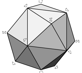
Figure 4.

The polyhedron $W_{A}$ depends only weakly on the precise form of $w$. In fact, discounting Abelian loops, the polyhedron $W_{A}$ only depends on the cardinality of $T(A)$. To describe $V_{A}$ we need to consider the function $h:C_{2}(A)\to A$. Recall that $h(\tau,\tau^{\prime})=(\tau+\tau^{\prime})/2$ where we identify elements of $T(A)$ with elements of $A$ by thinking of the $T(A)$ as loops in a $K(A,1)$. Denote this identification map by $i:T(A)\to A$ and think of $i$ as a function on the vertices of $\Sigma$, so that if $\phi$ is an embedded loop in $\Sigma$, then $h(\phi)=\sum_{v\in\phi}i(v)\in A$. Since by hypothesis $w\in B_{1}^{H}(F)$, we have $h(\phi)=0$ whenever $\phi$ is a Hamiltonian circuit (an embedded loop which passes through each vertex exactly once). Moreover for generic $w\in B_{1}^{H}(F)$ and generic $i$, these are the only embedded loops with $h=0$. In any case, we obtain a concrete description of $V_{A}$, or, equivalently, of the set of extremal rays.

Lemma 4.11.

Rays of $V_{A}$ are in the projective class of two kinds of $1$-cycles:

1. embedded oriented loops $\phi$ in $\Sigma$ with $h(\phi)=0$ (which includes the Hamiltonian circuits in $\Sigma$)

2. those of the form $h(\phi^{\prime})\phi-h(\phi)\phi^{\prime}$ where $\phi,\phi^{\prime}$ are distinct embedded oriented loops whose intersection is connected (and possibly empty), with $h(\phi^{\prime})>0$ and $h(\phi)<0$

Proof.

The rays of $V_{A}$ are the intersection of the hyperplane $h=0$ with the rays and $2$-dimensional faces of $W_{A}$. The rays of $W_{A}$ which satisfy $h=0$ are exactly the projective classes of the oriented loops $\phi$ with $h(\phi)=0$. The $2$-dimensional faces of $W_{A}$ correspond to the recurrent subgraphs $\Gamma$ with $\dim(H_{1}(\Gamma))=2$. By Mayer-Vietoris, such a $\Gamma$ is the union of a pair of embedded loops $\phi,\phi^{\prime}$ whose (possibly empty) intersection is connected. The hyperplane $h=0$ intersects such a face in a ray in the projective class of $h(\phi^{\prime})\phi-h(\phi)\phi^{\prime}$. ∎

4.4. Surgery theorem

In what follows, we fix $A*B$ and a linear family of surjective homomorphisms (i.e. a line of surgeries) $\rho_{p}:A*B\to A^{\prime}*B$ where $A,A^{\prime},B$ are free Abelian, and $\textnormal{rank}(A^{\prime})=\textnormal{rank}(A)-1$. Fix $w\in B_{1}^{H}(A*B)$ and denote $w(p):=\rho_{p}(w)$.

Recall that the set of disk vectors $\mathcal{D}_{A}$ in $V_{A}$ is the union of the integer lattice points in those open faces $F$ of $V_{A}$ for which $\textnormal{supp}(F)$ is connected. In a line of surgeries, the polyhedra $V_{A}(p)$ vary in easily understood ways. For each $p$, let $M(p)$ be an integral matrix whose columns are vectors spanning the extremal rays of $V_{A}(p)$. Then $M(p)$ has the form $M(p)=N+pN^{\prime}$, where $N$ and $N^{\prime}$ are fixed integral matrices, depending only on $w$. As $p\to\infty$, the cones $V_{A}(p)$ converge in the Hausdorff topology to a rational cone $V_{A}^{\prime}(\infty)$ spanned by the nonzero columns of $N^{\prime}$, and the columns of $N$ corresponding to the zero columns of $N^{\prime}$. The cone $V_{A}(\infty)$ associated to $w$ has codimension one in each $V_{A}(p)$, and codimension one in the limit $V_{A}^{\prime}(\infty)$.

For each $p$, let $\mathcal{D}_{A}(p)$ denote the disk vectors in $V_{A}(p)$, and $\mathcal{D}_{A}(\infty)$ the disk vectors in $V_{A}(\infty)$. Similarly, let $\kappa_{p}$ denote the Klein function on $V_{A}(p)$, and $\kappa_{\infty}$ the Klein function on $V_{A}(\infty)$. Observe that any $v$ that is in $\mathcal{D}_{A}(p)$ for some $p$ is also in $\mathcal{D}_{A}(q)$ for all $q$ such that $v$ is in $V_{A}(q)$ (i.e. the property of being a disk vector does not depend on $p$).

Lemma 4.12.

There is convergence in the Hausdorff topology

$$\textnormal{conv}(\mathcal{D}_{A}(p)+V_{A}(p))\to\textnormal{conv}(\mathcal{D}_{A}(\infty)+V_{A}^{\prime}(\infty))$$

Hence $\kappa_{\infty}=\lim_{p\to\infty}\kappa_{p}|_{V_{A}(\infty)}$.

Proof.

The set of integer lattice points is discrete. Since every integer lattice point is either in every $V_{A}(p)$ or in only finitely many, the intersection of $\mathcal{D}_{A}(p)$ with any compact subset of $W_{A}$ is eventually equal to the intersection of this compact set with $\cap_{p}\mathcal{D}_{A}(p)$. Since $V_{A}(\infty)=\cap_{p}V_{A}(p)$, we have $\mathcal{D}_{A}(\infty)=\cap_{p}\mathcal{D}_{A}(p)$.

The last claim follows because

$$\textnormal{conv}(\mathcal{D}_{A}(\infty)+V_{A}^{\prime}(\infty))\cap V_{A}(\infty)=\textnormal{conv}(\mathcal{D}_{A}(\infty)+V_{A}(\infty))$$

∎

From this discussion we derive the following theorem.

Theorem 4.13 (Surgery).

Fix $w\in B_{1}^{H}(A*B)$ and let $\rho_{p}:A*B\to A^{\prime}*B$ be a line of surgeries, constant on the second factor, and surjective on the first factor with $\textnormal{rank}(A^{\prime})=\textnormal{rank}(A)-1$. Define $w(p)=\rho_{p}(w)$. Then $\lim_{p\to\infty}\textnormal{scl}(w(p))=\textnormal{scl}(w)$.

Proof.

Denote $\lim_{p\to\infty}\kappa_{p}=\kappa_{\infty}^{\prime}$, thought of as a function on $V_{A}^{\prime}(\infty)$. Denote by $Y_{w}^{\prime}\subset V_{A}^{\prime}(\infty)\times V_{B}$ the limit as $p\to\infty$ of $Y_{w}(p)\subset V_{A}(p)\times V_{B}$. Since $|v_{A}|$ is constant on each $Y_{w}(p)$, it follows that $|v_{A}|$ is also constant on $Y_{w}^{\prime}$. Lemma 4.12 implies that the only disk vectors in $V_{A}^{\prime}(\infty)$ which contribute to $\kappa_{\infty}^{\prime}$ are those in $V_{A}(\infty)$. Since $|v_{A}|$ is non-negative on $V_{A}^{\prime}(\infty)$, a level set of $|v_{A}|$ which is a supporting hyperplane for $\textnormal{conv}(\mathcal{D}_{A}(\infty)+V_{A}(\infty))$ is also a supporting hyperplane for $\textnormal{conv}(\mathcal{D}_{A}(\infty)+V_{A}^{\prime}(\infty))$. It follows that $\chi$ restricted to $Y_{w}^{\prime}$ is maximized in $Y_{w}$. The result follows by applying Theorem 3.14. ∎

Remark 4.14.

By monotonicity of scl under homomorphisms one has the inequality $\textnormal{scl}(w(p))\leq\textnormal{scl}(w)$ for all $p$. Thus surgery “explains” the existence of many nontrivial accumulation points in the scl spectrum of a free group. However it should also be pointed out that equality is sometimes achieved in families, so that $\textnormal{scl}(w(p))=\textnormal{scl}(w)$ for all $p$ (for example, under the conditions discussed in Example 3.20).

It is interesting to note that the limit does not depend on the particular surgery family.

Example 4.15.

Let $w=a^{2}c^{2}ba^{-1}b^{-1}c^{-1}ba^{-1}c^{-1}b^{-1}$ where $[a,c]=\textnormal{id}$, and $b$ generates a free summand. Consider the line of surgeries defined by $\rho_{p}(a)=a$, $\rho_{p}(b)=b$ and $\rho_{p}(c)=pa$. In this case, $w(p)=a^{2+2p}ba^{-1}b^{-1}a^{-p}ba^{-1-p}b^{-1}$. Then

$$\textnormal{scl}(w(p))=\frac{4p+3}{4p+4}\text{ if }p\text{ is odd, and }\frac{2p+1}{2p+2}\text{ if }p\text{ is even.}$$

Define $\sigma=\bigl{(}\begin{smallmatrix}1&0\\ 1&1\end{smallmatrix}\bigr{)}$ and consider the line of surgeries obtained by the same homomorphisms $\rho_{p}$ precomposed with the automorphism $\sigma$ of $\mathbb{Z}^{2}$. Then

$$\textnormal{scl}(w(p)^{\sigma})=\frac{8p+3}{8p+4}\text{ if }p\text{ is odd, and }\frac{4p+5}{4p+6}\text{ if }p\text{ is even.}$$

Both sequences of numbers converge to $1=\textnormal{scl}(w)$ as $p\to\infty$. Note that even when the values of $\textnormal{scl}(w(p))$ and $\textnormal{scl}(w(q)^{\sigma})$ agree, the corresponding elements are typically not in the same Aut orbit in $F_{2}$.

Remark 4.16.

The precise algebraic form of $\textnormal{scl}(w(p))$ on surgery families is analyzed in a forthcoming paper of Calegari-Walker [9], where it is shown quite generally that $\textnormal{scl}(w(p))$ is a ratio of quasipolynomials in $p$, for $p\gg 0$.

4.5. Computer implementation

The algorithm described in this paper has been implemented by Alden Walker in the program sss, available from the author’s website [19]. This allows computations that would be infeasible with scallop; e.g. $\textnormal{scl}(aba^{-98}ba^{-1}b^{-3}+a^{98}b)=195/196$. The runtime in this implementation appears to be doubly exponential in the number of $A$ and $B$ arcs, and the practical limit for this number appears to be no more than about $5$ (excluding Abelian loops).

Some theoretical explanation for this difficulty comes from recent work of Lukas Brantner [5], who shows (amongst other things) that the problem of deciding whether a given disk vector $d\in\mathcal{D}_{A}$ is essential — i.e. cannot be written as $d=e+v$ for $e\in\mathcal{D}_{A}$ and $v\in V_{A}-0$ — is coNP-complete.

5. Acknowledgment

I would like to thank Lukas Brantner, Jon McCammond, Alden Walker and the referee for helpful comments and corrections. While writing this paper I was partially supported by NSF grants DMS 0707130 and DMS 1005246.

References

- [1] V. Arnold, Higher-dimensional continued fractions, Regul. Chaotic Dyn. 3 (1998), no. 3, 10–17
- [2] A. Barvinok, Integer Points in Polyhedra, Zurich lectures in advanced mathematics. EMS, Zurich, 2008
- [3] C. Bavard, Longueur stable des commutateurs, Enseign. Math. (2), 37, 1-2, (1991), 109–150
- [4] B. Bollobás, Modern graph theory, Springer GTM 184, Springer-Verlag, New York, 1998
- [5] L. Brantner, On the complexity of sails, preprint, in preparation
- [6] M. Burger and N. Monod, On and around the bounded cohomology of , Rigidity in dynamics and geometry (Cambridge, 2000), Springer, Berlin, 2002, 19–37
- [7] D. Calegari, Stable commutator length is rational in free groups, Jour. AMS, 22 (2009), no. 4, 941–961
- [8] D. Calegari, scl, MSJ Memoirs, 20. Mathematical Society of Japan, Tokyo, 2009
- [9] D. Calegari and A. Walker, Integer hulls of linear polyhedra and scl in families, preprint, in preparation
- [10] D. Calegari and A. Walker, scallop, computer program, available from the authors’ websites
- [11] G. Dantzig, Linear Programming and Extensions, Princeton Univ. Press, Princeton, 1963
- [12] D. Gabai, Foliations and the topology of -manifolds, J. Diff. Geom. 18 (1983), no. 3, 445–503
- [13] P. Gordan, Über die Auflösung linearer Gleichungen mit reelen Coefficienten, Math. Ann. 6, (1873), 23–28
- [14] M. Gromov, Volume and bounded cohomology, Inst. Hautes Études Sci. Publ. Math. No. 56 (1982), 5–99
- [15] N. Karmarkar, A new polynomial-time algorithm for linear programming, Combinatorica 4 (1984), no. 4, 373–395
- [16] F. Klein, Über eine geometrische Auffassung der gewöhnlichen Kettenbruchentwicklung, Nachr. Ges. Wiss. Göttingen, Math.-Phys. 3, (1895), 357–359
- [17] S. Mac Lane, Homology, Springer classics in mathematics, Berlin, 1995
- [18] J. Stallings, Surfaces mapping to wedges of spaces. A topological variant of the Grushko-Neumann theorem, Groups—Korea ’98 (Pusan), 345–353, de Gruyter, Berlin, 2000
- [19] A. Walker, sss, computer program, available from the author’s website
- [20] D. Zhuang, Irrational stable commutator length in finitely presented groups, J. Mod. Dyn. 2 (2008), no. 3, 499–507