Extrapolated High-Order Propagators for Path Integral Monte Carlo Simulations

Abstract

We present a new class of high-order imaginary time propagators for path-integral Monte Carlo simulations by subtracting lower order propagators. By requiring all terms of the extrapolated propagator be sampled uniformly, the subtraction only affects the potential part of the path integral. The negligible violation of positivity of the resulting path integral at small time steps has no discernable affect on the accuracy of our method. Thus in principle arbitrarily high order algorithms can be devised for path-integral Monte Carlo simulations. We verify this claim is by showing that fourth, sixth, and eighth order convergence can indeed be achieved in solving for the ground state of strongly interacting quantum many-body systems such as bulk liquid ⁴He.

I Introduction

Many quantum Monte Carlo (QMC) techniques, such as path integral [ground state] Monte Carlo (PI[GS]MC) and diffusion Monte Carlo (DMC), rely on stochastic propagation of the Schrödigner equation in imaginary time. In all these methods, the probability distribution sampled is the matrix element, or the trace, of the imaginary time propagator

$$G(\tau)={\rm e}^{-\tau H}={\rm e}^{-\tau(T+V)},$$ (1)

with Hamiltonian $H=T+V$ and kinetic and potential operators $T=(-\hbar^{2}/2m)\sum_{i}\nabla^{2}_{i}$ and $V=\sum_{i<j}v(r_{ij})$. Since $G(\tau)$ is generally unknown, $\tau$ is usually discretized into a sum of short time steps $\epsilon$ so that the full propagator $G(\epsilon)$ can be approximated by a product of short-time approximate propagator $\tilde{G}(\epsilon)$. The computational effort, and therefore the efficiency of these QMC techniques depends on $\epsilon$. If $\tilde{G}(\epsilon)$ is accurate to high orders in $\epsilon$, then a large $\epsilon$ can be used to span a given imaginary time interval, resulting in fewer samplings of (but possibly more complex) $\tilde{G}(\epsilon)$.

For QMC simulations, there is a surprise lack of general higher order algorithms. For example, one has the well known second-order, primitive propagator

$$G_{2}(\epsilon)={\rm e}^{-\epsilon V/2}{\rm e}^{-\epsilon T}{\rm e}^{-\epsilon V/2}=G(\epsilon)+{\rm O}(\epsilon^{3}).$$ (2)

(For computing the trace, any splitting first-order algorithm, such as ${\rm e}^{-\epsilon V}{\rm e}^{-\epsilon T}$, will also yield a second-order tracechin04 .) The highly successful pair density propagator, that approximates $G$ by a pair-wise product of exact two-body propagators ceperleyRMP95 must also be second order in the general many-particle case, but possibly with a small error coefficient. However, this approach in practice is limited to solely spherically symmetric interactions due to the difficulty of evaluating the two-particle density matrix exactly. The only fourth-order method known for many years is the Takahashi-Imadati , Li-Broughtonli propagator

$$G_{\rm TI}(\epsilon)={\rm e}^{-\epsilon T/2}e^{-\epsilon V-(\epsilon^{3}/24)[V,[T,V]]}e^{-\epsilon T/2}=G(\epsilon)+{\rm O}(\epsilon^{3})\,,$$ (3)

where $[V,[T,V]]=\frac{\hbar^{2}}{m}\sum_{i}|\nabla_{i}V|^{2}$. This “corrector” propagator is only second order, but yields a fourth-order trace, as explained in Ref.chin04, . Thus until recently, there were only two second-order and one fourth-order algorithm for PIMC simulations.

The problem of constructing higher order PIMC algorithms is the time-irreversible nature of the imaginary time Schrödinger equation. The short-time propagator can in general be approximated to any order by a product decomposition,

$${\rm e}^{-\epsilon(T+V)}\approx\prod_{i=1}^{N}{\rm e}^{-t_{i}\epsilon T}{\rm e}^{-v_{i}\epsilon V},$$ (4)

with coefficients $\{t_{i},v_{i}\}$ determined by the required order of accuracy. However, in QMC applications, since $\langle R^{\prime}|\,{\rm e}^{-t_{i}\epsilon T}|\,R\rangle\propto{\rm e}^{-(R^{\prime}-R)^{2}/(4Dt_{i}\epsilon)}$ is the diffusion kernel with $D={\hbar^{2}/2m}$, the coefficient $t_{i}$ must be positive in order for the kernel to be normalizable as a probability distribution. As first proved by Shengsheng and Suzukisuzukinogo , and later by Goldman-Kapergoldman and Chinchin063 , beyond second order, any factorization of the form (4) must contain some negative coefficients in the set $\{t_{i},v_{i}\}$. Thus, despite myriad of higher-order propagators of the single product form (4) for solving the time-reversible, real-time Schrödinger equation, none can be applied in PIMC beyond second order. It is only in the last decade that bona fide fourth order, forward algorithms with all positive coefficients have been foundsuzfour ; chin97 and applied to DMC and PIMC simulationsfchinl ; fchinm ; jang . In order to circumvent the Sheng-Suzuki theorem, one must include the operator $[V,[T,V]]$ in the factorization process. Unfortunately, it not possible to go beyond fourth-order by including more operators. It has been shownchin051 that a forward sixth-order propagator would have required the operator $[V,[T,[T,[T,V]]]]$, which is non-separable and impractical to implement. More recently, by fine-tuning a family of fourth-order forward algorithm with two free parameterschinchen02 such that the fourth-order error is zero, Sakkos, J. Casulleras and J. Boronatcasulleras , and later also one of usmayrhoferDiplom , have achieved sixth-order convergence in computing the energy of a number of quantum systems including liquid ⁴He. Despite this spectacular advance, it must be noted that the fine-tuning must be done, in principle, for each individual observable. The algorithm is therefore only “quasi-sixth-order” rather than uniformly sixth-order.

In this paper, we will present the first QMC simulations using a bona fide sixth-order and eighth-order algorithm for imaginary time propagation. The algorithm is based on the multi-product expansionchin084 of the short time propagator, which is a new way of achieving higher order convergence circumventing the Sheng-Suzuki theorem. This is reviewed in Section II.1 followed by a brief introduction to path integral ground state Monte Carlo (PIGSMC) in section II.2.

II Theory

II.1 Multi-product expansion of $G$

Let $G_{2}(\epsilon)$ denote the second-order split propagator (2), then for a given set of $n$ whole numbers $\{k_{i}\}$, the multi-product expansion of Ref.chin084, yields the following second-order propagator:

$$G_{2n}(\epsilon)=\sum_{i=1}^{n}c_{i}G_{2}^{k_{i}}(\epsilon/k_{i})=G(\epsilon)+O(\epsilon^{2n+1})$$ (5)

where the expansion coefficient has the closed form

$$c_{i}=\prod_{j=1(\neq i)}^{n}\frac{k_{i}^{2}}{k_{i}^{2}-k_{j}^{2}}.$$ (6)

For PI(GS)MC, it is convenient to choose the sequences $\{k_{i}\}=\{1,2\},\{1,2,4\}$ and $\{1,2,3,6\}$ to produce the following fourth, sixth and eighth-order propagators:

$$G_{4}(\epsilon) =-\frac{1}{3}G_{2}(\epsilon)+\frac{4}{3}G_{2}^{2}\left(\frac{\epsilon}{2}\right)$$ (7)

$$G_{6}(\epsilon) =\frac{1}{45}G_{2}(\epsilon)-\frac{4}{9}G_{2}^{2}\left(\frac{\epsilon}{2}\right)+\frac{64}{45}G_{2}^{4}\left(\frac{\epsilon}{4}\right)$$ (8)

$$G_{8}(\epsilon) =-\frac{1}{840}G_{2}(\epsilon)+\frac{2}{15}G_{2}^{2}\left(\frac{\epsilon}{2}\right)$$

$$-\frac{27}{40}G_{2}^{3}\left(\frac{\epsilon}{3}\right)+\frac{54}{35}G_{2}^{6}\left(\frac{\epsilon}{6}\right).$$ (9)

As we will see later, these sequences are chosen because they are the minimal “commensurate” sequences. Schmidt and Leekevin95 have previously suggested the use of (7) in path integrals and did use it in computing the two-particle density matrix. However, they did not suggest that it can be used for doing path integral Monte Carlo simulations.

Since $G(\epsilon)>0$, only the error terms in eq. (5) can be negative. Thus for sufficiently small $\epsilon$, these extrapolated propagators, despite the explicit subtractions, must be positive. Only when $\epsilon$ is sufficiently large, the error terms overwhelm $G(\epsilon)$ in a significant fraction of configuration space. We will see below that such large $\epsilon$ cannot be used anyway because the propagators become highly inaccurate. One might argue that the error terms can be so singular that despite the smallness of $\epsilon$, it can overwhelm $G(\epsilon)$ at some specific locations. However, this cannot happen, because by construction $G_{2}(\epsilon)$ is bounded everywhere (except in the case of the Coulomb potential, which is a well known problemli in PIMC and which we exclude from the present consideration). The subtraction of two bounded functions cannot be singular. This point will be clear when we present the explicit construction of extrapolated propagators and numerical results in the following sections.

II.2 Path integral ground state Monte Carlo

The above multi-product propagators can be applied to any general PIMC simulations. Here, we will implement it in the specific context of PIGSMC. PIGSMC samples the whole probability distribution function corresponding to a discretized imaginary time propagation from a trial wave function $\Psi_{T}(R)$ to the (in principle) exact ground state $\Psi_{0}(R)$, where $R$ denotes all degrees of freedom, e.g. for the translational coordinates of $N$ particles, $R=({\bf r}_{1},\dots,{\bf r}_{N})$.

For any trial wave function $\Psi_{T}$ with non-zero overlap with the exact ground state, the exact ground state wave function can be obtained by evolving in imaginary time

$$\Psi_{0}(R)\propto\lim_{\beta/2\rightarrow\infty}\int G(R,R^{\prime},{\frac{\beta}{2}})\Psi_{T}(R^{\prime})dR^{\prime}.$$

$G({\frac{\beta}{2}})$ is evaluated by factorizing it into a product of small time step propagators $G(\epsilon)$, $\epsilon=\frac{\beta}{2M}$, which can be approximate by one of the above-mentioned short time approximations. Therefore, the full probability distribution to be sampled is

$$P(R_{0},\dots,R_{2M})= {\frac{1}{\cal N}}\Psi_{T}(R_{0})\ G(R_{0},R_{1};\epsilon)\dots$$

$$G(R_{2M-1},R_{2M};\epsilon)\ \Psi_{T}(R_{2M}),$$

so that the expectation value $\langle\Psi_{0}|A|\Psi_{0}\rangle$ of a local operator $A(R)$ is evalutated by sampling $A$ at the central time step, $A(R_{M})$. For the energy, we take advantage of $[H,G]=0$ to obtain the energy estimator in terms of the local energy of the trial wave function $E_{L}(R)={H\Psi_{T}/\Psi_{T}}$

$$E_{0}=\int\!dR_{0}\dots dR_{2M}\ E_{L}(R_{0})\,P(R_{0},\dots,R_{2M})\,.$$

These multidimensional integrations can be carried out with the Metropolis method.

II.3 Implementing multi-product expansions in PIGSMC

To see how one can implement these multi-product propagators in PIGSMC, we will now give a detailed discussion of the fourth order case. Considering $G_{4}$ at time step size $2\epsilon$:

$$G_{4}(2\epsilon) =\frac{4}{3}{\rm e}^{-\epsilon V/2}{\rm e}^{-\epsilon T}{\rm e}^{-\epsilon V}{\rm e}^{-\epsilon T}{\rm e}^{-\epsilon V/2}$$

$$-\frac{1}{3}{\rm e}^{-\epsilon V}{\rm e}^{-2\epsilon T}{\rm e}^{-\epsilon V}.$$

In evaluating the matrix element of $G_{4}(2\epsilon)$, since the first term on the RHS has one more operator ${\rm e}^{-\epsilon T}$, it would require one more intermediate state integration than the second term, resulting in two dissimilar terms difficult to sample uniformly. The key contribution of this work is to enforce uniformity by artificially splitting the single operator ${\rm e}^{-2\epsilon T}$ in the second term into two:

$$G_{4}(2\epsilon) =\frac{4}{3}{\rm e}^{-\epsilon V/2}{\rm e}^{-\epsilon T}{\rm e}^{-\epsilon V}{\rm e}^{-\epsilon T}{\rm e}^{-\epsilon V/2}$$

$$-\frac{1}{3}{\rm e}^{-\epsilon V}{\rm e}^{-\epsilon T}{\rm e}^{-\epsilon T}{\rm e}^{-\epsilon V},$$ (10)

which gives in the coordinate respresentation

$$\langle 1|G_{4}(2\epsilon)|3\rangle=\int d2\langle 1|{\rm e}^{-\epsilon T}|2\rangle\langle 2|{\rm e}^{-\epsilon T}|3\rangle$$

$$\qquad\qquad\times\Big{[}\frac{4}{3}{\rm e}^{-\epsilon V_{1}/2-\epsilon V_{2}-\epsilon V_{3}/2}-\frac{1}{3}{\rm e}^{-\epsilon V_{1}-\epsilon V_{3}}\Big{]}$$

$$=\int d2G_{0}(12;\epsilon)G_{0}(23;\epsilon){\rm e}^{-\epsilon V_{1}/2-\epsilon V_{2}-\epsilon V_{3}/2}F(123,\epsilon)$$ (11)

where we have denoted $V_{k}=V(R_{k})$ and abbreviated $R_{k}\rightarrow k$. We have defined

$$F(123,\epsilon)=\frac{1}{3}\Big{[}4-{\rm e}^{-\epsilon\left(\frac{V_{1}+V_{3}}{2}-V_{2}\right)}\Big{]},$$ (12)

and the free propagator

$$G_{0}(12;\epsilon)=\langle 1|{\rm e}^{-\epsilon T}|2\rangle=(4\pi D\epsilon)^{-3N/2}{\rm e}^{-\frac{(R_{1}-R_{2})^{2}}{4D\epsilon}}.$$ (13)

We observe that: (i) Without the factor $F$, (11) is just accurate to second order. (ii) By including $F$, only the potential energy is extrapolated in order to convert $G$ to fourth-order. (iii) For sufficiently small $\epsilon$, $F>0$. (iv) If the potential function is mostly convex (such as Lennard-Jones type potential near the potential minimum), then one has

$$\frac{V(R_{1})+V(R_{3})}{2}\geq V\Big{(}\frac{R_{1}+R_{3}}{2}\Big{)}.$$ (14)

Since

$$G_{0}(12;\epsilon)G_{0}(23;\epsilon)=\frac{{\rm e}^{-\frac{1}{2D\epsilon}(R_{2}-\frac{R_{1}+R_{3}}{2})^{2}}}{(2\pi D\epsilon)^{3N/2}}G_{0}(13;2\epsilon),$$

for fixed $R_{1}$ and $R_{3}$, $R_{2}$ is normally distributed about $(R_{1}+R_{3})/2$ with width $\propto\sqrt{\epsilon}$. If $R_{2}$ is such that it is between $R_{1}$ and $R_{3}$, then the convexity condition (14) would guarrantee (12) to be positive for all $\epsilon$. This only fails when the width of the Gaussian distribution for $R_{2}$ exceeds $|R_{1}-R_{3}|/2$, suggesting that the near-positivity of $F$ can extend over a rather wide range of $\epsilon$, which is indeed observed. Metropolis sampling requires exact positivity of $F$, which we ensure by using $\max(0,F)$, i.e. rejecting moves where $F<0$. We also collect statistics about these rejections, so ensure that their rate is low, and decreasing with $\epsilon$.

The generalization to higher order is now clear. For the sixth-order, Eq.(8),

$$G_{6}(4\epsilon) =\frac{64}{45}{\rm e}^{-\epsilon V/2}{\rm e}^{-\epsilon T}{\rm e}^{-\epsilon V}{\rm e}^{-\epsilon T}{\rm e}^{-\epsilon V}{\rm e}^{-\epsilon T}{\rm e}^{-\epsilon V}{\rm e}^{-\epsilon T}{\rm e}^{-\epsilon V/2}$$

$$-\frac{4}{9}{\rm e}^{-\epsilon V}{\rm e}^{-\epsilon T}{\rm e}^{-\epsilon T}{\rm e}^{-2\epsilon V}{\rm e}^{-\epsilon T}e^{-\epsilon T}{\rm e}^{-\epsilon V}$$

$$+\frac{1}{45}{\rm e}^{-2\epsilon V}{\rm e}^{-\epsilon T}{\rm e}^{-\epsilon T}{\rm e}^{-\epsilon T}{\rm e}^{-\epsilon T}{\rm e}^{-2\epsilon V},$$ (15)

yielding the coordinate representation

$$G_{6}(12345;4\epsilon) =G_{0}(12;\epsilon)G_{0}(23;\epsilon)G_{0}(34;\epsilon)G_{0}(45;\epsilon)$$

$$\times\Big{[}\frac{64}{45}{\rm e}^{-\epsilon V_{1}/2-\epsilon V_{2}-\epsilon V_{3}-\epsilon V_{4}-\epsilon V_{5}/2}$$

$$-\frac{4}{9}{\rm e}^{-\epsilon V_{1}-2\epsilon V_{3}-\epsilon V_{5}}+\frac{1}{45}{\rm e}^{-2\epsilon V_{1}-2\epsilon V_{5}}\Big{]}.$$ (16)

Similarly for the eighth-order (9),

$$G_{8}(1234567;6\epsilon)=G_{0}(12;\epsilon)G_{0}(23;\epsilon)\dots G_{0}(67;\epsilon)$$

$$\times\Bigl{[}\frac{54}{35}{\rm e}^{-\epsilon V_{1}/2}{\rm e}^{-\epsilon V_{2}}{\rm e}^{-\epsilon V_{3}}{\rm e}^{-\epsilon V_{4}}{\rm e}^{-\epsilon V_{5}}{\rm e}^{-\epsilon V_{6}}{\rm e}^{-\epsilon V_{7}/2}$$

$$-\frac{27}{40}{\rm e}^{-\epsilon V_{1}}{\rm e}^{-2\epsilon V_{3}}{\rm e}^{-2\epsilon V_{5}}{\rm e}^{-\epsilon V_{7}}$$

$$+\frac{2}{15}{\rm e}^{-3\epsilon V_{1}/2}{\rm e}^{-3\epsilon V_{4}}{\rm e}^{-3\epsilon V_{7}/2}-\frac{1}{840}{\rm e}^{-3\epsilon V_{1}}{\rm e}^{-3\epsilon V_{7}}\Bigr{]}\,.$$ (17)

For commensurate sequences one can factor out all the free-propagators and restrict the extrapolation process only to the potential energy function.

III Results

We have implemented the PIGSMC algorithm using multi-level sampling as described in the review ceperleyRMP95 . We compare our new extrapolated fourth, sixth, and eighth order propagators with the primitive (second-order) and the fourth-order forward propagatorschin97 4A

$$G_{4A}(\epsilon)={\rm e}^{-{\epsilon\over 6}V}{\rm e}^{-{\epsilon\over 2}T}{\rm e}^{-{2\epsilon\over 3}V-\frac{\epsilon^{3}}{72}[V,[T,V]]}{\rm e}^{-{\epsilon\over 2}T}{\rm e}^{-{\epsilon\over 6}V}\,.$$ (18)

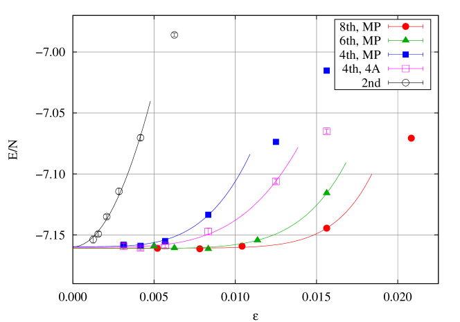
To demonstrate that our multi-product propagators work for realistic, and strongly interacting quantum systems, we apply them to the case of bulk liquid ⁴He. We calculate the ground state energy $E_{0}$ at equilibrium density $\rho_{0}=0.02186$Å^-3, by a PIGSMC simulation of 64 ⁴He atoms in a simulation box with periodic boundary conditions. The decay time is $\beta=0.25$K^-1, and we use the potential by Aziz et al. aziz79 . In Fig. 1 we show $E_{0}/N$ as function of $\epsilon$ for various propagators. We fit the polynomial $a+b\epsilon^{n}$ (lines) to $E_{0}(\epsilon)/N$, where $n$ is the order of the respective propagator. Since the order of $E_{0}(\epsilon)$ is defined as the $\epsilon\to 0$ behavior, we have restricted the fits to small values of $\epsilon$ – the end point of the lines indicate the fitting interval. These propagators are compared at equal time steps: $G_{2}(\epsilon)$, $G_{4}(\epsilon)$, $G_{6}(\epsilon)$, and $G_{8}(\epsilon)$, to verify the order of convergence.

The primitve second-order propagator (open circle) is clearly a poor approximation, with a large error even for small $\epsilon$, and therefore requires a large number of beads. The simplest fourth-order forward propagator 4A, Eq.(18), is a significant improvement, as can be seen in the behavior of $E_{0}(\epsilon)/N$ (open square), with error coefficient smaller than our fourth-order multi-product propagator (11) (filled square). However, the forward 4A propagator requires the the computation of $[V,[T,V]]\propto|\nabla_{i}V|^{2}$, and its relative efficiency would depend on the complexity of evaluating this gradient. Both can be fitted well by a fourth-order polynomial with $n=4$. Finally, the closed triangle and circle show the convergence of the sixth order (16) and eighth order (17) multi-product expansion, which indeed has a smaller $\epsilon$ dependence in the range of Fig. 1. These multi-product propagators are true high order propagators and will produce sixth and eighth order convergence for the expectation value of any observable. The present results constitute the first implementation of a quantum Monte Carlo simulation with a bona fide imaginary time propagator of higher than fourth order. At small values of the time step size, say at $\epsilon=0.005$, the sixth and eighth order algorithms produce very precise results which are not indicated by Fig.1.

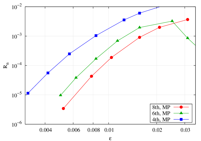
The multi-product expansion of $G$, Eq. (5), is not strictly positive everywhere for a finite time step $\epsilon$, as we have discussed above for the fourth-order case. In Fig. 2 we show the ratio $R_{n}$ of attempted MC moves that are rejected due to negativity of the multiproduct expansion. $R_{n}$ is decreasing with $\epsilon$ as expected. Only in the sixth-order case that we observed a non-monotonous behavior at very large $\epsilon$, that the ratio $R_{n}$ decreases with increasing $\epsilon$. This occurs at large values of $\epsilon$ where the error of the energy $E_{0}(\epsilon)/N$ is rapidly increasing with $\epsilon$ (outside the range of Fig. 1). This may due to system configurations with complicated intertwining negative and positive regions of $G$. We want to stress that, since this happens only for $\epsilon$ much too large for quantitatively correct results, it poses no practical limitations.

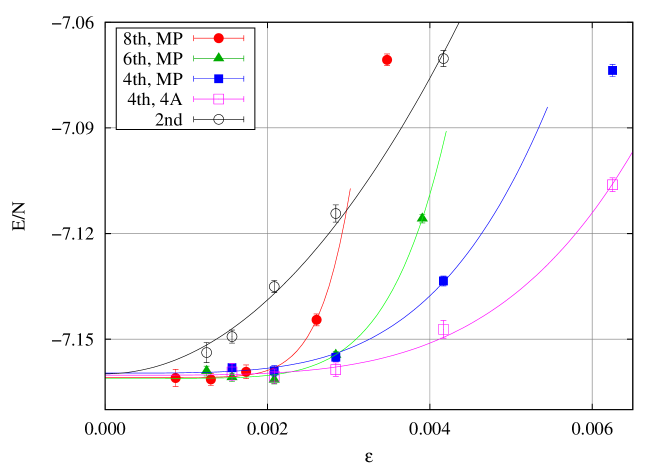
The convergence plot Fig. 1 does not reveal the actual computational effort required for a desired accuracy. From our derivation, it is clear that the computational effort of $G_{4}$, $G_{6}$, and $G_{8}$ are roughly equivalent to running $G_{2}$ twice, four, and six times, respectively. This then means that for a given $\epsilon$ for $G_{2}(\epsilon)$, one should compare it to $G_{4}$ at $2\epsilon$, $G_{6}$ at $4\epsilon$ and $G_{8}$ at $6\epsilon$, that is, for an equal effort comparison, we should compare $G_{2}(\epsilon)$, $G_{4}(2\epsilon)$, $G_{6}(4\epsilon)$ and $G_{8}(6\epsilon)$. This is done in Fig. 3. In this comparison, at a given $\epsilon$ each algorithm uses the same number of beads. For the forward algorithm 4A, this comparison neglects the additional cost of evaluating the gradient $|\nabla_{i}V|^{2}$. If $|\nabla_{i}V|^{2}$ required no more effort than that of evaluating the potential, then propagator 4A would actually outperform the extrapolated sixth- and eighth-order algorithms at time steps $\epsilon\gtrsim 0.003$K^-1. This confirms that, in principle, a purely forward time step algorithm can be more efficient, provide that $|\nabla_{i}V|^{2}$ can be easily evaluated. However, the higher order extrapolated algorithms are clearly easier to derive and implement. Morever, when very high accuracy is required, such the “chemical accuracy” required in quantum chemistry applications, then a higher order algorithm will always outperform a lower order algorithm. This is specially critical in determining the equilibrium configuration or conformation of clusters and macromolecules, where energy differences are very small.

IV Conclusion and Outlook

In this work, we have shown how to implement the multi-product expansion of the imaginary time propagator in QMC for solving strongly interacting quantum many-body systems, such ⁴He, to any desired order in the imaginary time step $\epsilon$. In particular this work is the first demonstration of truly sixth- and eighth-order QMC algorithms. In the case of ⁴He, our results suggest that these higher than fourth-order algorithms may not be more efficient than purely forward time step fourth-order algorithms, but they do have the simplicity of not requiring the potential gradient. This is particularly useful in simulating non-cartesian coordinate systems, such as molecules zillichJCP05 with anisotropic constituents and rotational degrees of freedom. Moreover, these extrapolated propagators are the only higher order algorithms possible in cases where the double-commutator cannot be evaluated, such as for the diatoms-in-molecule potential leinoJCP08 . Finally, for QMC applications where chemical accuracy is required, such as in determining equilibrium configurations and conformations, our sixth and higher order multi-product propagators will be computationally more efficient than fourth-order propagators.

Figure 1: (color online) Ground state energy $E_{0}$ of bulk ⁴He, simulated by 64 ⁴He atoms, as a function of imaginary time step $\epsilon$. Decay time was $\beta=0.25$K^-1. We compare results produced by the primitive second-order propagator $G_{2}(\epsilon)$ and the fourth-order forward propagatorchin97 $G_{4A}(\epsilon)$ (denoted “4A”) with our fourth, sixth, and eighth-order multi-product propagators $G_{4}(\epsilon)$, $G_{6}(\epsilon)$ and $G_{8}(\epsilon)$, (denoted “MP”). Each $E_{0}(\epsilon)$ is fitted with the appropriate polynomial.

Figure 2: (color online) The ratio $R_{n}$ of rejected MC moves that would lead to a negative propagator $G$. $R_{n}$ is decreasing with time step $\epsilon$.

Figure 3: (color online) A roughly equal effort comparison of algorithms $G_{2}(\epsilon)$, $G_{4}(2\epsilon)$, $G_{6}(4\epsilon)$, $G_{8}(6\epsilon)$ and $G_{4A}(2\epsilon)$ for the same ground state energy $E_{0}$ as in Fig. 1.