On the transient nature of localized pipe flow turbulence

Abstract

The onset of shear flow turbulence is characterized by turbulent patches bounded by regions of laminar flow. At low Reynolds numbers localized turbulence relaminarises, raising the question of whether it is transient in nature or it becomes sustained at a critical threshold. We present extensive numerical simulations and a detailed statistical analysis of the data, in order to shed light on the sources of the discrepancies present in the literature. The results are in excellent quantitative agreement with recent experiments and show that the turbulent lifetimes increase super-exponentially with Reynolds number. In addition, we provide evidence for a lower bound below which there are no meta-stable characteristics of the transients, i.e. the relaminarisation process is no longer memoryless.

1 Introduction

The development of turbulence in shear flows poses a challenge of great theoretical and practical relevance (Grossmann, 2000; Eckhardt et al., 2007). Since the seminal work of Reynolds (1883) on the onset of turbulent fluid motion in a circular pipe, this system has remained a paradigm for transition without linear instability, i.e. subcritical transition. Here, the boundary that separates the laminar flow from turbulence depends not only on the Reynolds number (Re), but also on the characteristics of ambient and external perturbations. In particular, the threshold in perturbation amplitude that must be exceeded to trigger transition scales as $\mbox{{Re}}^{-\gamma}$, with $\gamma\in[1,2]$ depending on the perturbation details (Hof, Juel & Mullin, 2003; Peixinho & Mullin, 2007; Mellibovsky & Meseguer, 2009). Thus, if great care is taken to minimize all sources of disturbances, the flow can be kept laminar up to Re as large as $10^{5}$ (Pfenniger, 1961).

Brosa (1989) showed that even long times after turbulence is initially triggered, relaminarisation to Hagen-Poiseuille flow may occur. Faisst & Eckhardt (2004) systematically studied the probability of a turbulent trajectory surviving up to time $t$, given by the survivor function

$$S(t)=P(\mbox{flow is turbulent at }T\geq t).$$ (1)

They concluded that relaminaristaion occurs suddenly and that the process is memoryless, i.e. lifetimes are exponentially distributed with $S(t)=\exp[t/\tau]$, where $\tau$ is the mean turbulent lifetime. This behavior had been previously observed in turbulent relaminarisation experiments in plane Couette flow (Bottin & Chaté, 1998; Bottin et al., 1998). The exponential distribution of lifetimes and sensitive dependence on initial conditions (Darbyshire & Mullin, 1995; Faisst & Eckhardt, 2004) is consistent with the presence of a repellor in phase space, a strange saddle (see e.g. Kerswell, 2005; Eckhardt, 2008). The skeleton of the saddle is then constructed from exact unstable solutions of the Navier–Stokes equations, and the simplest of such solutions correspond to nonlinear travelling waves, discovered numerically by Faisst & Eckhardt (2003) and Wedin & Kerswell (2004). Close visits to such travelling waves in turbulent flows were reported in the experiments of Hof et al. (2004) and simulations by Kerswell & Tutty (2007). Recently, new classes of travelling waves solutions and relative periodic orbits have also been found (Pringle & Kerswell, 2007; Duguet, Pringle & Kerswell, 2008).

Faisst & Eckhardt (2004) investigated the scaling of mean turbulent lifetimes as Re is increased and proposed a divergence of reciprocal form $\tau(\mbox{{Re}})\propto(\mbox{{Re}}_{c}-\mbox{{Re}})^{-1}$, indicating that turbulence becomes self-sustained at $\mbox{{Re}}_{c}\simeq 2250$. However, a limitation of the lifetime study of Faisst & Eckhardt (2004) was the length of the periodic pipe used in their simulations ($5D$), chosen to reduce computational costs. At $\mbox{{Re}}\lesssim 2400$ the experimentally observed flow regimes consist of localized turbulent structures bounded by regions of laminar flow, so-called puffs (Wygnanski & Champagne, 1973). Puffs have a length of about $20D$ and are characterized by a sharp turbulent-laminar interface at the trailing edge and a slowly diffused leading edge (see figure 1). Thus, long periodic pipes are required to fully capture their relevant dynamics. The first experimental study to determine lifetimes in pipe flow was performed by Peixinho & Mullin (2006), who carried out Re reduction experiments following the methodology introduced by Bottin et al. (1998) in plane Couette flow. Using a constant-mass-flux pipe of $750D$, they perturbed the laminar profile to generate a puff, then reduced Re and measured the downstream distance at which the puff decayed. Their study also supported a divergence of lifetimes of reciprocal form at $\mbox{{Re}}_{c}=1750$. An experimental study performed in a gravity-driven pipe by Hof et al. (2006), however, rendered an exponential scaling of $\tau$ with Re, indicating that turbulence may be transient for all finite Re.

Willis & Kerswell (2007) performed numerical simulations of a periodic constant-mass-flux $50D$ pipe, which allowed for direct comparison with experiment for the first time. Their results qualitatively supported the critical behavior observed by Peixinho & Mullin (2006), although the extrapolated critical Reynolds number $\mbox{{Re}}_{c}=1870$ was larger than the experimentally measured value. More recently, Hof et al. (2008) repeated the experimental study with substantial technical improvements over the setup of Hof et al. (2006). The implementation of accurate temperature control and automatisation of the measurement techniques allowed them to prolong the observational time-span up to $8$ orders of magnitude, drastically extending all previous investigations. Their measurements up to $\mbox{{Re}}=2050$ still exhibited relaminarisation and indicated a faster than exponential (but non-diverging) scaling of lifetimes with Re, providing evidence that puff turbulence is of transient nature. While the data of Willis & Kerswell (2007) was incompatible with an exponential scaling, good agreement with the super-exponential scaling of Hof et al. (2008) calls for further numerical investigation.

The main goal of this paper is to provide a comprehensive discussion on the scaling of turbulent lifetimes in pipe-flows, reconciling previous investigations and clarifying the sources of discrepancy. To this aim, the numerical simulations of Willis & Kerswell (2007) have been extended in Re, observation times and sample sizes. This has substantially increased the statistical significance, rendering much reduced and accurate confidence intervals. A detailed account of the methodology and analysis of the data is presented and the influence of initial conditions is examined. The results are in close quantitative agreement with the recent experiments of Hof et al. (2008) in relaminarisation probabilities at each Re investigated, and hence support a super-exponential increase of the lifetimes with Re. In addition, it is found that the process is not memoryless for $\mbox{{Re}}\lesssim 1720$, suggesting a bifurcation event that gives rise to turbulent trajectories.

2 Numerical Method

Consider an incompressible viscous fluid which is driven through a pipe of circular cross-section at a constant flow rate. The Reynolds number is defined as $\mbox{{Re}}=UD/\nu$, where $U$ is the mean flow-speed, $D$ the pipe diameter and $\nu$ the kinematic viscosity of the fluid. It is convenient to scale lengths by $D/2$ and velocities by $2U$ in the Navier-Stokes equations, leading to

$$\partial_{t}\mathrm{{\mathbf{u}}}+(\mathrm{{\mathbf{u}}}\cdot\nabla)\mathrm{{\mathbf{u}}}+\nabla p=\frac{1}{\mbox{{Re}}}\Delta\mathrm{{\mathbf{u}}},\quad\nabla\cdot\mathrm{{\mathbf{u}}}=0.$$ (2)

These are supplied with no-slip boundary conditions at the pipe wall, whereas in the axial direction the pipe is periodic.

The Navier–Stokes equations (2) are solved in cylindrical coordinates $(r,\theta,z)$ using the hybrid spectral finite-difference method. This is based on the velocity-potential formulation of Marques (1990), where the difficulties arising from the coupled boundary conditions on the potentials are resolved with the influence-matrix method (Willis & Kerswell, 2009). Variables are expanded in Fourier modes

$$A=\sum_{k=-K}^{K}\sum_{m=-M}^{M}A_{k,m}(r)\exp[\mathrm{i}(\alpha kz+m\theta)].$$ (3)

As the variables are real, their Fourier coefficients satisfy the property $A_{km}=A_{-k,-m}^{\dagger}$, where ^† denotes the complex conjugate. In the results presented here $K=384$ and $M=24$, corresponding to $\pm 384$ axial and $\pm 24$ azimuthal Fourier modes. In the axial direction the wavelength of the pipe is $16\pi D\simeq 50D$. This is sufficient to avoid the interaction between leading and trailing edge of the localized structure of a puff (of approximately $20D$) which would arise in short domains. In the radial direction the explicit finite-difference method has been used on $9$-point stencils in a grid of $N=40$ points. The time-step was dynamically controlled using information from a predictor-corrector method and was limited to $\Delta t<0.005D/U$. A resolution test on lifetime statistics is shown in the following section. For further details on the formulation, methods and tests see Willis & Kerswell (2009).

3 Initial conditions

Figure 1: Instantaneous stream-wise vorticity distribution in a $(r,z)$-plane of a turbulent puff at $\mbox{{Re}}=2000$. In the axial direction $20D$ are shown from a periodic domain of $50D$.

In order to generate the initial conditions for the lifetime simulations, a localized disturbance was applied to the laminar Poiseuille flow at $\mbox{{Re}}=2000$. The disturbance quickly evolved into an ‘equilibrium puff’ which remained constant in spatial extent while propagating downstream (see figure 1). The puff was evolved for $t\sim 5000D/U$ and snapshots of the full velocity field were recorded every $10D/U$, generating a collection of initial conditions. Subsequently, runs at lower Re were performed starting from these initial conditions and were monitored until the flow relaminarised. The criterion for relaminarisation was that the energy of the axially dependent modes drop below $0.005U^{2}D^{3}$, at which point turbulent motions had decayed beyond recovery.

$(a)$	$(b)$

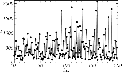
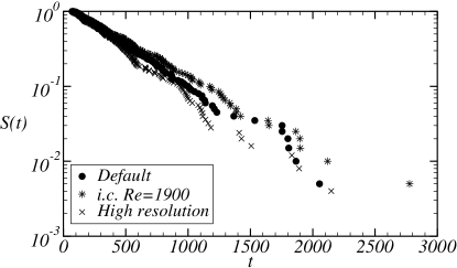
Figure 2: $(a)$ Relaminarisation times for reduction simulations from $\mbox{{Re}}=2000$ to $\mbox{{Re}}=1860$ as a function of initial condition. $(b)$ Survivor function at $\mbox{{Re}}=1860$ from the data in $(a)$ (circles), initial conditions at $\mbox{{Re}}=1900$ (stars) and high numerical resolution (crosses).

Figure 2$(a)$ shows relaminarisation times following a reduction of the Reynolds number to $\mbox{{Re}}=1860$ as a function of initial condition. The times from here onwards are shown in $D/U$ units. The large fluctuations in the data indicate that consecutive initial conditions result in uncorrelated lifetimes. From these data, the corresponding survivor function $S(t)$ has been obtained and is plotted as circles in the logarithmic scale of figure 2$(b)$. The approximately constant slope of $S(t)$ implies the memoryless nature of the relaminarisation process. To verify the numerical resolution, the number of modes in the azimuthal and axial directions was increased by $33\%$ and the number of finite-difference points by $25\%$. The number of degrees of freedom is greater than $2.2$ times that of the default resolution. The results are plotted in figure 2$(b)$ as crosses and are within statistical certainty of the default prediction (see inset of figure 5). Thus, we conclude that the turbulent puffs are accurately resolved.

The impact of the mechanism to initiate the turbulent state on the relaminarisation probabilities has been object of much debate in the literature (Willis & Kerswell, 2007; Schneider & Eckhardt, 2008; de Lozar & Hof, 2009). Indeed, the reduction procedure of Peixinho & Mullin (2006) was introduced as an attempt to minimise the effect of initial conditions in lifetime measurements. Robustness of the survivor function has been examined here by repeating the lifetime simulations at $\mbox{{Re}}=1860$ but using three additional sets of initial conditions, each of them consisting of $200$ velocity field snapshots. First, initial conditions of a puff simulation at $\mbox{{Re}}=2200$ were used, representing a much greater initial change of the Re over the default reduction from $\mbox{{Re}}=2000$. This was again repeated but from a puff simulation at $\mbox{{Re}}=1925$. Finally, following Willis & Kerswell (2007) randomly selected velocity snapshots of several puffs at $\mbox{{Re}}=1900$ were used. The stars in figure 2$(b)$ show the results of the reduction from $\mbox{{Re}}=1900$, whereas results from $\mbox{{Re}}=2200$ and $1925$ are not shown to avoid crowding the figure. All three additional cases render characteristic lifetimes within the $95\%$ confidence interval about the default prediction (see inset of figure 5), higlighting the independence of the lifetime statistics from initial conditions. These results confirm the experimental findings of de Lozar & Hof (2009), who have demonstrated the invariance of the lifetime distributions by using four different experimental protocols to generate the turbulent puffs.

4 Statistical analysis of turbulent lifetimes

An exponential distribution of turbulent lifetimes is one of the main pillars of the strange saddle paradigm for the transition to turbulence in shear flows (Eckhardt, 2008). In practice, the distributions are exponential only for $t>t_{0}>0$, where $t_{0}$ depends on the procedure to initiate turbulence and Reynolds number in a non-trivial manner (Schneider & Eckhardt, 2008; de Lozar & Hof, 2009). When Re is suddenly quenched in the reduction experiments, the puff is forced to quickly readjust to the new flow rate and this could cause immediate relaminarisation. In phase space, this is equivalent to a trajectory not having approached the strange saddle. Thus, consistently determining $t_{0}$ constitutes a challenge in lifetime studies of shear flows. The problem stems from the difficulties in discriminating between a trajectory that has shown very short turbulent behavior and one that has directly relaminarised. This is especially delicate in the low Re regime, where a large part of the sample features lifetimes shorter than $t_{0}$.

The hazard function of a lifetime distribution, defined as

$$h(t)=-\dfrac{d}{dt}\log(S(t)),$$ (4)

specifies the instantaneous rate of death at time $t$, i.e. $h(t)\delta t$ is the approximate probability of death in $[t,t+\delta t]$ given survival up to time $t$. For an exponential distribution, the hazard function is constant $h(t)=1/\tau$, where $\tau=\langle t\rangle$ is the mean lifetime of the population. This corresponds to a memoryless process. In the theory of dynamical systems, the escape rate from the saddle is defined as $\kappa=1/\tau$ (Tél & Lai, 2008).

4.1 Determining $t_{0}$: onset of the strange saddle

$(a)$	$(b)$

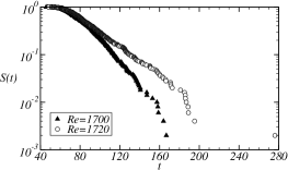
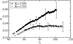
Figure 3: $(a)$ Survivor function of turbulent lifetimes at $\mbox{{Re}}=1720$ (circles) and $1700$ (triangles) obtained with $500$ simulations each. $(b)$ Escape rates $\kappa=1/\tau$ as a function of $t_{0}$. The error bars correspond to $95\%$ confidence intervals around the $\kappa$ predictions.

Figure 3$(a)$ is a logarithmic plot of the lifetime distribution at $\mbox{{Re}}=1700$ (triangles) and $\mbox{{Re}}=1720$ (circles). Their corresponding escape rates have been computed by subsequently excluding from the sample puffs that have decayed before a given time $t_{0}$, i.e. $\kappa(t_{0})=1/\tau(t_{0})$ with $\tau(t_{0})=\langle t-t_{0}|t>t_{0}\rangle$. Figure 3$(b)$ shows the resulting values of $\kappa(t_{0})$ as a function of cutoff time $t_{0}$. Note that as $t_{0}$ is increased, the size of the sample used to estimate $\kappa$ is progressively reduced from $500$ to $100$, resulting in greater error bars. For $\mbox{{Re}}=1720$, the plot approaches a horizontal line at about $t_{0}\simeq 72$, indicating a constant hazard function and thus exponentially distributed lifetimes. Hence, we conclude that at $\mbox{{Re}}=1720$ the escape rate of turbulent trajectories from the saddle is $\kappa\simeq 0.035$, whereas trajectories that have decayed before $t_{0}\simeq 72$ cannot be counted as having visited the saddle. Overall $t_{0}$ increases slightly from $72$ at $\mbox{{Re}}=1720$ to $95$ at $\mbox{{Re}}=1820$. Meanwhile, the number of trajectories decaying without visiting the saddle decreases as Re increases, and at $\mbox{{Re}}=1860$ almost all trajectories are attracted to the saddle.

No evidence of exponential behaviour in the lifetimes for $\mbox{{Re}}<1720$ has been found. This is illustrated by the hazard function at $\mbox{{Re}}=1700$, plotted as triangles in figure 3$(b)$. Despite the initial similarity with $\mbox{{Re}}=1720$, the escape rate for $\mbox{{Re}}=1700$ does not settle to a constant value but increases monotonously. This implies that the probabilities of relaminarisation depend on the history of the turbulent trajectory. Similar results have been found for $\mbox{{Re}}=1580$ and $1640$ using $500$ simulations in each case. Hence, the data at low $\mbox{{Re}}<1720$ cannot be used to extrapolate lifetime scaling with Re, at least not under the assumption of a memoryless process corresponding to the escape from a strange saddle.

4.2 Estimation of characteristic turbulent lifetimes

Characteristic turbulent lifetimes are estimated from an exponential distribution,

$$S(t)=\exp[(t-t_{0})/\tau_{\text{true}}],$$ (5)

with the sample mean, which is the the Maximum Likelihood Estimator (MLE) of the parameter $\tau_{\text{true}}$. However, the observation time-span is finite in practice, which implies that the data need to be truncated and therefore the sample mean cannot be obtained. A lifetime sample of size $n$ with truncation after $r$ decays is known as censored data of Type-II (Lawless, 2003). In this case, the MLE of $\tau_{\text{true}}$ is given by

$$\tau=\dfrac{1}{r}\Big{[}\sum_{i=1}^{r}t_{i}+(n-r)t_{r}\Big{]},$$ (6)

where $t_{0}+t_{i}$ is the lifetime of the $i$th puff to decay, hence $t^{*}=t_{0}+t_{r}$ being the time where the simulations were truncated. The corresponding exact confidence intervals, at level $1-\alpha$, are

$$\tau_{\text{true}}\,\in\,\tau\times\big{[}2r/\chi^{2}_{2r,1-\alpha/2},2r/\chi^{2}_{2r,\alpha/2}\big{]},$$ (7)

where $\chi^{2}_{m,p}$ is the $p$th quantile of the chi-squared distribution with $m$ degrees of freedom. It is worth noting that for uncensored data ($r=n$), the sample mean is recovered as MLE, and more importantly, that the relative size of the confidence intervals is uniquely determined by the number of runs $r$ that have decayed. In the uncensored case the Central Limit Theorem yields approximate $95\%$ confidence intervals $\tau\times(1\pm 1.96/\sqrt{n})$, and the need for a large number of observations is a consequence of the slow convergence with $n$.

$(a)$	$(b)$

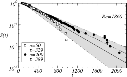
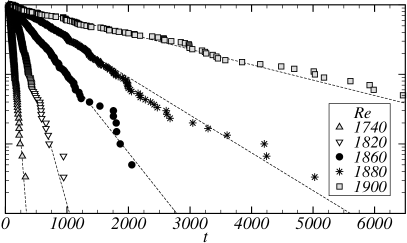
Figure 4: $(a)$ Survivor function at $\mbox{{Re}}=1860$ obtained from sample sizes $n=50$ (squares) and $200$ (circles). The solid (dashed) line is the curve $\exp[(t-t_{0})/\tau]$ for $n=50$ ($200$), where $\tau$ has been estimated from (6). The shaded area between the two dotted lines corresponds to the confidence interval (7) for $n=50$. $(b)$ Survivor function of turbulent lifetimes at several Reynolds numbers. For clarity, only part of the Re investigated are shown.

Figure 4$(a)$ shows the survivor function at $\mbox{{Re}}=1860$ for the first $50$ runs in figure 2$(a)$ and for the full sample $n=200$. The mean lifetimes have been estimated from (6) and are plotted as solid and dash lines illustrating the curves $\exp[(t-t_{0})/\tau]$. Although the characteristic lifetime from the sub-sample $n=50$ is shorter, its $95\%$ confidence interval (7), spanned by the shaded area in the figure, includes the result from the full sample.

5 Lifetime scaling with Re: the transient nature of puff turbulence

In order to shed light on the discrepancies in scaling of turbulent lifetimes present in the literature, we have extended the Reynolds number range in the numerical simulations up to $\mbox{{Re}}=1900$. The results are presented in figure 4$(b)$, showing survivor functions at several Re in a logarithmic scale. The sample sizes have been subsequently increased until each data-set unambiguously showed the exponential distribution. In particular, between $200$ and $500$ simulations were run for $\mbox{{Re}}\in[1720,1880]$, whereas at $Re=1900$ only $100$ cases were simulated due to the computational costs incurred in very long time integrations. In addition, the simulations at $Re=1900$ were stopped when $96$ puffs had decayed, leaving only $4$ survivors at $t^{*}\simeq 6500$.

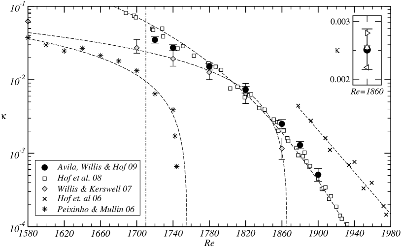
Figure 5: Escape rate $\kappa$ scaling with Re as obtained from the mean lifetimes of the survivor functions in figure 4 (shown in black circles). The vertical line marks the approximate onset of the strange saddle. The inset shows the escape rate at $\mbox{{Re}}=1860$: default reduction from $\mbox{{Re}}=2000$ (black circle and $95\%$ confidence interval), reductions from $\mbox{{Re}}=2200,1925,1900$ ($\triangle$,$\triangledown$,$\triangleleft$) and high numerical resolution ($\triangleright$).

From the survivor functions in figure 4$(b)$ escape rates $\kappa=1/\tau$ have been estimated using (6) and are shown as black circles in the logarithmic scale of figure 5. Confidence intervals at the $95\%$ level, obtained from (7), have been plotted and may be regarded as error bars due to sample size. The results of the high resolution runs and reductions from $\mbox{{Re}}=2200$, $1925$ and $1900$ to $\mbox{{Re}}=1860$ fall within the $95\%$ confidence interval of the default case and are only shown in the inset to avoid overlapping the figure. Overall, the results are in excellent quantitative agreement with the experimental relaminarisation probabilities of Hof et al. (2008), shown as squares. With increasing Re, $\kappa$ decreases extremely fast, corresponding to a super-exponential increase in turbulent lifetimes. It is worth noting that the measurements of Hof et al. (2008) extend up to $\mbox{{Re}}=2050$, with their super-exponential fit providing a very good approximation over the full data set.

The agreement with the simulations of Willis & Kerswell (2007) is very good for $\mbox{{Re}}=1740,1780,1820$. For $\mbox{{Re}}\lesssim 1720$ we have shown that the lifetimes are not exponentially distributed (vertical line). The discrepancy of the point at $\mbox{{Re}}=1860$ is attributed mainly to statistical uncertainty. There $\tau_{\text{true}}$ was estimated with $40$ simulations, of which only $28$ had decayed when truncated at $t^{*}\simeq 1000$. The upper end of their confidence interval is close to the experimental value of Hof et al. (2008) and the present computations, although there is still a small difference. We remark, for example, that had the $40$ initial conditions $i\in[90,130]$ of figure 2$(a)$ been used here to estimate $\tau_{\text{true}}$, the result would be compatible with the estimate provided by Willis & Kerswell (2007). The escape rates and confidence intervals shown in figure 5 are those given in their re-analysis (Willis & Kerswell, 2008), using bootstrapping. Using the method in §4.2 on their original data shifts the point at $\mbox{{Re}}=1860$ by only $10\%$ in the direction of the current data set, with a $10\%$ larger confidence interval than that shown.

The experiments of Hof et al. (2006) appear to be shifted by $2.5\%$ in Re with respect to the numerical simulations and later experiments of Hof et al. (2008). Their exponential fit, however, provides a good approximation of the slope of $\kappa$ over $2$ orders of magnitude. Similarly, applying a $7\%$ shift in Re, the data of Peixinho & Mullin (2006) overlaps for most of the range. Significant differences between their results and the results presented here, then remain only for their two highest Re. A procedural difference is the manner in which the puffs were generated. It has been shown here and by de Lozar & Hof (2009), however, that the initial condition has no influence other than on $t_{0}$. A more likely source of difference is the difficulty of inferring the lifetime from the data. At high Re, a short pipe implies very few relaminarisations and therefore a very large range of possible $\tau$ according to (6). For example, at $\mbox{{Re}}=1745$ Peixinho & Mullin (2006) obtained a mean lifetime of $\tau=1515$. For an observation distance of $500D$ after reducing Re, this corresponds to $r\leq 3$ decays out of $n=50$ experimental runs, yielding a confidence interval $\tau_{\text{true}}\times[629,7346]$. Nevertheless, we must acknowledge that Peixinho & Mullin (2006) were first to experimentally demonstrate the very rapid increase in lifetimes over a small range of Reynolds numbers.

6 Conclusions

The transition to turbulence in pipe flow has been recently linked to the presence of a strange saddle in the phase space of the Navier–Stokes equations (see e.g.  Eckhardt, 2008). One of the predictions of this emerging paradigm is that the turbulent lifetimes, the time prior to escaping the saddle, should be exponentially distributed. We have shown that the distributions are indeed exponential by substantially increasing the sample size and thus reducing statistical uncertainty with respect to previous works. In order to recover the true escape rate, a substantially larger sample size than previously used is necessary.

We have demonstrated that initial conditions from puffs at $\mbox{{Re}}=2200,2000,1925,1900$ render the same characteristic lifetimes after reduction to $\mbox{{Re}}=1860$, which verifies that the same turbulent state is visited. Here, contrary to the possibility that the turbulent state be difficult to reach when changing the Reynolds number, the number of trajectories which fail to approach the saddle is actually low (small $t_{0}$). This reflects structural similarity of the initial condition with the state at the final Re.

Interestingly, the onset of the exponential distributions is rather sharp in Re at about $\mbox{{Re}}\lesssim 1720$. This suggests a bifurcation event that gives rise to the strange saddle. The onset of meta-stable transients has been characterized in plane Couette flow experiments by Bottin & Chaté (1998) and Bottin et al. (1998), who measured the average turbulent fraction. The change in distributional shape revealed here provides an alternative reliable means of quantifying a lower bound for meta-stable turbulence, and is appropriate when considering single isolated disturbances.

Our results support the view of localised turbulence as a strange repellor, with lifetimes increasing super-exponentially with Re as in the experiments of Hof et al. (2008). A similar scaling has been recently reported by Borrero-Echeverry, Tagg & Schatz (2009) in Taylor–Couette flow with stationary inner cylinder and previously by Schoepe (2004) in super-fluid turbulence. To our knowledge the quantitative agreement of the presented numerical simulations with experiment is unprecedented in transition studies. It validates the use of periodic boundary conditions and testifies the high demands on numerical resolution and domain sizes which are required to faithfully capture the relevant dynamics of turbulence.