Stability of Lagrange elements for the mixed Laplacian

Abstract.

The stability properties of simple element choices for the mixed formulation of the Laplacian are investigated numerically. The element choices studied use vector Lagrange elements, i.e., the space of continuous piecewise polynomial vector fields of degree at most $r$, for the vector variable, and the divergence of this space, which consists of discontinuous piecewise polynomials of one degree lower, for the scalar variable. For polynomial degrees $r$ equal 2 or 3, this pair of spaces was found to be stable for all mesh families tested. In particular, it is stable on diagonal mesh families, in contrast to its behaviour for the Stokes equations. For degree $r$ equal 1, stability holds for some meshes, but not for others. Additionally, convergence was observed precisely for the methods that were observed to be stable. However, it seems that optimal order $L^{2}$ estimates for the vector variable, known to hold for $r>3$, do not hold for lower degrees.

1. Introduction

In this note, we consider approximations of the mixed Laplace equations with Dirichlet boundary conditions: Given a source $g$, find the velocity $u$ and the pressure $p$ such that

$$u-\operatorname{grad}p=0,\;\operatorname{div}u=g\;\text{ in }\Omega,\quad\quad p=0\;\text{ on }\partial\Omega,$$

for a domain $\Omega\subset\mathbb{R}^{2}$ with boundary $\partial\Omega$. The equations offer the classical weak formulation: Find a square integrable vector field with square integrable divergence $u\in H(\operatorname{div},\Omega)$ and a square integrable function $p\in L^{2}(\Omega)$ such that

(1.1) $$\int_{\Omega}u\cdot v+q\,\operatorname{div}u+p\,\operatorname{div}v=\int_{\Omega}g\,q$$

for all $v\in H(\operatorname{div},\Omega)$ and $q\in L^{2}(\Omega)$. The above formulation can be discretized using a pair of finite dimensional spaces $V_{h}\subset H(\operatorname{div},\Omega)$, $Q_{h}\subset L^{2}(\Omega)$, yielding discrete approximations $u_{h}\in V_{h}$ and $p_{h}\in Q_{h}$ satisfying (1.1) for all $v\in V_{h}$ and $q\in Q_{h}$.

As is well-known, the spaces $V_{h}$ and $Q_{h}$ must satisfy certain stability, or compatibility, conditions for the discretization to be well-behaved [7]. More precisely, there must exist positive constants $\alpha$ and $\beta$ such that for any $h$,

(1.2a) $$0<\alpha\leq\alpha_{h}=\inf_{u\in\mathcal{Z}_{h}}\sup_{v\in\mathcal{Z}_{h}}\frac{\langle u,v\rangle}{\|u\|_{\operatorname{div}}\|v\|_{\operatorname{div}}},$$

(1.2b) $$0<\beta<\beta_{h}^{\operatorname{div}}=\inf_{q\in Q_{h}}\sup_{v\in V_{h}}\frac{\langle\operatorname{div}v,q\rangle}{\|v\|_{\operatorname{div}}\|q\|_{0}}.$$

Here, $\|\cdot\|_{\operatorname{div}}$ and $\|\cdot\|_{0}$ denote the norms on $H(\operatorname{div},\Omega)$ and $L^{2}(\Omega)$, $\langle\,\cdot\,,\,\cdot\,\rangle$ is the $L^{2}(\Omega)$ inner product and

(1.3) $$\mathcal{Z}_{h}=\{v\in V_{h}\,|\;\langle\operatorname{div}v,q\rangle=0\quad\forall\,q\in Q_{h}\}.$$

The two conditions will be referred to as the Brezzi coercivity and the Brezzi inf-sup condition for the mixed Laplacian. The classical conforming discretizations of (1.1) rely on the finite element families of Raviart and Thomas [18] or Brezzi, Douglas and Marini [8] for the space $V_{h}\subset H(\operatorname{div})$ in order to satisfy these conditions.

In this note, we shall consider the Lagrange vector element spaces, that is, continuous piecewise polynomial vector fields defined relative to a triangulation $\mathcal{T}_{h}$, for the space $V_{h}$. This is motivated by the following reasons. First, these spaces are fairly inexpensive, simple to implement and post-process and in frequent use for other purposes. Second, such pairs would allow continuous approximations of the velocity variable, or when viewed in connection with linear elasticity, lay the ground for continuous approximations of the stress tensor. Moreover, in the recent years, there has been an interest in mixed finite element discretizations that are both stable for (1.1) and for the Stokes equations:

(1.4) $$\int_{\Omega}\operatorname{grad}u:\operatorname{grad}v+q\,\operatorname{div}u+p\,\operatorname{div}v=\int_{\Omega}f\,v$$

for all $v\in H^{1}(\Omega;\mathbb{V})$ such that $\int_{\Omega}v=0$ and all $q\in L^{2}(\Omega)$. The search for conforming such discretizations is complicated by the fact that the existing, stable discretizations of (1.1) are such that $V_{h}\not\subset H^{1}(\Omega;\mathbb{V})$. On the other hand, the existing stable discretizations of (1.4) are typically unstable for (1.1) [14]. The existence of stable discretizations $V_{h}\times Q_{h}$ of (1.1) such that $V_{h}\subset H^{1}(\Omega;\mathbb{V})$ becomes a natural separate question. Unfortunately, there are no known such finite element discretizations that are stable for any admissible triangulation family $\{\mathcal{T}_{h}\}$. In this note, we aim to numerically examine cases where a reduced stability property may be identified. In this sense, the investigations here are in the spirit of the work of Chapelle and Bathe [10] and Qin [17].

For a family of conforming discretizations $\{V_{h}\times Q_{h}\}_{h}$ of (1.1) such that $\operatorname{div}V_{h}\subseteq Q_{h}$ for each $h$, the condition (1.2a) is trivial. The stability conditions thus reduce to the condition (1.2b), namely the question of bounded Brezzi inf-sup constant $\beta_{h}^{\operatorname{div}}$. On the other hand, recall that for the Stokes formulation (1.4), the corresponding Brezzi coercivity condition is trivial by the Poincaré inequality. Hence, for any family of conforming discretizations, the stability conditions for Stokes reduce to that of a uniform bound for the Brezzi inf-sup constant $\beta_{h}^{1}$. Here,

(1.5) $$\beta_{h}^{1}=\inf_{q\in Q_{h}}\sup_{v\in V_{h}}\frac{\langle\operatorname{div}v,q\rangle}{\|v\|_{1}\|q\|_{0}}.$$

when $V_{h}\subset H^{1}(\Omega;\mathbb{V})$, $Q_{h}\subset L^{2}(\Omega)$ and $\|\cdot\|_{1}$ denotes the norm on $H^{1}(\Omega)$. Further, such a bound immediately gives (1.2b) since $\beta_{h}^{1}\leq\beta_{h}^{\operatorname{div}}$ by definition. Hence, if $\operatorname{div}V_{h}\subseteq Q_{h}$, stability for Stokes immediately gives stability for the mixed Laplacian.

The conditions $\operatorname{div}V_{h}\subseteq Q_{h}$ and $V_{h}\subset H^{1}(\Omega;\mathbb{V})$ are clearly satisfied by the element pairs consisting of continuous piecewise polynomial vector fields of degree less than or equal to $r$ and discontinuous piecewise polynomials of degree $r-1$, for $r=1,2,\dots$. This family could be viewed as an attractive family of elements for both the Stokes equations and the mixed Laplacian. However, the Brezzi inf-sup constant(s) will not be bounded for all $r$. For $r\geq 4$, Scott and Vogelius demonstrated that these finite element spaces will be stable for the Stokes equations on triangulations that have no nearly singular vertices, that is, triangulations that are not singular in the appropriate sense [19]. The lower order cases, $1\leq r\leq 3$, were studied carefully by Qin, concluding that the elements are not stable in general [17]. However, they are stable for some specific families of triangulations, and can be stabilized by removal of spurious pressure modes on some other classes of triangulations. (The space $\mathcal{N}_{h}$ of spurious pressure modes is defined in (2.10) below.) In general, the stability of finite element spaces for the Stokes equations has been extensively investigated. In addition to the previous references, surveys are presented in [3, 9]. However, to our knowledge, a careful study of the lower order cases has not been conducted for the mixed Laplacian.

As the stability for the mixed Laplacian is a weaker requirement when $\operatorname{div}V_{h}\subseteq Q_{h}$, there may be a greater class of triangulations for which the elements form a stable discretization. In fact, this is known to be true. One example is provided by the pairing of continuous piecewise linear vector fields $V_{h}$ and the subspace of discontinuous piecewise constants $Q_{h}$ such that $Q_{h}=\operatorname{div}V_{h}$ on crisscross triangulations of the unit square. Qin proved that there does not exist a $\beta>0$ such that $\beta_{h}^{1}>\beta$ for any $h$ [17, Lemma 7.3.2]. On the other hand, Boffi et al. proved that such a bound does exists for $\beta_{h}^{\operatorname{div}}$ [4]. We shall present numerical evidence suggesting that there is a range of triangulations for which this phenomenon occurs. The main results are summarized below.

Spurious modes:

For $r=2,3$ and for all triangulations tested, the dimension of the space $\mathcal{N}_{h}$ of spurious modes is equal to the number of interior singular vertices $\sigma$. However, for $r=1$ and one of the triangulation families studied (“Flipped”, which is defined in Figure 1), $\dim\mathcal{N}_{h}$ is strictly greater than $\sigma$.

Stability:

For all triangulations we have tested, the method seems at least reduced stable (i.e., stable after removal of spurious modes, if any), for $r=2,3$. This is in contrast to the situation for the Stokes equations, where for some triangulations, such as the diagonal triangulation, the method is not reduced stable for $r=2,3$, while for other triangulations, it is. For $r=1$, reduced stability holds for some triangulations, but fails for others, including the diagonal triangulation.

Convergence:

We also studied convergence of the method on diagonal triangulations. For such meshes, the method was observed to be stable for $r>1$, but unstable for $r=1$. Theory predicts optimal convergence of $p$ in $L^{2}(\Omega)$ and $u$ in $H(\operatorname{div},\Omega)$ for a stable method and this is in fact what was observed. Such optimal convergence holds for $r=2,3,4$, but not in the apparently unstable case $r=1$. In the case $r\geq 4$, it is known that $u$ converges at one order higher in $L^{2}(\Omega)$ than in $H(\operatorname{div},\Omega)$. No such increase of order was observed for $r<4$.

The note is organized as follows. We introduce further notation and summarize some key points of the theory of mixed finite element methods in Section 2. Further, we derive some eigenvalue problems associated with the stability conditions and give a characterization of the Brezzi inf-sup constant for the mixed Laplacian $\beta_{h}^{\operatorname{div}}$ in Section 3. These eigenvalue problems applied to the Stokes equations were also stated by Malkus [13] and (in part) by Qin [17] and provide a foundation for numerical investigations of the Brezzi stability conditions. Based on these general results, Section 4 is devoted to the study of continuous piecewise polynomials in two dimensions for the velocity and discontinuous piecewise polynomials for the pressure.

2. Notation and preliminaries

The notion of reduced stability of families of mixed finite element spaces is a key point in this note. In order to make this notion precise, this preliminary section aims to introduce notation and summarize the stability notions for finite element discretizations of abstract saddle point problems.

If $V$ is an inner product space, we denote the dual space by $V^{*}$, the inner product on $V$ by $\langle\,\cdot\,,\,\cdot\,\rangle_{V}$ and the induced norm by $\|\cdot\|_{V}$. Let $\Omega$ be an open and bounded domain in $\mathbb{R}^{d}$ with boundary $\partial\Omega$. We let $H^{m}(\Omega)$, for $m=0,1,\dots$, denote the standard Sobolev spaces of square integrable functions with $m$ weak derivatives and denote their norm by $\|\cdot\|_{m}$. Accordingly, $H^{0}(\Omega)=L^{2}(\Omega)$. The space of polynomials of degree $r$ on $\Omega$ is denoted $\mathcal{P}_{r}(\Omega)$. The space of vectors in $\mathbb{R}^{d}$ is denoted $\mathbb{V}$ and in general, $X(\Omega;\mathbb{V})$ denotes the space of vector fields on $\Omega$ for which each component is in $X(\Omega)$. For brevity however, the space of vector fields in $L^{2}(\Omega;\mathbb{V})$ with square integrable divergence is written $H(\operatorname{div},\Omega)$ with norm $\|\cdot\|_{\operatorname{div}}$ and semi-norm $|\cdot|_{\operatorname{div}}=\|\operatorname{div}\cdot\,\|_{0}$. The subscripts and the reference to the domain $\Omega$ will be omitted when considered superfluous.

Let $\mathcal{T}_{h}$ denote an admissible simplicial tessellation of $\Omega$, $h$ measuring the mesh size of the tessellation. We shall frequently refer to spaces of piecewise polynomials defined relative to such, and label the spaces of continuous, and discontinuous, piecewise polynomials of degree less than or equal to $r$ as follows.

$$\mathcal{P}^{c}_{r}=\mathcal{P}^{c}_{r}(\mathcal{T}_{h}) =\{p\in H^{1}(\Omega)\,|\;p|_{K}\in\mathcal{P}_{r}(K)\quad\forall\,K\in\mathcal{T}_{h}\}\quad r=1,2,\dots,$$

$$\mathcal{P}_{r}=\mathcal{P}_{r}(\mathcal{T}_{h}) =\{p\in L^{2}(\Omega)\,|\;p|_{K}\in\mathcal{P}_{r}(K)\quad\forall\,K\in\mathcal{T}_{h}\}\quad r=0,1,\dots.$$

The classical abstract saddle point problem reads as follows [7, 9]: for given Hilbert spaces $V$ and $Q$ and data $(f,g)\in V^{*}\times Q^{*}$, find $(u,p)\in V\times Q$ satisfying

(2.1) $$a(u,v)+b(v,p)+b(u,q)=\langle f,v\rangle+\langle g,q\rangle\quad\forall\,(v,q)\in V\times Q,$$

where $a$ and $b$ are assumed to be continuous, bilinear forms on $V\times V$ and $V\times Q$, respectively. We shall assume here and throughout that $a$ is symmetric. Following [2], there exists a unique solution $(u,p)$ of (2.1), if and only if the continuous Babuška inf-sup constant

(2.2) $$\gamma=\inf_{0\not=(u,p)}\sup_{0\not=(v,q)}\frac{a(u,v)+b(v,p)+b(u,q)}{\|(u,p)\|_{V\times Q}\|(v,q)\|_{V\times Q}}$$

is positive. By [7], this holds if and only if the continuous Brezzi coercivity and Brezzi inf-sup constants are positive. These are defined as

(2.3) $$\alpha=\inf_{0\not=u\in\mathcal{Z}}\sup_{0\not=v\in\mathcal{Z}}\frac{a(u,v)}{\|u\|_{V}\|v\|_{V}},$$

(2.4) $$\beta=\inf_{0\not=q\in Q}\sup_{0\not=v\in V}\frac{b(v,q)}{\|v\|_{V}\|q\|_{Q}},$$

respectively, where $\mathcal{Z}=\{v\in V\,|\;b(v,q)=0\quad\forall\,q\in Q\}$.

Given finite dimensional spaces $V_{h}\subset V$ and $Q_{h}\subset Q$, defined relative to a tessellation $\mathcal{T}_{h}$ of $\Omega$, the Galerkin discretization of (2.1) takes the form: Find $(u_{h},p_{h})\in V_{h}\times Q_{h}$ satisfying

(2.5) $$a(u_{h},v)+b(v,p_{h})+b(u_{h},q)=\langle f,v\rangle+\langle g,q\rangle\quad\forall\,(v,q)\in V_{h}\times Q_{h}.$$

On the discrete level, the Babuška inf-sup, Brezzi coercivity and Brezzi inf-sup constants are defined as

(2.6) $$\gamma_{h} :=\inf_{0\not=(u,p)\in V_{h}\times Q_{h}}\sup_{0\not=(v,q)\in V_{h}\times Q_{h}}\frac{a(u,v)+b(v,p)+b(u,q)}{\|(u,p)\|_{V\times Q}\|(v,q)\|_{V\times Q}},$$

(2.7) $$\alpha_{h} :=\inf_{0\not=u\in\mathcal{Z}_{h}}\sup_{0\not=v\in\mathcal{Z}_{h}}\frac{a(u,v)}{\|u\|_{V}\|v\|_{V}},$$

(2.8) $$\beta_{h} :=\inf_{0\not=q\in Q_{h}}\sup_{0\not=v\in V_{h}}\frac{b(v,q)}{\|v\|_{V}\|q\|_{Q}},$$

where

(2.9) $$\mathcal{Z}_{h}=\{v\in V_{h}\,|\;b(v,q)=0\quad\forall\,q\in Q_{h}\}.$$

For given $V_{h}\times Q_{h}$, there exists a unique solution of (2.5) if and only if $\alpha_{h}$ and $\beta_{h}$ (or equivalently $\gamma_{h}$) are positive. Furthermore, for a family of discretization spaces $V_{h}\times Q_{h}$ parameterized by $h$, if $\alpha_{h}$ and $\beta_{h}$ are uniformly bounded from below, then one obtains the quasi-optimal approximation estimate [7]:

$$\|u-u_{h}\|_{V}+\|p-p_{h}\|_{Q}\leq C\left(\inf_{v\in V_{h}}\|u-v\|_{V}+\inf_{q\in Q_{h}}\|p-q\|_{Q}\right),$$

with $C$ depending only on the bounds for $\alpha_{h}$ and $\beta_{h}$ and bounds on the bilinear forms $a$ and $b$. The uniform boundedness condition motivates the notion of stability for pairs of finite element spaces.

Definition 2.1 (Stable discretization).

A family of finite element discretizations $\{V_{h}\times Q_{h}\}_{h}$ is stable in $V\times Q$ if the Brezzi coercivity and inf-sup constants $\alpha_{h}$ and $\beta_{h}$ (or equivalently the Babuška inf-sup constant $\gamma_{h}$) are bounded from below by a positive constant independent of $h$.

In accordance with standard terminology, we say that $\{V_{h}\times Q_{h}\}_{h}$ satisfies the Brezzi coercivity or inf-sup conditions if $\alpha_{h}$ or $\beta_{h}$, respectively, are uniformly bounded from below.

There are families of discretizations that are not stable in the sense defined above, but have a reduced stability property. More precisely, for a pair $V_{h}\times Q_{h}$ consider the space of spurious modes $\mathcal{N}_{h}\subseteq Q_{h}$:

(2.10) $$\mathcal{N}_{h}=\{q\in Q_{h}\,|\;b(v,q)=0\quad\forall\,v\in V_{h}\}.$$

For a stable discretization, $\mathcal{N}_{h}$ contains only the zero element. Indeed, $\beta_{h}=0$ if and only if $\mathcal{N}_{h}$ contains non-zero elements. If $\mathcal{N}_{h}$ is non-trivial, it is natural to consider the reduced space $\mathcal{N}_{h}^{\perp}$, the orthogonal complement of $\mathcal{N}_{h}$ in $Q_{h}$, in place of $Q_{h}$. This motivates the definition of the reduced Brezzi inf-sup constant, relating to the stability of $V_{h}\times\mathcal{N}_{h}^{\perp}$:

(2.11) $$\tilde{\beta}_{h}=\inf_{0\not=q\in\mathcal{N}_{h}^{\perp}}\sup_{0\not=v\in V_{h}}\frac{b(v,q)}{\|v\|_{V}\|q\|_{Q}},$$

and the following definition of reduced stable. By definition, $\tilde{\beta}_{h}\not=0$.

Definition 2.2 (Reduced stable discretization).

A family of discretizations $\{V_{h}\times Q_{h}\}_{h}$ is reduced stable in $V\times Q$ if the Brezzi coercivity constant $\alpha_{h}$ and the reduced Brezzi inf-sup constant $\tilde{\beta}_{h}$, defined by (2.7) and (2.11), are bounded from below by a positive constant independent of $h$.

3. Eigenvalue problems related to the Babuška-Brezzi constants

For a given set of discrete spaces, the Babuška and Brezzi constants defined by (2.6)–(2.8) can be computed by means of eigenvalue problems. The form and properties of the eigenvalue problem associated with the Brezzi inf-sup constant for the Stokes equations were discussed by Qin in [17]. Since also the Brezzi coercivity constant plays a role for the mixed Laplacian, we begin this section by deriving how the Brezzi coercivity constant can be computed by similar eigenvalue problems. Actually, in our application in Section 4, the Brezzi coercivity condition will be automatic, however, we discuss it here in the abstract case, for the sake of completeness. These eigenvalue problems were also stated, and carefully analysed from an algebraic view-point, by Malkus [13] in connection with the displacement-pressure formulation of the linear elasticity equations. We continue by observing that the continuous Brezzi inf-sup constant can be naturally associated with the smallest eigenvalue of the Laplacian itself.

3.1. Eigenvalue problems for the discrete Babuška-Brezzi constants

Let $V_{h}\subset V$ and $Q_{h}\subset Q$ be given finite dimensional spaces as before. It follows easily from the definition that the Babuška inf-sup constant $\gamma_{h}=|\lambda_{\min}|$ when $\lambda_{\min}$ is the smallest (in modulus) eigenvalue of the following generalized eigenvalue problem: Find $\lambda\in\mathbb{R}$, $0\not=(u,p)\in V_{h}\times Q_{h}$ satisfying

(3.1) $$a(u,v)+b(v,p)+b(u,q)=\lambda\left(\langle u,v\rangle_{V}+\langle p,q\rangle_{Q}\right)\quad\forall\,(v,q)\in V_{h}\times Q_{h}.$$

The following lemma identifies an eigenvalue problem associated with the Brezzi inf-sup constant.

Lemma 3.1 (Qin [17, Lemma 5.1.1 – 5.1.2]).

Let $\lambda_{\min}$ be the smallest eigenvalue of the following generalized eigenvalue problem: Find $\lambda\in\mathbb{R}$, $0\not=(u,p)\in V_{h}\times Q_{h}$ satisfying

(3.2) $$\langle u,v\rangle_{V}+b(v,p)+b(u,q)=-\lambda\langle p,q\rangle_{Q},\quad\forall\,(v,q)\in V_{h}\times Q_{h}.$$

Then, $\lambda\geq 0$ and for $\beta_{h}$ defined by (2.8), $\beta_{h}=\sqrt{\lambda_{\min}}$.

It can also be shown that the reduced Brezzi inf-sup constant $\tilde{\beta}_{h}$ equals the square-root of the smallest non-zero eigenvalue of (3.2) [17, Theorem 5.1.1].

The Babuška and Brezzi inf-sup constants are thus easily computed, given bases for the spaces $V_{h}$ and $Q_{h}$. As for (3.1), it is easily seen that the Brezzi coercivity constant $\alpha_{h}=|\lambda_{\min}|$ where $\lambda_{\min}$ is the smallest (in modulus) eigenvalue of the eigenvalue problem: Find $\lambda\in\mathbb{R}$ and $0\not=u\in\mathcal{Z}_{h}$ such that

(3.3) $$a(u,v)=\lambda\langle u,v\rangle_{V}\quad\forall\;v\in\mathcal{Z}_{h}.$$

However, a basis for $\mathcal{Z}_{h}$ is usually not readily available, thus hindering the actual computation of the eigenvalues of (3.3). Instead, the above eigenvalue problem over $\mathcal{Z}_{h}$ can be extended to a generalized eigenvalue problem over $V_{h}\times Q_{h}$: Find $\lambda\in\mathbb{R}$ and $0\not=(u,p)\in V_{h}\times Q_{h}$ such that

(3.4) $$a(u,v)+b(v,p)+b(u,q)=\lambda\langle u,v\rangle_{V}\quad\forall\,(v,q)\in V_{h}\times Q_{h}.$$

The following lemma establishes the equivalence between (3.3) and (3.4).

Lemma 3.2.

If $(\lambda,u)$ is an eigenpair of (3.3), there exists a $p\in Q_{h}$ such that $(\lambda,(u,p))$ is an eigenpair of (3.4). Conversely, if $(\lambda,(u,p))$ is an eigenpair of (3.4) and $u\not=0$, then $u\in\mathcal{Z}_{h}$ and $(\lambda,u)$ is an eigenpair of (3.3). For $0\not=p\in\mathcal{N}_{h}$ and any scalar $\lambda$, $(\lambda,(0,p))$ is an eigenpair of (3.4), and these are the only eigenpairs of (3.4) with $u=0$.

Proof.

Let $(\lambda,u)$ be an eigenpair of (3.3). Define $B_{h}:V_{h}\rightarrow Q_{h}$ such that $\langle B_{h}v,q\rangle_{Q}=b(v,q)$ for all $q\in Q_{h}$. Since $B_{h}:\mathcal{Z}_{h}^{\perp}\rightarrow B_{h}(V_{h})$ is an isomorphism, $p\in B_{h}(V_{h})\subset Q_{h}$ is well-defined by

$$\langle p,q\rangle_{Q}=\lambda\langle u,B_{h}^{-1}q\rangle_{V}-a(u,B_{h}^{-1}q)\quad\forall\,q\in B_{h}(V_{h}).$$

Then, for any $v\in\mathcal{Z}_{h}^{\perp}$, $p$ satisfies

$$b(v,p)=\langle B_{h}v,p\rangle_{Q}=\lambda\langle u,v\rangle_{V}-a(u,v).$$

Further, by definition $b(v,p)=0$ for any $v\in\mathcal{Z}_{h}$. Hence, by the assumption that $(\lambda,u)$ is an eigenpair of (3.3), $(\lambda,(u,p))$ satisfies (3.4). The converse statement is obvious. Finally, letting $u=0$ in (3.4), we see that $(\lambda,(0,p)$ satisfies (3.4) if and only if $p\in\mathcal{N}_{h}$, but for any $\lambda\in\mathbb{R}$. ∎

Note that, as a consequence of the last observation in Lemma 3.2, if $\mathcal{N}_{h}$ is non-trivial, the generalized eigenvalue problem (3.4) is computationally not well-posed since any scalar $\lambda$ is an eigenvalue.

In the subsequent section, we shall numerically investigate the stability of families of finite element discretizations $V_{h}\times Q_{h}$ such that $\operatorname{div}V_{h}\subseteq Q_{h}$ for the mixed Laplacian, using the eigenvalue problem (3.2) in terms of standard bases for the spaces $V_{h}$ and $Q_{h}$. The eigenvalue problem (3.4) does not enter, but would, were we to investigate discretizations where $\operatorname{div}V_{h}\not\subseteq Q_{h}$.

3.2. A characterization of the mixed Laplacian Brezzi inf-sup constant

We now turn from the general setting to consider the $H(\operatorname{div})\times L^{2}$ formulation of the mixed Laplacian (1.1). In Lemma 3.3 below, we show that the Brezzi inf-sup constant can be identified with the smallest eigenvalue of the negative Laplacian. Consequently, if a discretization family $\{V_{h}\times Q_{h}\}_{h}$ guarantees eigenvalue convergence for the mixed Laplace eigenvalue problem and is such that $\operatorname{div}V_{h}\subseteq Q_{h}$, the Brezzi inf-sup constant of the discretization will converge to the continuous Brezzi inf-sup constant.

Lemma 3.3.

Let $V\subseteq H(\operatorname{div},\Omega)$ and $Q\subseteq L^{2}(\Omega)$ be such that that $\operatorname{div}V\subseteq Q$. Consider the Brezzi inf-sup eigenvalue problem (3.2) applied to (1.1):

(3.5) $$\langle u,v\rangle_{\operatorname{div}}+\langle\operatorname{div}v,p\rangle+\langle\operatorname{div}u,q\rangle=-\lambda\langle p,q\rangle\quad\forall\,(v,q)\in V\times Q.$$

Consider also the mixed Laplace eigenvalue problem:

(3.6) $$\langle\hat{u},v\rangle+\langle\operatorname{div}v,\hat{p}\rangle+\langle\operatorname{div}\hat{u},q\rangle=-\hat{\lambda}\langle\hat{p},q\rangle\quad\forall\,(v,q)\in V\times Q.$$

Then, $(\lambda,(u,p))$ is an eigenpair of (3.5) if and only if $(\hat{\lambda},(\hat{u},\hat{p}))$ is an eigenpair of (3.6) where $\hat{\lambda}=\lambda(1-\lambda)^{-1}$, $\hat{u}=u$ and $\hat{p}=(1-\lambda)p$. Moreover, in this case, $0\leq\lambda<1$ and $\hat{\lambda}\geq 0$. Also, $p\not=0,\hat{p}\not=0$.

Proof.

Assume that $(\lambda,(u,p))$ is an eigenpair of (3.5). First, note that $\lambda\not=1$. Letting $\lambda=1$, $v=u$ and $q=-\operatorname{div}u$ in (3.5), implies that $u=0$. Further, $v=0$ and $q=p$ gives that $p=0$. Hence, $\lambda=1$ is only associated with the zero solution, which by definition, cannot form an eigenpair. Next, note that $p\not=0$, since otherwise implies that $u=0$, which again is impossible. By the assumption $\operatorname{div}V\subseteq Q$,

(3.7) $$\langle\operatorname{div}u,\operatorname{div}v\rangle=-\lambda\langle p,\operatorname{div}v\rangle\quad\forall\,v\in V.$$

Taking $v=u$ in (3.7) and letting $v=u$ and $q=(\lambda-1)p$ in (3.5) show that $\|u\|^{2}=\lambda(1-\lambda)\|p\|^{2}$. So, $0\leq\lambda<1$. The combination of (3.7) and (3.5) gives

$$\langle u,v\rangle+\langle\operatorname{div}u,q\rangle+(1-\lambda)\langle\operatorname{div}v,p\rangle=-\lambda\langle p,q\rangle.$$

Finally, letting $\hat{u}=u$, $\hat{p}=(1-\lambda)p$ and $\hat{\lambda}=\lambda(1-\lambda)^{-1}$, gives that $(\hat{\lambda},(\hat{u},\hat{p}))$ solves (3.6). The converse holds by similar arguments. ∎

The equivalence demonstrated in the lemma above affords a simple characterization of the Brezzi inf-sup constant for the mixed Laplacian. The eigenvalue problem (3.5) with $V=H(\operatorname{div},\Omega)$ and $Q=L^{2}(\Omega)$ is the eigenvalue problem associated with the continuous Brezzi inf-sup constant $\beta^{\operatorname{div}}$, cf. Lemma 3.1. Hence, $\beta^{\operatorname{div}}$ is the square-root of the smallest eigenvalue of (3.5). On the other hand, the eigenvalue problem (3.6) is a mixed weak formulation of the standard eigenvalue problem for the negative Laplacian with Dirichlet boundary conditions, given in strong form below:

(3.8) $$-\Delta\hat{p}=\hat{\lambda}\,\hat{p}\text{ in }\Omega,\quad\hat{p}=0\text{ on }\partial\Omega.$$

Thus, if $\mu$ is the smallest eigenvalue of (3.8), $\beta^{\operatorname{div}}=\sqrt{\mu(1+\mu)^{-1}}$.

Remark.

An alternative eigenvalue problem arises from noting that, under the assumption $\operatorname{div}V\subseteq Q$, (3.6) with $v=0$ implies that $\hat{\lambda}\,\hat{p}=-\operatorname{div}\hat{u}$. Hence, if $(\hat{\lambda},(\hat{u},\hat{p}))$ solves (3.6), then either $\hat{\lambda}=0,\hat{u}=0$ and $\hat{p}\perp\operatorname{div}V$, or $\hat{\lambda}>0$, $\hat{u}\not=0$, and $(\hat{\lambda},\hat{u})$ will be an eigenpair of the problem:

$$\langle\operatorname{div}u,\operatorname{div}v\rangle=\hat{\lambda}\langle u,v\rangle\quad\forall\,v\in V.$$

This eigenproblem was studied in [5].

Now, consider a stable discretization family $V_{h}\times Q_{h}$ of (1.1) such that $\operatorname{div}V_{h}\subseteq Q_{h}$, with Brezzi inf-sup constants $\beta_{h}^{\operatorname{div}}$. Let $\mu_{h}$ denote the smallest eigenvalue approximation of (3.6) by $V_{h}\times Q_{h}$. As a consequence of the preceding considerations, if $\mu_{h}\rightarrow\mu$, then $\beta_{h}^{\operatorname{div}}\rightarrow\beta^{\operatorname{div}}$. In other words, if the discretization family is stable, satisfies $\operatorname{div}V_{h}\subseteq Q_{h}$, and gives eigenvalue convergence, then the Brezzi inf-sup constant will converge to the continuous Brezzi inf-sup constant. Note however, that the discrete stability conditions are not sufficient to ensure the convergence of approximations to the eigenvalue problem (3.6) [1, 4].

Mixed finite element discretizations of (1.1) based on the Raviart-Thomas [18] and Brezzi-Douglas-Marini [8] families of $H(\operatorname{div})$ conforming elements are known to give eigenvalue convergence, and hence $\beta_{h}^{\operatorname{div}}\rightarrow\beta^{\operatorname{div}}$. Some cases where $\beta_{h}^{\operatorname{div}}$ seems to be uniformly bounded in $h$, but $\beta_{h}^{\operatorname{div}}\not\rightarrow\beta^{\operatorname{div}}$ are exemplified in the subsequent section. Finally, note that if $\Omega$ is the unit square: $\Omega=(0,1)^{2}$, the smallest eigenvalue of (3.8) is $2\pi^{2}$ and so

(3.9) $$\beta^{\operatorname{div}}=\sqrt{\frac{2\pi^{2}}{1+2\pi^{2}}}\approx 0.975593.$$

4. Lower order Lagrange elements for the mixed Laplacian

From here on, we restrict our attention to finite element discretizations of the mixed Laplacian (1.1) on a polygonal domain $\Omega\subset\mathbb{R}^{2}$. The primary aim is to examine the stability, or reduced stability, and convergence properties of Lagrange elements, that is, continuous piecewise polynomials for the vector variable and discontinuous piecewise polynomials for the scalar variable:

(4.1) $$V_{h}\times Q_{h}=\mathcal{P}^{c}_{r}(\mathcal{T}_{h};\mathbb{V})\times\mathcal{P}_{r-1}(\mathcal{T}_{h}),$$

for $r=1,2,\dots$. Although the Brezzi conditions are in general not satisfied for these discretizations, stability or reduced stability may be identified on families of structured triangulations. The pair (4.1) is clearly such that $\operatorname{div}V_{h}\subseteq Q_{h}$. Therefore, the stability of the discretization relies on a uniform bound for the Brezzi inf-sup constant only. Further, a uniform lower bound on the Brezzi inf-sup constant for the Stokes equations induces the corresponding bound for the mixed Laplacian. Hence, the results on the reduced stability of this element pair for the Stokes equations can be directly applied to the mixed Laplacian. In the following, new numerical evidence is presented and compared to the known results.

The stability of the $\mathcal{P}^{c}_{r}(\mathbb{V})\times\mathcal{P}_{r-1}$ family of elements, for both the Stokes equations and the mixed Laplacian, depends on the polynomial degree $r$ and the structure of the triangulation $\mathcal{T}_{h}$. For triangulations that have interior singular vertices, the space of spurious modes $\mathcal{N}_{h}$, defined by (2.10) applied to (1.1), will be non-trivial. Here, an interior vertex is labeled singular if the edges meeting at that vertex fall on two straight lines. Let $x$ denote an interior singular vertex and let $\omega_{x}$ be the star of $x$. For any $r\geq 1$, there exists a $p\in\mathcal{N}_{h}$ such that $p$ is supported in $\omega_{x}$ [16, 15]. Consequently, letting $\sigma$ denote the number of interior singular vertices of a triangulation, $\dim\mathcal{N}_{h}\geq\sigma$. Scott and Vogelius showed, for $r\geq 4$ that if there are no interior singular vertices, then $\dim\mathcal{N}_{h}=0$ and so $\beta_{h}^{\operatorname{div}}\geq\beta_{h}^{1}>0$. Moreover, they proved that for a family of meshes without interior singular vertices, $\beta_{h}^{1}$ remains bounded above zero as long as the meshes do not tend to singularity as $h\rightarrow 0$. For the precise statement and more details, see [19] or [6, Section 12.6].

As we shall see below, for $r<4$, the space of spurious modes may be non-trivial even when there are no singular vertices. Further, for the Stokes equations, more restrictive conditions than the above must be placed on the triangulations in order to obtain a uniform bound for the Stokes Brezzi inf-sup constant [17]. The stability properties of these lower order discretizations for the mixed Laplacian is the main question of interest in the following.

Remark.

We shall not consider the pairing $\mathcal{P}^{c}_{r}(\mathbb{V})\times\mathcal{P}_{s}$ except for $s=r-1$. This choice is easily motivated. First, a dimension count shows that the pairing of continuous piecewise polynomial vector fields with discontinuous piecewise polynomials of the same or higher degree must have a non-trivial space of spurious modes. Second, although the Brezzi inf-sup constant is uniformly bounded for the pairs $\mathcal{P}^{c}_{r}(\mathbb{V})\times\mathcal{P}_{r-2}$, $r=2,3,\dots$, the Brezzi coercivity constant for the mixed Laplacian is not uniformly bounded, and thus stability fails.

4.1. Stability

In the spirit of [17, Section 5], we aim to numerically investigate the stability of $\mathcal{P}^{c}_{r}(\mathbb{V})\times\mathcal{P}_{r-1}$ for $r=1,2,3$ on certain families of structured triangulations of the unit square. The triangulation patterns considered are illustrated and labeled in Figure 1. For $n$ even, an $n\times n$ triangulation of each family is constructed by first partitioning the domain into $n\times n$ squares, and subsequently dividing each block of $2\times 2$ squares into triangles by the respective patterns. For instance, an $n\times n$ diagonal triangulation is formed by dividing the unit square into $n\times n$ subsquares, and dividing each subsquare into triangles by the positive diagonal. Throughout, we identify $h=1/n$ and assume that $n>2$. Observe that the diagonal, flipped, and zigzag triangulations contain no interior singular vertices, while the crisscross and the Union Jack triangulation contain $n^{2}$ and $n(n-2)/2$ interior singular vertices, respectively. This is summarized in the first row of Table 1.

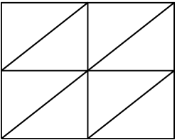
(a) Diagonal

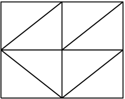
(b) Flipped

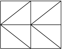
(c) Zigzag

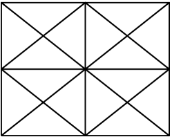
(d) Crisscross

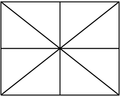
(e) Union Jack

Figure 1. Structured $2\times 2$ triangulations of the unit square.

	Diagonal	Flipped	Zigzag	Crisscross	Union Jack
$\sigma$	$0$	$0$	$0$	$n^{2}$	$n(n-2)/2$
$\dim\mathcal{N}_{h}$	$0$	$\begin{cases}(n/2-1)^{2}&r=1\\ 0&r=2,3\end{cases}$	$0$	$n^{2}$	$n(n-2)/2$

Table 1. The number of interior singular vertices $\sigma$ and the dimension of the space of spurious modes, $\dim\mathcal{N}_{h}$, for labeled families of $n\times n$ triangulations of the unit square, cf. Figure 1. For the flipped, zigzag and Union Jack meshes, $\dim\mathcal{N}_{h}$ is conjectural.

Recall that $\dim\mathcal{N}_{h}\geq\sigma$ for $r\geq 1$ and equality holds for $r\geq 4$. Qin proved that equality holds for $1\leq r\leq 3$ in the case of the diagonal and the crisscross meshes and numerically observed equality for the flipped mesh for $r=2$ [17]. Our own experiments show that equality holds for the zigzag and Union Jack meshes for $1\leq r\leq 3$. Equality also holds for the flipped mesh when $r=2,3$, but not for $r=1$. These results are summarized in the second row of Table 1.

We continue by studying the behaviour of the Brezzi inf-sup constants on the above triangulations. The cases $r=2,3$ are considered first, but we will return to the case $r=1$ below. For the Stokes equations, it is known that the diagonal and crisscross triangulation families exhibit very different behaviour for $r=2,3$ [17]. Namely, although there are non-trivial spurious modes on the crisscross triangulation family, the reduced Brezzi inf-sup constant is uniformly bounded. In contrast, for the diagonal family, the Brezzi inf-sup constant decays as approximately $\mathcal{O}(h)$. As the discretization is reduced stable for the Stokes equations on crisscross triangulations, it is also reduced stable for the mixed Laplacian. A natural question becomes whether the lack of stability on diagonal triangulations for the Stokes equations is also present for the mixed Laplacian.

In view of Lemma 3.1, we shall make an attempt at answering this question through a set of numerical experiments. For a given $r$ and a given $\mathcal{T}_{h}$, the smallest, and smallest non-zero, eigenvalue of (3.5) for $V=\mathcal{P}^{c}_{r}(\mathcal{T}_{h},\mathbb{V})$, $Q=\mathcal{P}_{r-1}(\mathcal{T}_{h})$ give the Brezzi inf-sup and reduced Brezzi inf-sup constant. These eigenvalues for the triangulation families considered, computed using LAPACK, SLEPc [11] and DOLFIN [12], are given for $r=1,2,3$ in Tables 2, 3 and 4. For the purpose of identifying spurious modes, eigenvalues below a threshold of $10^{-4}$ have been tabulated to zero.

	$\beta_{h}^{\operatorname{div}}$		$\tilde{\beta}_{h}^{\operatorname{div}}$ ($\dim\mathcal{N}_{h}$)
n	Diagonal	Zigzag	Flipped	Union Jack
4	0.847171	0.791967	0.945496 0(1)	0.976985 00(4)
6	0.716677	0.626865	0.945619 0(4)	0.976271 0(12)
8	0.605576	0.505968	0.947850 0(9)	0.975985 0(24)
10	0.517707	0.420180	0.946138 (16)	0.975847 0(40)
12	0.449060	0.357720	0.944833 (25)	0.975770 0(60)
14	0.394963	0.310731	0.943880 (36)	0.975724 0(84)
16	0.351684	0.274303	0.943142 (49)	0.975693 (112)

Table 2. The mixed Laplacian (reduced) Brezzi inf-sup constant for $\mathcal{P}^{c}_{1}(\mathcal{T}_{h};\mathbb{V})\times\mathcal{P}_{0}(\mathcal{T}_{h})$ on labeled structured families of triangulations $\mathcal{T}_{h}$. The dimension of the space of spurious modes in parenthesis if non-trivial.

	$\beta_{h}^{\operatorname{div}}$			$\tilde{\beta}_{h}^{\operatorname{div}}$ ($\dim\mathcal{N}_{h}$)
n	Diagonal	Zigzag	Flipped	Union Jack
4	0.975627	0.955956	0.943790	0.975628 0(4)
6	0.975600	0.952460	0.940480	0.975603 (12)
8	0.975595	0.951384	0.938717	0.975595 (24)
10	0.975594	0.950906	0.937684	0.975594 (40)
12	0.975594	0.950638	0.936992	0.975593 (60)
14	0.975593	0.950458

Table 3. The mixed Laplacian (reduced) Brezzi inf-sup constant for $\mathcal{P}^{c}_{2}(\mathcal{T}_{h};\mathbb{V})\times\mathcal{P}_{1}(\mathcal{T}_{h})$ on labeled structured families of triangulations $\mathcal{T}_{h}$. The dimension of the space of spurious modes in parenthesis if non-trivial.

	$\beta_{h}^{\operatorname{div}}$			$\tilde{\beta}_{h}^{\operatorname{div}}$ ($\dim\mathcal{N}_{h}$)
n	Diagonal	Zigzag	Flipped	Union Jack
4	0.972244	0.975594	0.975594	0.975594 0(4)
6	0.967304	0.975593	0.975593	0.975593 (12)
8	0.964845	0.975593	0.975593	0.975593 (24)
10	0.963412
12	0.962484

Table 4. The mixed Laplacian (reduced) Brezzi inf-sup constant for $\mathcal{P}^{c}_{3}(\mathcal{T}_{h};\mathbb{V})\times\mathcal{P}_{2}(\mathcal{T}_{h})$ on labeled structured families of triangulations $\mathcal{T}_{h}$. The dimension of the space of spurious modes in parenthesis if non-trivial.

For the diagonal meshes, the numerical experiments indicate that in contrast to Stokes, the mixed Laplacian Brezzi inf-sup constants are bounded from below for both $r=2,3$. For the flipped and zigzag meshes, experiments give similar results. Neither exhibits any spurious modes. Moreover, while the Brezzi inf-sup constant decays approximately as $\mathcal{O}(h)$ for the Stokes equations [17], it appears to be uniformly bounded for the mixed Laplacian. For the Union Jack family, the same experiment gives $n(n-2)/2$ spurious modes, but the reduced Brezzi inf-sup constant again seems to be uniformly bounded. In summary for $r=2,3$, the $\mathcal{P}^{c}_{r}(\mathbb{V})\times\mathcal{P}_{r-1}$ elements appear to be at least reduced stable for all the families considered.

With the discussion in Section 3.2 in mind, we also note that the Brezzi inf-sup constant converges to the exact value, given by (3.9), for some, but not all, of these meshes. For $r=2$, the Brezzi inf-sup constant seems to converge to the exact value on the diagonal meshes, but not on the flipped or the zigzag meshes. The situation is the opposite for $r=3$. There, the Brezzi inf-sup constant seems to converge to the exact value on the zigzag and flipped meshes, but not for the diagonal meshes.

The situation is different and more diverse in the lowest-order case: $r=1$. Boffi et al. proved that $\mathcal{P}^{c}_{1}(\mathbb{V})\times\mathcal{P}_{0}$ is in fact reduced stable for the mixed Laplacian on crisscross meshes [4]. It is not reduced stable for Stokes [17]. However, the element pair does not seem to be stable on diagonal meshes. The values in the first column of Table 2 indicate that the Brezzi inf-sup constant decays approximately as $\mathcal{O}(h)$. The same is the case for the zigzag meshes. For the Union Jack meshes, the situation is similar to the crisscross case. That is, the number of singular modes match the number of interior singular vertices and the reduced Brezzi inf-sup constant appears to be bounded from below. Finally, the flipped meshes display a surprising behaviour. There seem to be $(n/2-1)^{2}$ spurious modes, even though there are no singular vertices. This is the only case where we have observed $\dim\mathcal{N}_{h}>\sigma$. However, the reduced Brezzi inf-sup constant appears to be uniformly bounded.

4.2. Convergence

In the previous subsections, we have investigated the stability of the $\mathcal{P}^{c}_{r}(\mathbb{V})\times\mathcal{P}_{r-1}$ elements. Now, we proceed to examine the convergence properties of these elements on the diagonal meshes. Conjecturing that $\mathcal{P}^{c}_{r}(\mathbb{V})\times\mathcal{P}_{r-1}$ is stable on this mesh family for $r\geq 2$, in accordance with the numerical evidence presented above, the standard theory gives the error estimate

(4.2) $$\|u-u_{h}\|_{\operatorname{div}}+\|p-p_{h}\|_{0}\leq Ch^{r}\left(\|u\|_{r+1}+\|p\|_{r}\right).$$

For $r\geq 4$, the $L^{2}$ error estimate for the velocity can be improved [6, Theorem 12.4.9], thus yielding:

(4.3) $$\|u-u_{h}\|_{0}\leq Ch^{r+1}\|u\|_{r+1}.$$

In order to verify (4.2) and to see whether (4.3) appears to be attained for $r=2,3$, we consider a standard smooth exact solution to the Laplacian with pure Dirichlet boundary conditions:

(4.4) $$p(x,y)=\sin(2\pi x)\sin(2\pi y),\quad u=\operatorname{grad}p,\quad g=\operatorname{div}u.$$

The errors of the $\mathcal{P}^{c}_{r}(\mathbb{V})\times\mathcal{P}_{r-1}$ approximations for $1\leq r\leq 4$ on diagonal meshes can be examined in Figure 2. To compute the errors, both the source function $g$ and the exact solutions $u,p$ have been represented by sixth order piecewise polynomial interpolants $\Pi_{h}g$ and $\Pi_{h}u,\Pi_{h}p$, whereupon the errors have been calculated exactly (up to numerical precision).

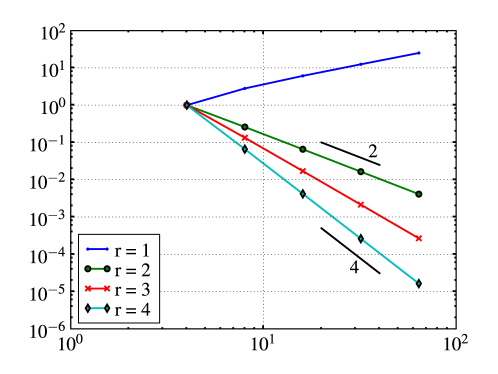
(a) Normalized pressure errors in $\|\cdot\|_{0}$.

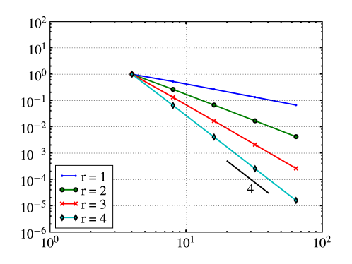
(b) Normalized velocity errors in $|\cdot|_{\operatorname{div}}$

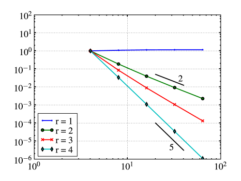
(c) Normalized velocity errors in $\|\cdot\|_{0}$

Figure 2. The errors of $\mathcal{P}^{c}_{r}(\mathbb{V})\times\mathcal{P}_{r-1}$ approximations for $r=1,2,3,4$ on diagonal meshes versus mesh number $n$. The errors have been normalized, that is, multiplied by the inverse of the error at the smallest mesh $n=4$.

For $r=1$, we observed the discretization to be unstable on diagonal meshes. As expected in this case, neither the pressure nor the velocity approximation seems to converge in the $L^{2}$ norm. This indicates that the estimates for the approximation error, based on the standard estimates and the decaying Brezzi inf-sup constant, cannot be improved. On the other hand, for $r>1$, we observed the method to be stable. For $r=2,3,4$, the orders of convergence in the $H(\operatorname{div})$ norm of the velocity and the $L^{2}$ norm of the pressure approximations are indeed optimal, as predicted by (4.2).

The situation seems different for the convergence of the velocity approximation in the $L^{2}$ norm. For $r\geq 4$, a convergence rate of order $r+1$ is predicted by (4.3). This is also observed for $r=4$ in Figure 2(c). On the other hand, for $r=2$ and $3$ the rate of convergence appears to be of order $r$, and thus one order suboptimal, indicating that the estimate (4.3) does not hold for $r<4$.

References

- [1] D. N. Arnold, R. S. Falk, and R. Winther. Finite element exterior calculus, homological techniques, and applications. Acta Numer., 15:1–155, 2006.
- [2] I. Babuška. The finite element method with Lagrangian multipliers. Numer. Math., 20:179–192, 1972/73.
- [3] D. Boffi, F. Brezzi, and M. Fortin. Finite elements for the Stokes problem. In Mixed Finite Elements, Compatibility Conditions, and Applications, volume 1939 of Lecture Notes in Mathematics, pages 45–100. Springer-Verlag, Berlin, 2008. Lectures given at the C.I.M.E. Summer School held in Cetraro, June 26–July 1, 2006, Edited by D. Boffi and L. Gastaldi.
- [4] D. Boffi, F. Brezzi, and L. Gastaldi. On the problem of spurious eigenvalues in the approximation of linear elliptic problems in mixed form. Math. Comp., 69(229):121–140, 2000.
- [5] D. Boffi, R. G. Duran, and L. Gastaldi. A remark on spurious eigenvalues in a square. Appl. Math. Lett., 12(3):107–114, 1999.
- [6] S. C. Brenner and L. R. Scott. The mathematical theory of finite element methods, volume 15 of Texts in Applied Mathematics. Springer, New York, third edition, 2008.
- [7] F. Brezzi. On the existence, uniqueness and approximation of saddle-point problems arising from Lagrangian multipliers. Rev. Française Automat. Informat. Recherche Opérationnelle Sér. Rouge, 8(R-2):129–151, 1974.
- [8] F. Brezzi, J. Douglas, Jr., and L. D. Marini. Two families of mixed finite elements for second order elliptic problems. Numer. Math., 47(2):217–235, 1985.
- [9] F. Brezzi and M. Fortin. Mixed and hybrid finite element methods, volume 15 of Springer Series in Computational Mathematics. Springer-Verlag, New York, 1991.
- [10] D. Chapelle and K.-J. Bathe. The inf-sup test. Comput. & Structures, 47(4-5):537–545, 1993.
- [11] V. Hernandez, J. E. Roman, and V. Vidal. SLEPc: a scalable and flexible toolkit for the solution of eigenvalue problems. ACM Trans. Math. Software, 31(3):351–362, 2005.
- [12] A. Logg, G. N. Wells, et al. DOLFIN. URL: http//www.fenics.org/dolfin/.
- [13] D. S. Malkus. Eigenproblems associated with the discrete LBB condition for incompressible finite elements. Internat. J. Engrg. Sci., 19(10):1299–1310, 1981.
- [14] K. A. Mardal, X.-C. Tai, and R. Winther. A robust finite element method for Darcy-Stokes flow. SIAM J. Numer. Anal., 40(5):1605–1631 (electronic), 2002.
- [15] J. Morgan and L. R. Scott. The dimension of the space of piecewise polynomials. Research Report UH/MD 78, University of Houston, Mathematics Department, 1990.
- [16] J. Morgan and R. Scott. A nodal basis for piecewise polynomials of degree . Math. Comput., 29:736–740, 1975.
- [17] J. Qin. On the Convergence of Some Low Order Mixed Finite Elements for Incompressible Fluids. PhD thesis, Penn State, 1994.
- [18] P.-A. Raviart and J. M. Thomas. A mixed finite element method for 2nd order elliptic problems. In Mathematical aspects of finite element methods (Proc. Conf., Consiglio Naz. delle Ricerche (C.N.R.), Rome, 1975), pages 292–315. Lecture Notes in Math., Vol. 606. Springer, Berlin, 1977.
- [19] L. R. Scott and M. Vogelius. Norm estimates for a maximal right inverse of the divergence operator in spaces of piecewise polynomials. RAIRO Modél. Math. Anal. Numér., 19(1):111–143, 1985.