ON THE EMERGENCE OF COLLECTIVE ORDER IN SWARMING SYSTEMS: A RECENT DEBATE

Abstract

In this work we consider the phase transition from ordered to disordered states that occur in the Vicsek model of self-propelled particles. This model was proposed to describe the emergence of collective order in swarming systems. When noise is added to the motion of the particles, the onset of collective order occurs through a dynamical phase transition. Based on their numerical results, Vicsek and his colleagues originally concluded that this phase transition was of second order (continuous). However, recent numerical evidence seems to indicate that the phase transition might be of first order (discontinuous), thus challenging Vicsek’s original results. In this work we review the evidence supporting both aspects of this debate. We also show new numerical results indicating that the apparent discontinuity of the phase transition may in fact be a numerical artifact produced by the artificial periodicity of the boundary conditions.

I Introduction

The collective motion of systems such as schools of fish, swarms of insects, or flocks of birds, in which hundreds or thousands of organisms move together in the same direction without the apparent guidance of a leader, is one of the most spectacular examples of large-scale organization observed in nature. From the physical point of view, there has been a drive to try to determine and understand the general principles that govern the emergence of collective order in these systems, in which the interactions between individuals are presumably of short-range. During the last 15 years, several models have been proposed to account for the large-scale properties of flocks and swarms. However, in spite of many efforts, the understanding of these general principles has remained elusive, partly due to the fact that the systems under study are not in equilibrium. Hence, the standard theorems and techniques of statistical mechanics that work well to explain the emergence of long range order in equilibrium systems, cannot be applied to understand the occurrence of apparently similar phenomena in large groups of moving organisms, or systems of self-propelled particles (SPP),as they have come to be known.

One of the simplest models conceived to describe swarming systems was proposed by Vicsek and his collaborators in 1995, Vicsek-PRL-95 . This model is “simple” in the sense that the interaction rules between the particles are quite easy to formulate and implement in computer simulations. However, it has been extremely difficult to characterize its dynamical properties either analytically or numerically. The central idea in Vicsek’s model is that at every time, each particle moves in the average direction of motion of its neighbors, plus some noise. In other words, each particle follows its neighbors. But the particles make “mistakes” when evaluating the direction of motion of their neighbors, and those mistakes are the noise. There might be several sources of noise. For instance, the environment can be blurred, and, consequently, the particles do not see very well the direction in which their neighbors are moving. We will call this type of noise extrinsic noise because it has to do with uncertainties in the particle-particle “communication” mechanism. On the other hand, it is possible to imagine the particles as having some kind of “free will”, so that even when they know exactly the direction of their neighbors, they may “decide” to move in a different direction. We will call this last type of noise the intrinsic noise because it can be thought of as being related to uncertainties in the internal decision-making mechanism of the particles.

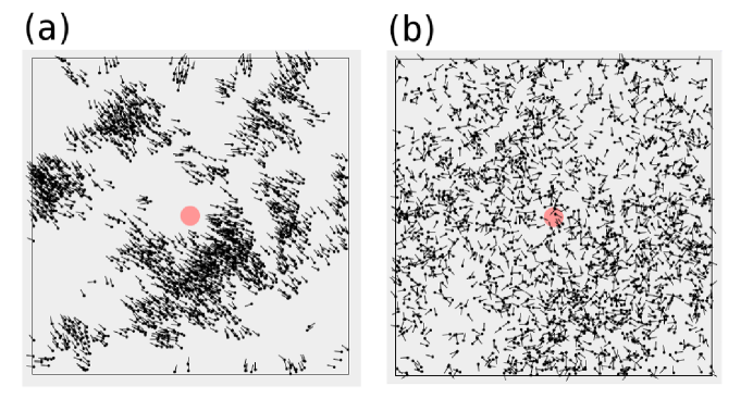
Figure 1: Snapshots of the Vicsek model. (a) For very small noise ($\eta=0.1$ ) all the particles move in the same direction. (b) For very large noise ($\eta=0.8$) the particles move in random uncorrelated directions. The shaded circle at the center of each frame indicates the size of the interaction vicinity. In both cases intrinsic noise was used. The other parameters are: Number of particles, $N=2000$; size of the box, $L=32$; particle speed, $v_{0}=0.05$; interaction radius, $r_{0}=1$.

In their original work, Vicsek et al. used intrinsic noise and showed that, when the noise amplitude is increased, the system undergoes a phase transition from an ordered state where all the particles move in the same direction, to a disordered state where the particles move in random uncorrelated directions (see Fig.1). Based on numerical results, this phase transition was thought to be of second order because it seemed to exhibit several of the characteristic properties of critical phase transitions, such as a non-trivial scaling behavior with the system size, divergence of the spatial correlation length, etc. However, in 2004 Grégoire and Chaté challenged these results, Chate-PRL-04 . By numerically analyzing large systems with many more particles than the ones studied by Vicsek and his colleagues, Grégoire and Chaté concluded that the phase transition is in fact of first order for both types of noise, intrinsic and extrinsic. This elicited a debate about the nature of the phase transition in the Vicsek model, namely, whether this phase transition is first order or second order. The existence of this debate, into which some other research groups have got involved, is indicative of the difficulties posed by the system, for not even such a fundamental property as the nature of the phase transition occurring in one of the simplest models of flocking, has been conclusively resolved.

The question as to whether the phase transition is first order or second order is not just of academic interest. Consider for instance a school of fish. For low values of the noise, the nature of the phase transition is irrelevant because the fish peacefully move in the same direction in a dynamical state far away from the phase transition. However, when the system is perturbed, for instance by a predator, the entire school of fish collectively responds to the attack: The school splits apart into smaller groups, which move in different directions and merge again later, confusing the predator. A possible hypothesis for this collective behavior to be possible is that, when attacked, the fish adjust their internal parameters to put the whole group close to the phase transition. If this phase transition is of second order, then the spatial correlation length diverges making it possible for the entire school to respond collectively. However, this collective response would be very difficult to mount if the phase transition was first order, since in such a case the spatial correlation length typically remains finite.

In this work we review the evidence supporting the two sides to this debate, i.e. the evidence supporting the continuous character of the phase transition and the evidence supporting its discontinuous character. It is important to mention that this is not a review on the general topic of animal flocking. For such a review, we refer the reader to Refs. Couzin-Krauze-03 -Parrish-BB-02 .

Here we focus only on the debate about the nature of the phase transition in the Vicsek model with intrinsic noise. In the next section we introduce the mathematical formulation of this model. In Sec. III we present the work supporting the conclusion that the phase transition is continuous, and in Sec. IV the evidence supporting the opposite conclusion. In Sec. V we present new evidence indicating that the discontinuous phase transition that has been reported may be an artifact of the boundary conditions, which in the numerical simulations performed so far have always been fully periodic. Finally, in Sec. VI we summarize the different aspects of this debate.

II The Vicsek Model

The model consists of $N$ particles placed on a two dimensional square box of sides $L$ with periodic boundary conditions. Each particle is characterized by its position $\vec{x}_{n}(t)$, and its velocity $\vec{v}_{n}(t)=v_{0}e^{i\theta_{n}(t)}$, which we represent here as a complex number to emphasize the velocity angle $\theta_{n}(t)$. All the particles move with the same speed $v_{0}$. What changes from one particle’s velocity to another is the direction of motion given by the angle $\theta_{n}(t)$. In order to state mathematically the interaction rule between the particles, let us define $U_{n}(r_{0};t)$ as the circular neighborhood or radius $r_{0}$ centered at $\vec{x}_{n}(t)$, and as $k_{n}(t)$ the number of particles withing this neighborhood (including the $n$-th particle itself). Let $\vec{V}_{n}(t)$ be the average velocity of the particles within the neighborhood $U_{n}(r_{0};t)$:

$$\vec{V}_{n}(t)=\frac{1}{k_{n}(t)}\sum_{\{j:\vec{x}_{j}\in U_{n}\}}\vec{v}_{j}(t).$$ (1)

With these definitions, the interaction between the particles with intrinsic noise is given by the simultaneous updating of all the velocity angles and all the particle positions according to the rule

$$\theta_{n}(t+\Delta t) = \mbox{Angle}\left[\vec{V}_{n}(t)\right]+\eta\xi_{n}(t),$$ (2a)

$$\vec{v}_{n}(t+\Delta t) = v_{0}e^{i\theta_{n}(t+\Delta t)},$$ (2b)

$$\vec{x}_{n}(t+\Delta t) = \vec{x}_{n}(t)+\vec{v}_{n}(t+\Delta t)\Delta t,$$ (2c)

where the function “Angle” is defined in such a way that for every vector $\vec{u}=ue^{i\theta}$ we have Angle$[\vec{u}]=\theta$. In addition, $\xi_{n}(t)$ is a random variable uniformly distributed in the interval $[-\pi,\pi]$, and the noise intensity $\eta$ is a positive parameter. Note that for $\eta=0$ the dynamics are fully deterministic and the system reaches a perfectly ordered state, whereas for $\eta\geq 1$ the particles undergo purely Brownian motion.

Analogously, the interaction rule with extrinsic noise is given by

$$\theta_{n}(t+\Delta t) = \mbox{Angle}\left[\vec{V}_{n}(t)+\eta e^{i\xi_{n}(t)}\right]$$ (3a)

$$\vec{v}_{n}(t+\Delta t) = v_{0}e^{i\theta_{n}(t+\Delta t)}$$ (3b)

$$\vec{x}_{n}(t+\Delta t) = \vec{x}_{n}(t)+\vec{v}_{n}(t+\Delta t)\Delta t$$ (3c)

where $\xi_{n}(t)$ and $\eta$ have the same meaning as before. Note that in Eq. (2a), the angle of the average velocity $\vec{V}_{n}(t)$ is computed and then a scalar noise $\eta\xi_{n}(t)$ is added to this angle. On the other hand, in Eq. (3a) a random vector $\eta e^{i\xi_{n}(t)}$ is added directly to the average velocity $\vec{V}_{n}(t)$, and afterwards the angle of the resultant vector is computed. Intuitively, we can interpret the average velocity $\vec{V}_{n}(t)$ as the signal that the $n$-th particle receives from its neighborhood, and the $Angle$ function as the particle’s decision-making mechanism. Therefore, in Eq. (2a) the particle clearly receives the signal from its neighborhood, computes the angle of motion, but then decides to move in a different direction. In contrast, in Eq. (3a) the particle receives a noisy signal from the neighborhood, but once the signal has been received, the particle computes the perceived angle and follows it.

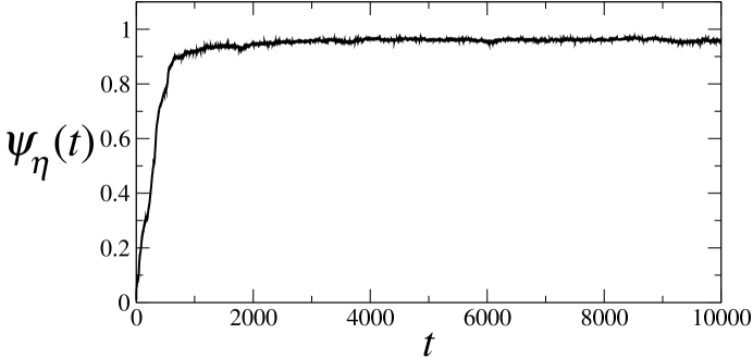
Figure 2: Time series of the order parameter $\psi_{\eta}(t)$. Starting from a random initial condition for which $\psi_{\eta}(0)\approx 0$, after a transient time (about 2000 time steps in this case), the system reaches a steady state reflected by stationarity of the order parameter. The simulation was carried out using intrinsic noise for a system with $N=2\times 10^{4}$, $\eta=0.1$, $v_{0}\Delta t=0.05$ and $r_{0}=0.4$.

At any time, the amount of order in the system is measured by the instantaneous order parameter defined as

$$\psi_{\eta}(t)=\frac{1}{Nv_{0}}\left|\sum_{n=1}^{N}\vec{v}_{n}(t)\right|,$$ (4)

where we have used the subscript $\eta$ to explicitly indicate that the order in the system depends on the noise intensity. After a transient time, the system reaches a steady state, as indicated in Fig. 2. In the stationary state, we can average $\psi_{\eta}(t)$ over noise realizations, or equivalently, over time. The stationary order parameter $\psi(\eta)$ is, thus, defined as

$$\psi(\eta)=\lim_{t\to\infty}\langle\psi_{\eta}(t)\rangle=\lim_{T\to\infty}\frac{1}{T}\int_{0}^{T}\psi_{\eta}(t)dt,$$ (5)

where $\langle\cdot\rangle$ denotes the average over realizations, whereas the average over time is given by the integral.

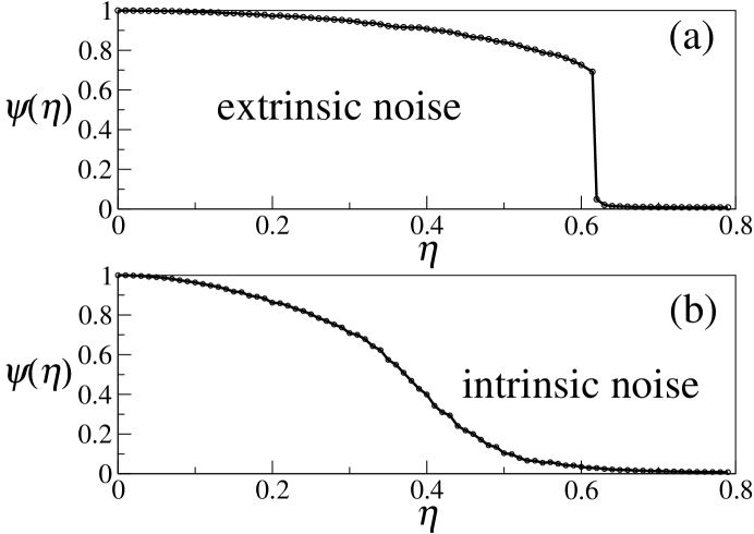
Figure 3: Phase transition diagram for a system with (a) extrinsic noise and (b) intrinsic noise. All the other parameters are the same for both systems: $N=2\times 10^{4}$, $L=32$, $v_{0}\Delta t=0.05$, and $r_{0}=0.4$. Note that in the extrinsic noise case the discontinuous phase transition is evident.

Fig. 3 shows typical phase transition curves for both types of noise, intrinsic and extrinsic. The discontinuous character of the phase transition for the extrinsic noise case is evident (Fig. 3a). As far as we can tell, there are no doubts that the phase transition is discontinuous in this case, and there is plenty of numerical and theoretical evidence supporting this finding, Chate-PRL-04 ; Aldana-PRL-07 ; albano-ijmpc-06 . In contrast, the phase transition shown in Fig. 3b for the case with intrinsic noise seems to be continuous. However, despite this apparent continuity, strong finite-size effects, reflected in the smoothness of the curve as $\psi\to 0$, may be hiding a possible discontinuity, as has been claimed by Grégoire and Chaté, Chate-PRL-04 . For some as yet unknown reason, these finite-size effects would be much stronger for the intrinsic noise than for the extrinsic noise, masking one discontinuity but not the other.

The numerical determination of the nature of a phase transition is a difficult task precisely because the finite-size effects can conceal any discontinuity either in the order parameter or in its derivatives. Several techniques to deal with phase transitions numerically have been developed Lee-PRL-90 -Binder-RPP-97 . For the particular case of the Vicsek model, and other closely related models, finite-size scaling analysis and dynamic scaling analysis Czirok-JPA-97 -Baglieto-PRE-08 , renormalization group Toner-PRL-95 -Tonner-AP-05 , mean-field theory Aldana-PRL-07 , Aldana-JSP-03 -Peruani-EPJ-08 , stability analysis Bertin-PRE-06 , and Binder cumulants Chate-PRL-04 ; Chate-comment ; Chate-PRE-08 , have been used. However, none of these techniques have determined conclusively the nature of the phase transition.

Raw parameters	Effective parameters
$N$ Number of particles $L$ Size of the box $v_{0}$ Particle speed $r_{0}$ Radius of interaction vicinity $\Delta t$ Integration time-step $\eta$ Noise intensity	$\rho=N/L^{2}$ Density $L^{\prime}=L/r_{0}$ Size of the box relative to the interaction radius $K=\rho(\pi r_{0}^{2})$ Average number of interactions per particle $l=(v_{0}\Delta t)/r_{0}$ Step size relative to the interaction radius $\eta$ Noise intensity

Table 1: Parameters in the Vicsek Model

Another problem for determining the nature of the transition, in addition to finite-size effects, is the existence of too many parameters. This makes the numerical exploration of the parameter space very difficult, and what is valid for one region may not be valid for a different region. For instance, for low densities and small particle speeds, the phase transition looks continuous for systems as large as the computer capacity permits one to analyze, Baglieto-PRE-08 ; Nagy-PA-07 . But for high densities, large system sizes and high speeds the phase transition appears to be discontinuous, Chate-PRL-04 ; Chate-PRE-08 . Table 1 lists all the parameters in the model. Of particular importance is $l=(v_{0}\Delta t)/r_{0}$, the step size relative to the interaction radius. When $l$ is small ($l<0.5$) we will say that the system is in the low-velocity regime. Otherwise, the system will be in the high-velocity regime.

III The Continuous Phase Transition

The first claim of the existence of a continuous phase transition in the self-propelled particles model was presented in Vicsek’s original work Vicsek-PRL-95 , which was entitled “Novel type of phase transition in a system of self-driven particles.” The adjective “novel” was used probably because this phase transition was not expected in view of the Mermin-Wagner theorem Mermin-PRL-66 , which asserts that in a low-dimensional (1D and 2D) equilibrium system with continuous symmetry and isotropic local interactions, there cannot exist a long-range order-disorder phase transition. Specifically, this theorem was proven having in mind Heisenberg and XY models of ferromagnetism. Vicsek’s model in 2D is similar to the XY model, but in the latter the particles are fixed to the nodes of a lattice, whereas in the former they are free to move throughout the system. It is the motion of the particles that gives rise to effective long-range spatial interactions among the particles in the system. These interactions are responsible for the onset of long-range order, producing the phase transition. We will come back to this point later, (see Sec.III.2).

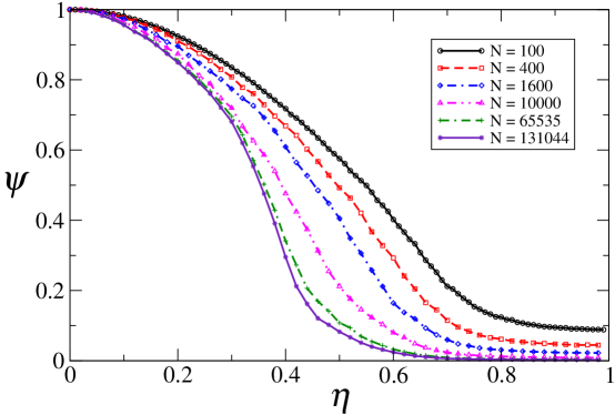
Figure 4: Phase transition in the Vicsek model for different system sizes. In all the cases the following parameters were used: $\rho=4$, $r_{0}=1$, and $v_{0}\Delta t=0.03$. Each point in each curve is the average of the instantaneous order parameter $\psi_{\eta}(t)$ over $10^{6}$ time steps.

Fig. 4 shows the phase transition for different system sizes, keeping the density constant, $\rho=4$. It should be emphasized that the curves shown in this figure correspond to a low-velocity regime in which the effective step-size $l=v_{0}\Delta t/r_{0}$ is small: $l=0.03$. This regime may be biologically plausible for systems such as flocks of birds, because birds can detect other birds that are far away compared to the distance traveled by each of them per unit of time. In Fig. 4, which is similar to the one originally published in Ref. Vicsek-PRL-95 but with more particles, one can observe that the phase transition remains continuous even for very large systems, up to $N=131044$. It is important to analyze very large systems because, as noted by Grégoire and Chaté Chate-PRL-04 ; Chate-comment ; Chate-PRE-08 , phase transitions occur in the thermodynamic limit defined as $N\to\infty$, $L\to\infty$, $\rho=const$. Using systems with different number of particles, up to $N=10^{5}$, Vicsek and his collaborators found numerically that the order parameter $\psi$ goes continuously to zero when the noise amplitude $\eta$ approaches a critical value $\eta_{c}$ from below as

$$\psi\approx(\eta_{c}-\eta)^{\beta},$$ (6)

with a non-trivial critical exponent $\beta=0.42\pm 0.03$, Czirok-JPA-97 ; Czirok-PA-00 . The critical value $\eta_{c}$ of the noise at which the phase transition seems to occur depends on the system size $L$ and on the density $\rho$. In this situation, finite-size scaling analysis can be done to check whether Eq. (6) can be expected to be valid in the thermodynamic limit, and to determine if a universal function $\tilde{\psi}(\eta/\eta_{c})$ exists such that the relationship $\psi(\eta)=\tilde{\psi}(\eta/\eta_{c})$ holds for any size $L$ and density $\rho$.

III.1 Finite-size scaling analysis

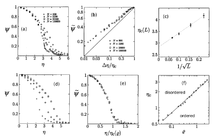
Figure 5: Scaling of the phase transition with the system size, [panels (a), (b) and (c)], and with the density $\rho$, [panels (d), (e) and (f)]. In the three top panels the density was kept constant, $\rho=2$, and the number of particles was increased. In the three bottom panels the system size was kept constant, $L=100$, and the density varied, ($\rho=4$ squares, $\rho=2$ diamonds, $\rho=0.5$ pluses). In all the cases the system was in the low-velocity regime $l=0.1$. The figures were taken from Ref. Czirok-JPA-97 . In that work the authors used $\eta\in[0,2\pi]$ and $\xi\in[-0.5,0.5]$, whereas here we use $\eta\in[0,1]$ and $\xi\in[-\pi,\pi]$. In (b) $\Delta\eta=\eta_{c}-\eta$.

In Refs. Czirok-JPA-97 ; Czirok-PA-00 , Vicsek and his group presented a finite-size scaling analysis showing that a universal function $\tilde{\psi}(\eta/\eta_{c})$ does indeed exist in the low-velocity regime. Fig. 5 shows how the phase transition scales with the system size $L$ and with the density $\rho$. From Figs. 5b and 5e it is clear that the order parameter computed for different system sizes and different densities, plotted as a function of $\eta/\eta_{c}$, falls onto the same universal curve $\tilde{\psi}(\eta/\eta_{c})$. Additionally, the critical value of the noise $\eta_{c}$ scales with the system size and the density respectively as $\eta_{c}\approx L^{-1/2}$, and $\eta_{c}\approx\rho^{\kappa}$, with $\kappa\approx 0.45$. A similar scaling behavior was found for systems in 1D and 3D Czirok-PA-99 ; Czirok-PRL-99 . It should be noted that the scaling behavior reported in Fig. 5 is consistent with of second-order phase transitions.

More recently, Baglieto and Albano performed a more thorough analysis Baglieto-PRE-08 , finding consistent evidence of a second order phase transition in the low-velocity regime (with $l=0.1$) by means of two independent approaches. The first approach is finite-size scaling analysis, in which they measure stationary properties of the system such as the order parameter $\psi(\eta)$ and the susceptibility $\chi=\langle\psi^{2}\rangle-\langle\psi\rangle^{2}$. They assume that the following scaling relations, which are well established in equilibrium systems, hold for the Vicsek model close to the phase transition:

$$\psi(\eta,L) \approx L^{-\beta/\nu}\tilde{\psi}\left((\eta_{c}-\eta)L^{1/\nu}\right),$$ (7)

$$\chi(\eta,L) \approx L^{\gamma/\nu}\tilde{\chi}\left((\eta_{c}-\eta)L^{1/\nu}\right).$$ (8)

where $\tilde{\psi}$ and $\tilde{\chi}$ are the (universal) scaling functions.

The second approach consists in performing short-time dynamic simulations and studying the results on the basis of dynamic-scaling theory, Zheng-IJMPB-98 . The main idea is to start out the dynamics from fully ordered ($\psi_{\eta}(t)=1$) and fully disordered ($\psi_{\eta}(t)\approx 0$) configurations, and analyze how the system relaxes in time to the steady state. Close to the phase transition, the relaxation from an ordered state is characterized by the scaling relations Zheng-IJMPB-98

$$\psi_{\eta}(t,L) \approx b^{-\beta/\nu}\hat{\psi}\left(b^{-z}t,b^{\nu}(\eta_{c}-\eta),b^{-1}L\right),$$ (9)

$$\chi_{\eta}(t,L) \approx b^{\gamma/\nu}\hat{\chi}\left(b^{-z}t,b^{\nu}(\eta_{c}-\eta),b^{-1}L\right).$$ (10)

where $z$ is the dynamic exponent, $b$ is an arbitrary scale factor, and $\hat{\psi}$ and $\hat{\chi}$ are the universal dynamic scaling functions. Additionally, it is known for equilibrium critical phenomena that the so-called hyperscaling relationship

$$d\nu-2\beta=\gamma,$$ (11)

must be satisfied Binney-92 . Baglieto and Albano showed numerically the validity of Eqs.(7)-(11) for systems of different sizes and densities, obtaining excellent agreement between the numerical results and the expected scaling relationships. Thus, when finite-size effects are taken into account in the Vicsek model with intrinsic noise and in the low-velocity regime, two independent methods, one static and the other dynamic, show consistency with a second-order phase transition.

III.2 Mean-field theory and network models

Figure 6: (a) Schematic representation of the long-range spatial correlations developed in time in the Vicsek model due to the motion of the particles. (b) A network model in which long-range interactions have been explicitly introduced via a small-world topology.

As mentioned above, the XY model is similar to the Vicsek model in that neighboring particles tend to align their “spins” (or velocities) in the same direction. However, it is well known that in the XY model, in which the particles do not move but are fixed to the nodes of a lattice, there is no long-range order-disorder phase transition Binney-92 . Thus, it is the motion of the particles in Vicsek’s model that enables the system to undergo a phase transition. What this motion actually does is to generate throughout time long-range spatial correlations between the particles. This is illustrated in Fig. 6a, in which two particles that at time $t_{0}$ do not interact, move and come together within the interaction radius at a later time $t_{1}$. In Refs. Aldana-PRL-07 and Aldana-JSP-03 a network model that attempts to capture this behavior is proposed. In this model the particles are placed on the nodes of a small-world network small-world , in which each particle has $K$ connections. The small-world property consists in that a fraction $p$ of these connections are chosen randomly whereas the other fraction $1-p$ are nearest-neighbor connections (see Fig. 6b). As in Vicsek’s and the XY models, each particle is characterized by a 2D vector (or “spin”), $\vec{v}_{n}(t)=v_{0}e^{i\theta_{n}(t)}$, of constant magnitude and whose direction changes in time according to Eqs. (2) and (1). However, in the network model the sum appearing in Eq. (1) is replace by the sum over the $K$ nodes connected to $\vec{v}_{n}$.

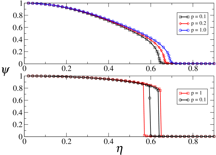
Figure 7: Phase transition in the network model with (a) intrinsic noise and (b) extrinsic noise. Note that in the first case the phase transition is continuous whereas in the second case it is discontinuous with a region of hysteresis. The network models can be considered as the mean-field description of the Vicsek model, especially for $p=1$. However, the same behavior is observed for any non-zero value of $p$, even for very small ones. For $p=0$ the small world network model is analogous to the XY model and no long-range order phase transition exists.

The network model described above differs from the Vicsek model in that the particles do not move, but are fixed to the nodes of a network. However, the long-range spatial correlations created by the motion of the particles in Vicsek’s model are mimicked in the network by the small-world topology, namely, by the $pKN$ random connections scattered throughout the system. Although the analogy is not exact, the network model can be considered as the mean-field version of Vicsek’s model, particularly when $p=1$, i.e. when the $K$ connections of each particle come randomly from anywhere in the system. In this case all spatial correlations are lost and the mean-field theory is exact. In Ref. Aldana-JSP-03 it is shown analytically that the network model with intrinsic noise and $p=1$ undergoes a second-order phase transition. In contrast, in Refs. Aldana-PRL-07 ; Pimentel-PRE-08 it is proved also analytically, and for $p=1$, that the network model with extrinsic noise exhibits a first-order phase transition. In Ref. Aldana-PRL-07 it was shown numerically that the network model with $p=1$ corresponds to the Vicsek model in the limiting case of very large particle speeds ($l\gg 1$). This is because of the fact that for very large particle speeds, two neighboring particles that at time $t_{0}$ are within the same interaction vicinity, because of the noise in the direction of motion of each particle, at the next time step $t_{0}+\Delta t$, they will end up far away from each other and interact with other particles. Thus, in the limit $v_{0}\to\infty$ of the Vicsek model, all spatial correlations are destroyed in one single time step, which is exactly the condition for the mean-field theory to be exact.

Numerical simulations show that for any $p\in(0,1]$, the phase transitions with intrinsic noise is continuous, whereas it is discontinuous with extrinsic noise (see Fig. 7). The results obtained with the network model indicate that the way in which the noise is introduced into the system can indeed change the nature of the phase transition. Therefore, the fact that the extrinsic noise produces a first-order transition cannot be used as supporting evidence for the continuous or discontinuous character of the transition with intrinsic noise.

The mean-field approach conveyed by the network model has been criticized on the basis that it neglects the coupling between local density and global order produced by the motion of the particles, Chate-comment . This coupling can generate spacial structures such as clusters of particles Huepe-PRL-04 , whereas in the mean-field theory one assumes that the system is spatially homogeneous. While this is true, is not clear how the coupling between order and density in the Vicsek model changes the nature of the phase transition.

III.3 Hydrodynamic models

For relatively large densities, one can imagine a flock as a continuum fluid in which neighboring fluid cells tend to align their momenta. This was the approach taken by Toner and Tu, Toner-PRL-95 -Tonner-AP-05 , who constructed a phenomenological hydrodynamic equation which has the same symmetries as the Vicsek model. Specifically, this equation includes isotropic short-range interactions, a self-propelled term, a stochastic driving force, and does not conserve momentum. Together with mass conservation, the system of hydrodynamic equations studied by Toner and Tu is

$$\partial_{t}\vec{v}+\lambda_{1}(\vec{v}\cdot\nabla)\vec{v}+\lambda_{2}(\nabla\cdot\vec{v})\vec{v}+\lambda_{3}\nabla(|\vec{v}|^{2}) = \alpha\vec{v}-\beta|\vec{v}|^{2}\vec{v}-\nabla P+D_{B}\nabla(\nabla\cdot\vec{v})+D_{T}\nabla^{2}\vec{v}+D_{2}(\vec{v}\cdot\nabla)^{2}\vec{v}+\vec{f},$$ (12)

$$P(\rho) = \sum_{n=1}^{\infty}\sigma_{n}(\rho-\rho_{0})^{n},$$ (13)

$$\partial_{t}\rho+\nabla\cdot(\vec{v}\rho) = 0,$$ (14)

where $\vec{v}$ is the velocity field, $\rho$ the density, $P$ the pressure, $\sigma_{n}$ are the coefficients in the pressure expansion, and $\vec{f}$ is a random Gaussian white noise which is equivalent to the noise term in the Vicsek model. Through a renormalization analysis of the above equations, Toner and Tu found scaling laws and relationships between different scaling exponents. Although the authors do not explicitly mention the nature of the phase transition, the characterization they present in terms of scaling laws and scaling exponents is, again, not inconsistent with a continuous phase transition in 2D.

Later, Bertin et al. derived an analogous hydrodynamic equation from microscopic principles incorporating only binary “collisions” of self-propelled particles with intrinsic noise into a Boltzmann equation, Bertin-PRE-06 . One of the advantages of this approach is that all the phenomenological coefficients appearing in Eq. (12), (the $\lambda$’s, $\alpha$, $\beta$, etc.), can be explicitly expressed in terms of microscopic quantities. The authors then show that the hydrodynamic equation has a homogeneous non-zero stationary solution that appears continuously as the density and the noise are varied. However, linear stability analysis shows that for this model, this homogeneous solution is unstable and therefore, the authors conclude, more complicated structures should appear in the system (such as bands or stripes, see Sec. V).

In any case, the evidence collected so far with hydrodynamic models of swarming, formulated along the same lines as the Vicsek model, while is not inconsistent with a second order phase transition, it has not been able either to shed light on the nature of the transition.

III.4 Models based on alignment forces

In a different type of swarming models the interactions between the particles are modeled through forces that tend to align the velocities of the interacting particles. Newton equations of motion are then solved for the entire system. Along these lines, Peruani et al. analyzed a system of over-damped particles whose dynamics is determined by the equations of motion Peruani-EPJ-08

$$\frac{d\vec{x}_{m}(t)}{dt} = v_{0}e^{i\theta_{m}(t)}$$ (15a)

$$\frac{d\theta_{m}(t)}{dt} = -\gamma\frac{\partial U_{m}(\vec{x}_{n},\theta_{n})}{\partial\theta_{m}}+\eta_{m}(t)$$ (15b)

where $\gamma$ is a relaxation constant, $\eta_{m}(t)$ is a Gaussian white noise (similar to the intrinsic noise in Vicsek’s model), and the potential interaction energy $U_{m}(\vec{x}_{n},\theta_{n})$ is given by

$$U_{m}(\vec{x}_{n},\theta_{n})=\sum_{|\vec{x}_{m}-\vec{x_{n}}|<r_{0}}\cos(\theta_{m}-\theta_{n}).$$

where $r_{0}$ is the radius of the interaction vicinity. In the limiting case $\gamma\to\infty$ of very fast angular relaxation, the above model is completely equivalent to the Vicsek model, Peruani-EPJ-08 .

Analogously, inspired by the migration of tissue cells (keratocytes), Szabó et al. formulated a model of over-damped swarming particles for which the dynamic equations of motion are Szabo-PRE-06

$$\vec{v}_{m}(t) = \frac{d\vec{x}_{m}(t)}{dt}=v_{0}\hat{n}_{m}(t)+\mu\sum_{n=1}^{N}\vec{F}(\vec{x}_{m},\vec{x}_{n})$$ (16a)

$$\frac{d\theta_{m}(t)}{dt} = \frac{1}{\tau}\arcsin\left(\left|\hat{n}_{m}(t)\times\frac{\vec{v}_{m}(t)}{|\vec{v}_{m}(t)|}\right|\right)+\eta_{m}(t)$$ (16b)

where $\theta_{m}$ is the angle of the unit vector $\hat{n}_{m}$, and $\eta_{m}(t)$ is again a Gaussian white noise. The interaction force $\vec{F}(\vec{x}_{m},\vec{x}_{n})$ depends piece-wise linearly on the distance $d_{mn}=|\vec{x}_{m}-\vec{x}_{n}|$. It is repulsive if $d_{mn}<R_{0}$, attractive if $r_{0}\leq d_{mn}\leq R_{1}$, and vanishes if $R_{1}<d_{mn}$. The explicit form of the force is

$$\vec{F}(\vec{x}_{m},\vec{x}_{n})=\hat{e}_{mn}\times\left\{\begin{array}[]{lcl}F_{r}\frac{d_{mn}-R_{0}}{R_{0}}&\mbox{ if }&d_{mn}<R_{0}\\ F_{a}\frac{d_{mn}-R_{0}}{R_{1}-R_{0}}&\mbox{ if }&R_{0}\leq d_{mn}\leq R_{1}\\ 0&\mbox{ if }&R_{1}<d_{mn}\end{array}\right.$$

where $\hat{e}_{mn}$ is the unit vector pointing from $\vec{x}_{n}$ to $\vec{x}_{m}$, and $F_{r}$ and $F_{a}$ are the magnitudes of maximum repulsion and maximum attraction, respectively.

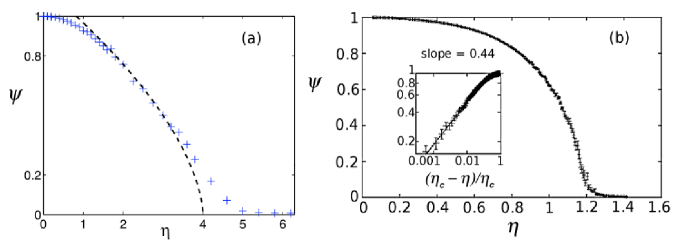
Figure 8: Phase transitions in swarming models based on alignment forces with intrinsic noise. (a) Order parameter as a function of the noise intensity for the model given in Eqs. (15). The dashed curve is the mean-field prediction whereas the symbols correspond to numerical simulations. (b) Phase transition for the model given in Eqs. (16). The data were obtained from numerical simulations. In both cases the phase transition is continuous. The figures (a) and (b) were taken (with small modifications to make the labels clearer) from Refs. Peruani-EPJ-08 and Szabo-PRE-06 , respectively.

In the two models described above, the forces between neighboring particles tend to align their velocities if the particles are withing the specified region, and in both models the particles are subjected to intrinsic noise. Interestingly, numerical simulations show that the states of collective order in these two models appear continuously through a second order phase transition, as Fig. 8 illustrates.

IV The Discontinuous Phase Transition

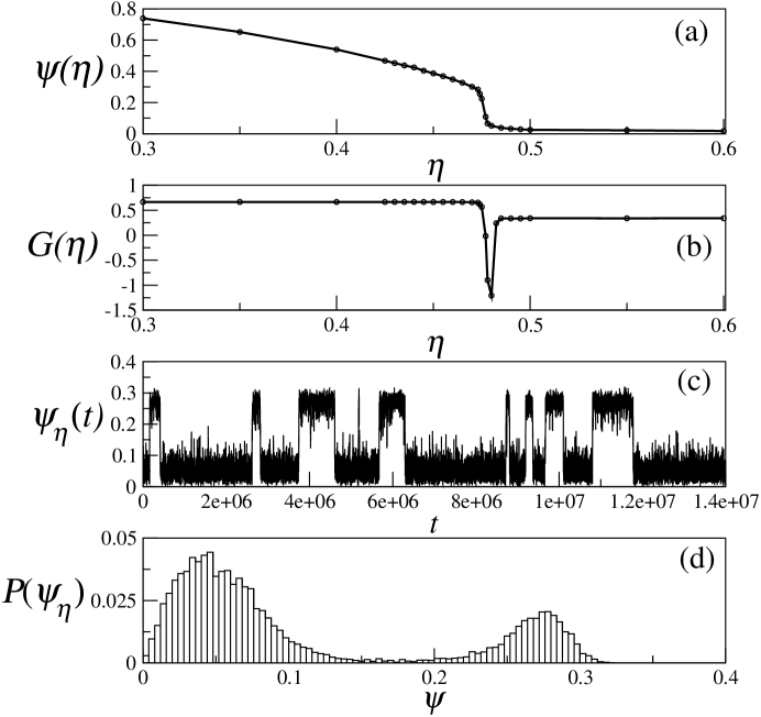
Figure 9: Evidence of the discontinuous character of the phase transition in the Vicsek model with intrinsic noise, for as system with $N=131072$ particles, $L=256$, and $l=0.5$. (a) Order parameter $\psi$ as a function of the noise intensity $\eta$. In this case the order parameter decays to zero discontinuously around the critical value $\eta_{c}\approx 0.478$. (b) Binder cumulant $G$ as a function of $\eta$. Note the sharp minimum of the Binder cumulant close to the phase transition. (c) Time series of the instantaneous order parameter $\psi_{\eta}(t)$ for $\eta=0.475$ (very close to the phase transition). This time series exhibits bistability, which is characteristic of phase coexistence in a first-order phase transition. (d) Probability distribution function $P(\psi_{\eta})$ of the instantaneous order parameter $\psi_{\eta}(t)$. This PDF is bimodal because of the bistability of the time series. In (a) and (b) each data point is the average of $\psi_{\eta}(t)$ over $2\times 10^{7}$ time steps.

The first evidence for the discontinuous character of the phase transition in the Vicsek model with intrinsic noise appeared in Ref. Chate-PRL-04 , and it was later reinforced in Ref. Chate-PRE-08 . In that work the authors studied very large systems in the high-velocity regime $l\geq 0.5$, . Fig. 9 summarizes this evidence for a large system, with $N=131072$ particles, $L=256$, and $l=0.5$. This system is similar to one of the systems used by Grégoire and Chaté in Ref. Chate-PRL-04 to demonstrate the discontinuity of the phase transition with intrinsic noise. It is clear from Fig. 9a that the order parameter undergoes an apparently discontinuous phase transition around a critical value $\eta_{c}=0.478$. Such a discontinuity is confirmed by the Binder cumulant $G(\eta)$, defined as

$$G(\eta)=1-\frac{\langle\psi_{\eta}^{4}\rangle}{3\langle\psi_{\eta}^{2}\rangle^{2}}.$$ (17)

The Binder cumulant, which is closely related to the Kurtosis, can intuitively be interpreted as a measure of how much a probability distribution function (PDF) differs from a Gaussian, particularly concerning the “peakedness” of the distribution. It was introduced by Binder as a means to determine numerically the nature of a phase transition, Binder-RPP-87 ; Tsai-BJP-98 . The idea behind this measure is that in a first-order phase transition, typically two different metastable phases coexist. Throughout time, the system transits between these two phases and consequently the time series of the order parameter shows a bistable behavior, as it is illustrated in Fig. 9c. The PDF $P(\psi_{\eta})$ of this time series is then bimodal, reflecting the coexistence of the two different phases and the transit of the system between them (see Fig. 9d). Because of this bimodality of $P(\psi_{\eta})$, which occurs only close to the phase transition, the Binder cumulant has a sharp minimum, as it is actually observed in Fig. 9b. On the other hand, far from the phase transition, either in the ordered regime or in the disordered one, $P(\psi_{\eta})$ is unimodal and rather similar to a Gaussian, for which the Binder cumulant is constant. It is only close to a discontinuous phase transition that $P(\psi_{\eta})$ becomes bimodal, thus deviating from a Gaussian, and the Binder cumulant $G(\eta)$ exhibits a sharp minimum. This is the strongest evidence presented by Grégoire and Chaté in favor of a discontinuous phase transition in the Vicsek model with intrinsic noise, Chate-PRL-04 ; Chate-PRE-08 . They also analyzed variations of this model, for instance by introducing cohesion or substituting the intrinsic noise by extrinsic noise. However, the mean field network models presented in Sec. III.2 show that the results obtained for one type of noise cannot be extrapolated to a different type of noise. Thus, in this section we will focus on the intrinsic noise case.

It should be emphasized that the discontinuous behavior displayed in Fig. 9 is observed only in the high velocity regime. Indeed, it is apparent from Fig. 4 that in the low-velocity regime $l=0.03$, the order parameter $\psi(\eta)$ does not exhibit any discontinuity even for a large system with $N=131044$ and $L=181$, (comparable in size to the one used in Fig. 9). It could be possible that the phase transition changes from continuous to discontinuous across the parameter space. However, the authors of Refs. Chate-PRL-04 and Chate-PRE-08 claim that this does not happen. They state that all phase transitions occur in the thermodynamic limit, and if we were able to explore very large systems, then the phase transition in the Vicsek model with intrinsic noise would turn out to be discontinuous for any values of the parameters, Chate-comment .

Another important aspect of the discontinuous phase transition shown in Fig. 9a is the absence of hysteresis. Indeed, our numerical simulations show that for this system it is irrelevant to start out the dynamics from ordered or from disordered states, because in either case the curve displayed in Fig. 9a is obtained. This is in marked contrast with the hysteresis commonly observed in usual first-order phase transitions, as the one depicted in Fig. 7b, which corresponds to the extrinsic noise dynamics and therefore is undoubtedly first order and in accord with the mean-field analytical results (see Sec. III.2). In the next section we present evidence indicating that the discontinuity of the phase transition observed in Fig. 9 may in fact be an artifact of the periodic boundary conditions, as first proposed by Nagy et al, Nagy-PA-07 .

V The Effect of the Boundary Conditions

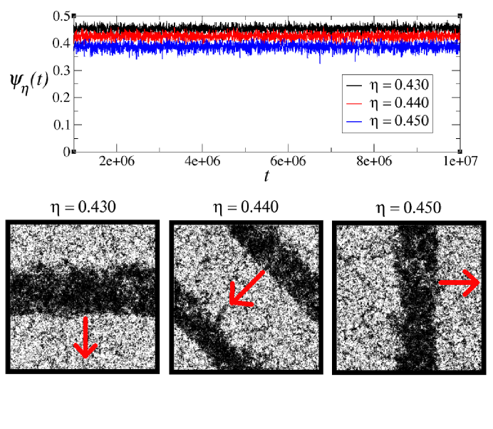
Figure 10: Traveling bands in the Vicsek model with intrinsic noise. The top panel shows the time series of the order parameter for three different values of the noise intensity $\eta$. The images at the bottom are snapshots of the system corresponding to each of the three values of $\eta$ used. The arrows indicate the direction of motion of the bands.

In a recent paper Nagy-PA-07 , Nagy, Daruka and Vicsek pointed out the formation of traveling bands in the high velocity regime. In Fig. 10 we show these bands for three different values of the noise intensity $\eta$ and for the same system used to compute the phase transition in Fig. 9. Note that the three values of $\eta$ in Fig. 10, ($\eta=0.430$, $\eta=0.440$ and $\eta=0.450$), correspond to the ordered regime, quite far from the transition, which occurs around $\eta_{c}\approx 0.478$. Interestingly, the bands always wrap around tightly in a periodic direction, which for simple shapes is usually either perpendicular or parallel to a boundary of the periodic box, or along a diagonal. In the ordered regime, the bands are very stable. Once they form, they may travel for extremely long times in the same direction (as shown in Fig. 10, the motion of the bands, indicated by the arrow, is perpendicular to themselves). In Ref. Nagy-PA-07 the authors also use hexagonal boxes with periodic boundary conditions, and the bands again always form parallel to the boundaries of the hexagon or to its diagonals.

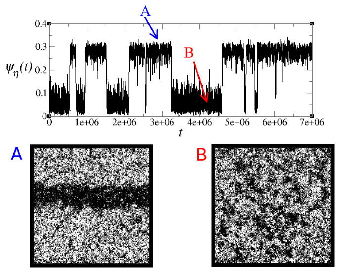
Figure 11: Bistable time series of the order parameter at a noise intensity $\eta=0.475$ for the same system as in Fig. 9. This value is very close to the critical value $\eta_{c}=0.478$. The bottom figures are snapshots of the system at the times indicated by the points A and B in the time series. The apparent bistability of the order parameter indicates the formation and destruction of the bands.

When the value of $\eta$ approaches the critical value $\eta_{c}$, the bands become unstable: They appear and disappear intermittently throughout the temporal evolution of the system. Fig. 11 shows the time series of the order parameter for the same system used in Fig. 9, at a noise intensity $\eta=0.475$, i.e. very close to the discontinuity. The time series shows that the order parameter “jumps” between two rather different values. These jumps give rise to the bimodality of the order parameter, which, according to the interpretation presented in the previous section, indicates phase coexistence. A close inspection of the spatial structure of the system reveals that such bistability is produced by the creation and destruction of the traveling bands, as the two snapshots in Fig. 11 indicate. Thus, as time passes, the system transits from spatially homogeneous states to states characterized by traveling bands. The authors of Ref. Chate-PRE-08 interpreted these bands as one of the two metastable phases, which coexists with a more or less homogeneous background of diffusive particles (the other metastable phase). However, Vicsek and his group retorted that the formation of traveling bands is not an intrinsic property of the system, but, rather, an artifact of the periodic boundary conditions.

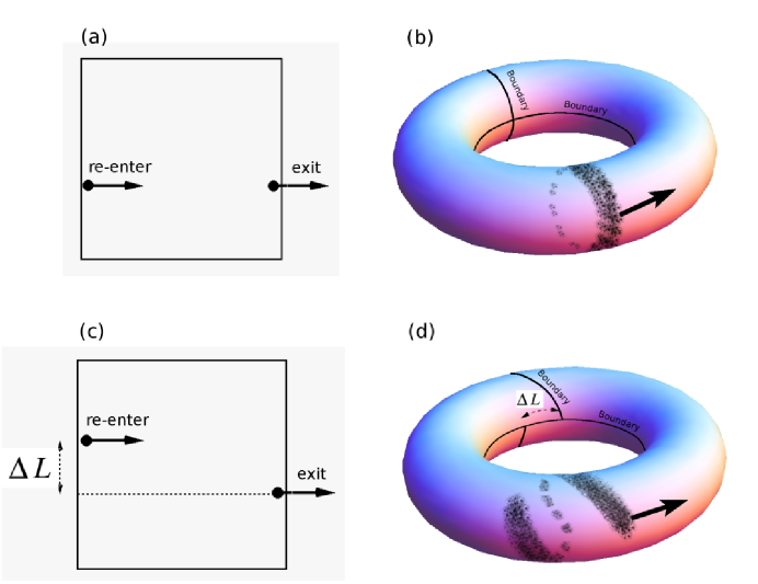
Figure 12: (a) In the original Vicsek model one implements periodic boundary conditions: If a particle exits through one side of the box, it re-enters through the opposite side at a specular position. (b) The periodic boundary conditions induce a toroidal topology that favors the formation of bands (closed rings) moving on the torus’ surface. (c) Shift $\Delta L$ in the boundary conditions. The shift is implemented in the four sides of the box, which breaks the toroidal symmetry of the dynamics and makes the closed ring structures unstable, as it is illustrated in (d).

It is a very common resource in numerical simulations of physical systems to use periodic boundary conditions as way to represent an infinite homogeneous space and mitigate boundary effects. In Vicsek’s model the particles move in a box of sides $L$. If a given particle exits the box through one of the sides, it is re-injected into the system through the opposite side at a specular position (see Fig. 12a). Under these circumstances, the real geometry of the box is that of a torus, and the motion of the particles takes place on its surface. The toroidal topology induced by the periodic boundary conditions clearly favors the formation of bands, which in fact are closed stable rings moving on the surface of the torus, as is illustrated in Fig. 12b. However, there is no reason whatsoever to re-inject the particles at specular positions of the box. Rather, it is possible to re-inject the particles at positions that are shifted a distance $\Delta L$ with respect to the specular position, as is done in Fig. 12c. By doing so, the toroidal topology is broken and the formation of bands (closed rings) is not longer stabilized by (toroidal) periodic boundary conditions. The idea is schematically illustrated in Fig. 12c, although the real situation is more complicated because the shift $\Delta L$ is implemented in the four sides of the box (see the Appendix). This shift, which we will refer to as the boundary shift, does not affect the homogeneity of the system, as all the particles are subjected to it when they hit the boundary. Interestingly, when the shift is implemented, the discontinuity of the phase transition reported in Refs. Chate-PRL-04 and Chate-PRE-08 , and reproduced here in Fig. 9, seems to disappear.

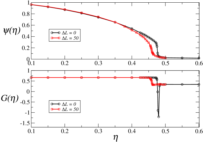
Figure 13: Effect of the boundary shift $\Delta L$ on the phase transition in the Vicsek model with intrinsic noise. (a) Order parameter as a function of the noise intensity for a system with no shift (black curve with circles), and for a system with a boundary shift $\Delta L=0.2L$ (red curve with squares). Note that the apparent discontinuity of the phase transition for the system with periodic boundary conditions disappears when the shift is introduced. (b) Binder cumulant corresponding to the two curves displayed in (a). The sharp negative peak disappears for the system with non-zero boundary shift. The curves were computed for systems with $N=131072$, $L=256$, and $l=0.5$. Every data point is the average of $\psi_{\eta}(t)$ over $2\times 10^{7}$ time-steps.

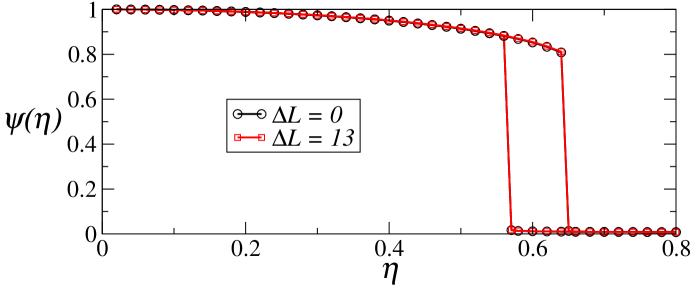
Figure 14: Phase transition in the Vicsek model with extrinsic noise for systems with $N=80000$, $L=64$, and $l=0.5$. The black circles correspond to fully periodic boundary conditions, i.e. $\Delta L=0$, whereas the squares correspond to a boundary shift $\Delta L=0.2L$. It is clear that in this case the boundary shift does not change the phase transition, which is undoubtedly discontinuous.

Fig. 13a shows the phase transition for the same system as the one used in Fig. 9, but this time comparing the two cases: With fully periodic boundary conditions, i.e. $\Delta L=0$ (black curve with circles), and with a non-zero boundary shift $\Delta L=0.2L$ (red curve with squares). In Fig. 13b the corresponding Binder cumulants are reported. We choose $\Delta L=0.2L$ because this is approximately the width of the bands close to the transition (see snapshot A in Fig. 11). It is clear from Fig. 13 that the introduction of the boundary shift eliminates the discontinuity of the phase transition, making it continuous. Note that the sharp peak in the Binder cumulant also disappears. It could be argued, then, that if the phase transition was intrinsically discontinuous, the introduction of the boundary shift should not change its character. This is indeed what happens in the Vicsek model with extrinsic noise with a boundary shift $\Delta L=0.2L$, as illustrated in Fig. 14. In such case, of course, the introduction of the boundary shift does not change the appearance of the phase transition. The above results give support to the claim that the apparent discontinuous character of the phase transition in the intrinsic noise case may indeed be an artifact of the topology induced by the periodic boundary conditions, as Vicsek and his colleagues had already suggested, Nagy-PA-07 .

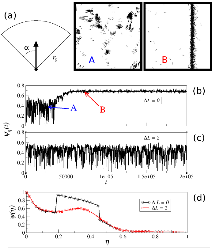
Figure 15: Phase transition in a variation of the Vicsek model with $N=1600$, $L=20$ and $l=0.03$. (a) The interaction vicinity is a circular cone of radius $r_{0}=1$ and angular amplitude $2\alpha$, centered at the particle’s velocity. (b) Time series of the order parameter for $\alpha=0.4\pi$ and $\eta=0.44$, with fully periodic boundary conditions ($\Delta L=0$). Note that after a transient time, the particles aggregate in a very dense band parallel to the boundary. The snapshots A and B correspond to the points signaled with the arrows in the time series. (c) The same as in the previous panel but now with a boundary shift $\Delta L=0.1L$. (d) Phase transition diagram with (red curve) and without (black curve) boundary shift. Note the discontinuities produced by the periodic boundary conditions.

A more dramatic effect of the periodic boundary conditions on the phase transition can be observed in a simple variation of the Vicsek model, for which it is not necessary to analyze very large systems. In this variation, the particles have a “vision angle”. In other words, the interaction region of each particle is no longer a full circle surrounding it, but only a circular cone of amplitude $2\alpha$ centered at the particle’s velocity, as illustrated in Fig. 15a. All the other aspects of the interaction are as in Vicsek’s model, only the form of the interaction vicinity is changed. In what follows we consider such a system with intrinsic noise and $N=1600$, $L=20$, $l=0.03$ (low-velocity regime), and $\alpha=0.4\pi$. For periodic boundary conditions and some values of the intrinsic noise, after a transient time the particles form very dense bands, as shown in Fig. 15b and the corresponding snapshots. Actually, as time goes by, the system transits back and forth, from configurations like the one depicted in snapshot A, to configurations with bands, as the one shown in snapshot B. Those bands produce two discontinuities in the curve of the order parameter, which is plotted in Fig. 15d (black curve with circles). Interestingly, these discontinuities do not occur close to the phase transition (which in this case seems to happen around $\eta_{c}\approx 0.6$), but well into the ordered phase. On the other hand, Fig. 15c shows the time series of the order parameter when a boundary shift $\Delta L=0.1L$ is introduced. Note that in this case the order parameter does not reflect the transit of the system between any two phases. This is because with the boundary shift the bands no longer form and the two discontinuities in the phase transition curve disappear, as is apparent from Fig. 15d (red curve with squares).

This variation of the Vicsek model clearly demonstrates that the periodic boundary conditions can have a dramatic effect on the system dynamics, producing artificial discontinuities in the order parameter that would not necessarily be present in an infinite system with no boundaries.

VI Summary

In this work we have presented much of the evidence offered in support of two distinct points of view, at odds with each other, about the nature of the phase transition in the Vicsek model of self-propelled particles with intrinsic noise. On the one hand, there is theoretical and numerical evidence indicating that such a phase transition is continuous. This evidence comes from several fronts: From the numerical side, finite-size scaling analysis and dynamic scaling analysis performed for systems operating in the low-velocity regime, have yielded results consistent with a continuous phase transition. These numerical techniques show scaling behavior of the order parameter with the size of the system and with the density, for systems as large as the computer capacity allows one to analyze. Additionally, the hyperscaling relationship between the critical exponents has been confirmed within numerical accuracy. This scaling behavior is consistent with what is known for second order phase transitions in equilibrium systems. From the theoretical side, analytic calculations unambiguously show that the mean-field version of the Vicsek model with intrinsic noise undergoes a second-order phase transition. Furthermore, swarming models based on alignment forces, (rather than on kinematic rules), also exhibit continuous phase transitions when the intrinsic noise is used.

On the other hand, there is direct numerical evidence suggesting that the phase transition is discontinuous in very large systems operating in the high-velocity regime. In addition to a clear discontinuity in the phase transition curve for these large systems, this point of view is supported by an apparent bistability of the order parameter close to the phase transition, and the corresponding bimodality of its PDF signaled by a “dip” of the Binder cumulant. Such a scenario is characteristic of phase coexistence in first-order transitions.

However, numerical computations performed for systems comparable in size to those used to demonstrate that the phase transition is discontinuous, suggest that the apparent discontinuity is an artifact of the toroidal topology induced by the periodic boundary conditions. For, when the boundary conditions are “shifted” in order to break the periodicity, and hence the toroidal symmetry, the discontinuity disappears. This effect is enhanced when the particles have a limited vision angle.

Determining the nature of the phase transition in the Vicsek model with intrinsic noise is important, among other things, for understanding the physical principles through which collective order emerges in swarms and flocks, and more generally, in systems out of equilibrium. Despite the efforts of many groups during the last decade, nobody has said the last word about the onset of collective order in swarming systems. This remains an open problem.

Appendix A Boundary shift

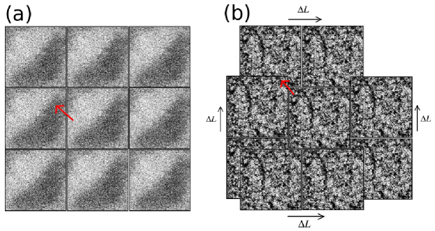
Figure 16: (a) A system with periodic boundary conditions. This is equivalent to making infinite copies of the central box and covering homogeneously the space with them. (b) A system with boundary shift. Note that the shifted boxes overlap at the corners of the central box.

In this appendix we explain how the boundary shift $\Delta L$ was implemented in our numerical simulations. Let us start with a system with periodic boundary conditions, as in Fig. 12a. Using periodic boundary conditions is equivalent to making infinite copies of the original system, and covering homogeneously all the space with these copies. This is illustrated in Fig. 16a, where a central box has been “cloned” several times. A particle exiting the central box just re-enters into it at a position equivalent to the one it would have in the adjacent box, and so on.

On the other hand, Fig. 16b shows how the boundary shift $\Delta L$ is implemented. The copies of the central box have been shifted around it the same positive distance $\Delta L$ in both the horizontal and the vertical directions. In this case, the space is not cover homogeneously because the shifted boxes overlap, as it is clearly seen in Fig. 16b. However, this overlap is important only for particles exiting the central box from the corners (as the one signaled with an arrow), because such a particle does not “know” what box to go to. This overlapping mixes the particles exiting from the corners in a way which is different from the natural motion of the particles located at the bulk of the system. Thus, the boundary shift $\Delta L$ introduces inhomogeneities in the “tiling” of the space. These inhomogeneities occur in regions of size $v_{0}\Delta t$ around the corners of the central box. Therefore, if $(v_{0}\Delta t)/L\ll 1$, as it has been the case in all the simulations carried out in this work, the inhomogeneities generated by the boundary shift should be negligible. In our simulations, when a particle exits the central box from one of the corners, it randomly chooses one of the two overlapping boxes to be re-injected into it.

References

- (1) T. Vicsek, A. Czirók, E. Ben-Jacob, I. Cohen and O. Shochet. Phys. Rev. Lett 75, 1226 (1995).
- (2) G. Grégoire and H. Chaté. Phys. Rev. Lett. 92, 025702 (2004).
- (3) I.D. Couzin and J. Krause. Adv. Study Behav. 32, 1 (2003).
- (4) D.J.T. Sumpter Phil. Trans. R. Soc. B 361, 5 (2006).
- (5) I. Giardina. HFSP Jour. 2, 205 (2008).
- (6) J.K. Parrish, S.V. Viscido and D. Grünbaum. Biol. Bull. 202, 296 (2002).
- (7) M. Aldana, V. Dossetti, C. Huepe, V.M. Kenkre and H. Larralde. Phys. Rev. Lett. 98, 095702 (2007).
- (8) G. Baglietto and E.V. Albano. Int. Jour. Mod. Phys. C 17, 395 (2006).
- (9) J. Lee and J.M. Kosterlitz. Phys. Rev. Lett. 65, 137 (1990).
- (10) K. Binder and D.P. Landau. Phys. Rev. B 30, 1477 (1984).
- (11) M.S.S. Challa, D.P. Landau and K. Binder. Phys. Rev. B 34, 1841 (1986).
- (12) K. Binder. Rep. Prog. Phys. 50, 783 (1987).
- (13) K. Binder. Rep. Prog. Phys. 60, 487 (1997).
- (14) A. Czirók, H.E. Stanley and T. Vicsek. J. Phys. A 30, 1375 (1997).
- (15) A. Czirók and T. Vicsek. Physica A 281, 17 (2000).
- (16) A. Czirók, M. Vicsek and T. Vicsek. Physica A 264, 299 (1999).
- (17) A. Czirok, A.-L. Barabási and T. Vicsek. Phys. Rev. Lett. 82, 209 (1999).
- (18) G. Baglieto and G.V. Albano. Phys. Rev. E 78, 021125 (2008).
- (19) J. Toner and Y. Tu. Phys. Rev. Lett. 75, 4326 (1995).
- (20) J. Toner and Y. Tu. Phys. Rev. E 58, 4828 (1998).
- (21) Y. Tu. Physica A 281, 30 (2000).
- (22) J. Toner, Y. Tu and S. Ramaswamy. Ann. Phys. 318, 170 (2005).
- (23) M. Aldana and C. Huepe. J. Stat. Phys. 112, 135 (2003).
- (24) J.A. Pimentel, M. Aldana, C. Huepe and H. Larralde. Phys. Rev. E 77, 061138 (2008).
- (25) F. Peruani, A. Deutsch and M. Bär. Eur. Phys. J. Special Topics 157, 111 (2008).
- (26) E. Bertin, M. Droz and G. Grégoire. Phys. Rev. E 74, 022101 (1006).
- (27) H. Chaté, F. Ginelli and G. Grégoire. Phys. Rev. Lett. 99, 229601 (2007).
- (28) H. Chaté, F. Ginelli, G. Grégoire and F. Raynaud. Phys. Rev. E 77, 046113 (2008).
- (29) M. Nagy, I. Daruka and T. Vicsek. Physica A 373, 445 (2007).
- (30) N.D. Mermin and H. Wagner. Phys. Rev. Lett. 22, 1133 (1966).
- (31) M. Ballerini, N. Cabibbo, R. Candelier, et al. Proc. Natl. Acad. Sci. USA 105, 1232 (2008).
- (32) B. Zheng. Int. J. Mod. Phys. B 12, 1419 (1998).
- (33) J.J. Binney, N.J. Dowrick, A.J. Fisher and M.E.J. Newman. The Theory of Critical Phenomena: An Introduction to the Renormalization Group (Oxford University Press, New York, 1992).
- (34) S.H. Strogatz. Nature 410, 268 (2001).
- (35) C. Huepe and M. Aldana. Phys. Rev. Lett. 92, 168701 (2004).
- (36) B. Szabó, G.J. Szöllösi, B. Gönci, Zs. Jurányi, D. Selmeczi and T. Vicsek. Phys. Rev. E 74, 061908 (2006).
- (37) J. Buhl, D.J.T. Sumpter, I.D. Couzin, et al. Science 312, 1402 (2006).
- (38) S.J. Simpson, G.A. Sword, P.D. Lorch and I.D. Couzin. Proc. Natl. Acad. Sci. USA. 103, 4152 (2006).
- (39) S.-H. Tsai and S.R. Salinas. Braz. Jour. Phys. 28, 58 (1998).