Quantum Reading of Digital Memories

Abstract

We consider a basic model of digital memory where each cell is composed of a reflecting medium with two possible reflectivities. By fixing the mean number of photons irradiated over each memory cell, we show that a non-classical source of light can retrieve more information than any classical source. This improvement is shown in the regime of few photons and high reflectivities, where the gain of information can be surprising. As a result, the use of quantum light can have non-trivial applications in the technology of digital memories, such as optical disks and barcodes.

In recent years, non-classical states of radiation have been exploited to achieve marvellous results in quantum information and computation NielsenBook ; BraREV ; BraREV2 ; GaussSTATES . In the language of quantum optics, the bosonic states of the electromagnetic field are called “classical” when they can be expressed as probabilistic mixtures of coherent states. Classical states describe practically all the radiation sources which are used in today’s technological applications. By contrast, a bosonic state is called “non-classical” when its decomposition in coherent states is non-positive CLASSstate ; Prepres . One of the key properties which makes a state non-classical is quantum entanglement. In the bosonic framework, this is usually present under the form of Einstein-Podolsky-Rosen (EPR) correlations EPRpaper , meaning that the position and momentum quadrature operators of two bosonic modes are so correlated as to beat the standard quantum limit EPRcorrelations . This is a well-known feature of the two-mode squeezed vacuum (TMSV) state, one of the most important states routinely produced in today’s quantum optics labs.

In this Letter, we show how the use of non-classical light possessing EPR correlations can widely improve the readout of information from digital memories. To our knowledge, this is the first study which proves and quantifies the advantages of using non-classical light for this fundamental task, being absolutely non-trivial to identify the physical conditions that can effectively disclose these advantages (as an example, see the recent no-go theorems of Ref. Nair applied to quantum illumination QiLL ). Our model of digital memory is simple but can potentially be extended to realistic optical disks, like CDs and DVDs, or other kinds of memories such as barcodes. In fact, we consider a memory where each cell is composed of a reflecting medium with two possible reflectivities, $r_{0}$ and $r_{1}$, used to store a bit of information. This memory is irradiated by a source of light which is able to resolve every single cell. The light focussed on, and reflected from, a single cell is then measured by a detector, whose outcome provides the value of the bit stored in that cell. Besides the “signal” modes irradiating the target cell, we also consider the possible presence of ancillary “idler” modes which are directly sent to the detector. The general aim of these modes is to improve the performance of the output measurement by exploiting possible correlations with the signals. Adopting this model and fixing the mean number of photons irradiated over each memory cell, we show that a non-classical source of light with EPR correlations between signals and idlers can retrieve more information than any classical source of light. In particular, this is proven for high reflectivities (typical of optical disks) and few photons irradiated. In this regime the difference of information can be surprising, up to 1 bit per cell (corresponding to the extreme situation where only quantum light can retrieve information). As we will discuss in the conclusion, the chance of reading information using few photons can have remarkable consequences in the technology of digital memories, e.g., in terms of data-transfer rates and storage capacities.

Figure 1: Basic model of memory. Digital information is stored in a memory whose cells have different reflectivities: $r=r_{0}$ encoding bit-value $u=0$, and $r=r_{1}$ encoding bit-value $u=1$. Readout of the memory. In general, a digital reader consists of transmitter and receiver. The transmitter $T(M,L,\rho)$ is a bipartite bosonic system, composed by a signal system $S$ (with $M$ modes) and an idler system $I$ (with $L$ modes), which is given in some global state $\rho$. The signal $S$ emitted by this source has “bandwidth” $M$ and “energy” $N$ (mean number of photons). The signal is directly shined over the cell, and its reflection $R$ is detected together with the idler $I$ at the output receiver, where a suitable measurement retrieves the value of the bit up to an error probability $P_{err}$.

Let us consider a digital memory where each cell can have two possible reflectivities, $r_{0}$ or $r_{1}$, encoding the two values of a logical bit $u$ (see Fig. 1). Close to the memory, we have a digital reader, made up of transmitter and receiver, whose goal is to retrieve the value of the bit stored in a target cell. In general, we call the “transmitter” a bipartite bosonic system, composed by a signal system $S$ with $M$ modes and an idler system $I$ with $L$ modes, and globally given in some state $\rho$. This source can be completely specified by the notation $T(M,L,\rho)$. By definition, we say that the transmitter $T$ is “classical” (“non-classical”) when the corresponding state $\rho$ is classical (non-classical), i.e., $T_{c}=T(M,L,\rho_{c})$ and $T_{nc}=T(M,L,\rho_{nc})$. The signal $S$ emitted by the transmitter is associated with two basic parameters: the number of modes $M$, that we call the “bandwidth” of the signal, and the mean number of photons $N$, that we call the “energy” of the signal NOTEonN . The signal $S$ is shined directly on the target cell, and its reflection $R$ is detected together with the idler $I$ at the output receiver. Here a suitable measurement yields the value of the bit up to an error probability $P_{err}$. Repeating the process for each cell of the memory, the reader retrieves an average of $1-H(P_{err})$ bits per cell, where $H(\cdot)$ is the binary Shannon entropy.

The basic mechanism in our model of digital readout is quantum channel discrimination. In fact, encoding a logical bit $u\in\{0,1\}$ in a pair of reflectivities $\{r_{0},r_{1}\}$ is equivalent to encoding $u$ in a pair of attenuator channels $\{\mathcal{E}(r_{0}),\mathcal{E}(r_{1})\}$, with linear losses $\{r_{0},r_{1}\}$ acting on the signal modes. The readout of the bit consists in the statistical discrimination between $r_{0}$ and $r_{1}$, which is formally equivalent to the channel discrimination between $\mathcal{E}(r_{0})$ and $\mathcal{E}(r_{1})$. The error probability affecting the discrimination $\mathcal{E}(r_{0})\neq\mathcal{E}(r_{1})$ depends on both transmitter and receiver. For a fixed transmitter $T(M,L,\rho)$, the pair $\{\mathcal{E}(r_{0}),\mathcal{E}(r_{1})\}$ generates two possible output states at the receiver, $\sigma_{0}(T)$ and $\sigma_{1}(T)$. These are expressed by $\sigma_{u}(T)=[\mathcal{E}(r_{u})^{\otimes M}\otimes\mathcal{I}^{\otimes L}](\rho)$, where $\mathcal{E}(r_{u})$ acts on the signals and the identity $\mathcal{I}$ on the idlers. By optimizing over the output measurements, the minimum error probability which is achievable by the transmitter $T$ in the channel discrimination $\mathcal{E}(r_{0})\neq\mathcal{E}(r_{1})$ is equal to $P_{err}(T)=(1-D)/2$, where $D$ is the trace distance between $\sigma_{0}(T)$ and $\sigma_{1}(T)$. Now the crucial point is the minimization of $P_{err}(T)$ over the transmitters $T$. Clearly, this optimization must be constrained by fixing basic parameters of the signal. Here we consider the most general situation where only the signal energy $N$ is fixed. Under this energy constraint the optimal transmitter $T$ which minimizes $P_{err}(T)$ is unknown. For this reason, it is non-trivial to ask the following question: does a non-classical transmitter which outperforms any classical one exist? In other words: given two reflectivities $\{r_{0},r_{1}\}$, i.e., two attenuator channels $\{\mathcal{E}(r_{0}),\mathcal{E}(r_{1})\}$, and a fixed value $N$ of the signal energy, can we find any $T_{nc}$ such that $P_{err}(T_{nc})<P_{err}(T_{c})$ for every $T_{c}$? In the following we reply to this basic question, characterizing the regimes where the answer is positive. The first step in our derivation is providing a bound which is valid for every classical transmitter (see Appendix for the proof).

Theorem 1 (classical discrimination bound)

Let us consider the discrimination of two reflectivities $\{r_{0},r_{1}\}$ using a classical transmitter $T_{c}$ which signals $N$ photons. The corresponding error probability satisfies

$$P_{err}(T_{c})\geq\mathcal{C}(N,r_{0},r_{1}):=\frac{1-\sqrt{1-e^{-N(\sqrt{r_{1}}-\sqrt{r_{0}})^{2}}}}{2}~{}.$$ (1)

According to this theorem, all the classical transmitters $T_{c}$ irradiating $N$ photons on a memory with reflectivities $\{r_{0},r_{1}\}$ cannot beat the classical discrimination bound $\mathcal{C}(N,r_{0},r_{1})$, i.e., they cannot retrieve more than $1-H(\mathcal{C})$ bits per cell. Clearly, the next step is constructing a non-classical transmitter which can violate this bound. A possible design is the “EPR transmitter”, composed by $M$ signals and $M$ idlers, that are entangled pairwise via two-mode squeezing. This transmitter has the form $T_{epr}=T(M,M,\left|\xi\right\rangle\left\langle\xi\right|^{\otimes M})$, where $\left|\xi\right\rangle\left\langle\xi\right|$ is a TMSV state entangling signal mode $s\in S$ with idler mode $i\in I$. In the number-ket representation $\left|\xi\right\rangle=(\cosh\xi)^{-1}\sum_{n=0}^{\infty}(\tanh\xi)^{n}\left|n\right\rangle_{s}\left|n\right\rangle_{i}$, where the squeezing parameter $\xi$ quantifies the signal-idler entanglement. An arbitrary EPR transmitter, composed by $M$ copies of $\left|\xi\right\rangle\left\langle\xi\right|$, irradiates a signal with bandwidth $M$ and energy $N=M\sinh^{2}\xi$. As a result, this transmitter can be completely characterized by the basic parameters of the emitted signal, i.e., we can set $T_{epr}=T_{M,N}$. Then, let us consider the discrimination of two reflectivities $\{r_{0},r_{1}\}$ using an EPR transmitter $T_{M,N}$ which signals $N$ photons. The corresponding error probability is upper-bounded by the quantum Chernoff bound QCbound ; MinkoPRA

$$P_{err}(T_{M,N})\leq\mathcal{Q}(M,N,r_{0},r_{1}):=\frac{1}{2}\left[\inf_{t\in(0,1)}\mathrm{Tr}(\theta_{0}^{t}\theta_{1}^{1-t})\right]^{M},$$ (2)

where $\theta_{u}:=[\mathcal{E}(r_{u})\otimes\mathcal{I}](\left|\xi\right\rangle\left\langle\xi\right|)$. In other words, at least $1-H(\mathcal{Q})$ bits per cell can be retrieved from the memory. Exploiting Eqs. (1) and (2), our main question simplifies to finding $\bar{M}$ such that $\mathcal{Q}(\bar{M},N,r_{0},r_{1})<\mathcal{C}(N,r_{0},r_{1})$. In fact, this implies $P_{err}(T_{\bar{M},N})<\mathcal{C}(N,r_{0},r_{1})$, i.e., the existence of an EPR transmitter $T_{\bar{M},N}$ able to outperform any classical transmitter $T_{c}$. This is the result of the following theorem (see Appendix for the proof).

Theorem 2 (threshold energy)

For every pair of reflectivities $\{r_{0},r_{1}\}$ with $r_{0}\neq r_{1}$, and signal energy

$$N>N_{th}(r_{0},r_{1}):=\frac{2\ln 2}{2-r_{0}-r_{1}-2\sqrt{(1-r_{0})(1-r_{1})}}~{},$$ (3)

there is an $\bar{M}$ such that $P_{err}(T_{\bar{M},N})<\mathcal{C}(N,r_{0},r_{1})$.

Thus we get the central result of the paper: for every memory and above a threshold energy, there is an EPR transmitter which outperforms any classical transmitter. Remarkably, the threshold energy $N_{th}$ turns out to be low ($<10^{2}$) for most of the memories $\{r_{0},r_{1}\}$ outside the region $r_{0}\approx r_{1}$. This means that we can have an enhancement in the regime of few photons ($N<10^{2}$). Furthermore, for low energy $N$, the critical bandwidth $\bar{M}$ can be low too. In other words, in the regime of few photons, narrowband EPR transmitters are generally sufficient to overcome every classical transmitter. To confirm and quantify this analysis, we introduce the “minimum information gain” $G(M,N,r_{0},r_{1}):=1-H(\mathcal{Q})-[1-H(\mathcal{C})]$. For given memory $\{r_{0},r_{1}\}$ and signal energy $N$, this quantity lowerbounds the number of bits per cell which are gained by an EPR transmitter $T_{M,N}$ over any classical transmitter $T_{c}$ G . Numerical investigations (see Fig. 2) show that narrowband EPR transmitters are able to give $G>0$ in the regime of few photons and high reflectivities, corresponding to having $r_{0}$ or $r_{1}$ sufficiently close to $1$ (as typical of optical disks). In this regime, part of the memories display remarkable gains ($G>0.5$).

Figure 2: Left. Minimum information gain $G$ over the memory plane $\{r_{0},r_{1}\}$. For a few-photon signal ($N=30$), we compare a narrowband EPR transmitter ($M=30$) with all the classical transmitters. Inside the black region ($r_{0}\approx r_{1}$) our investigation is inconclusive. Outside the black region, we have $G>0$. Right. $G$ plotted over the plane $\{r_{0},r_{1}\}$ in the presence of decoherence ($\varepsilon=\bar{n}=10^{-5}$). For a few-photon signal ($N=30$), we compare a narrowband EPR transmitter ($M=30$) with all the classical transmitters $T(M,L,\rho_{c})$ having $M\leq M^{\ast}=5\times 10^{6}$.

Thus the enhancement provided by quantum light can be dramatic in the regime of few photons and high reflectivities. To investigate more closely this regime, we consider the case of ideal memories, defined by $r_{0}<r_{1}=1$. As an analytical result, we have the following (see Appendix for the proof).

Theorem 3 (ideal memory)

For every $r_{0}<r_{1}=1$ and $N\geq N_{th}:=1/2$, there is a minimum bandwidth $\bar{M}$ such that $P_{err}(T_{M,N})<\mathcal{C}(N,r_{0},r_{1})$ for every $M>\bar{M}$.

Thus, for ideal memories and signals above $N_{th}=1/2$ photon, there are infinitely many EPR transmitters able to outperform every classical transmitter. For these memories, the threshold energy is so low that the regime of few photons can be fully explored. The gain $G$ increases with the bandwidth, so that optimal performances are reached by broadband EPR transmitters ($M\rightarrow\infty$). However, narrowband EPR transmitters are sufficient to give remarkable advantages, even for $M=1$ (i.e., using a single TMSV state). This is shown in Fig. 3, where $G$ is plotted in terms of $r_{0}$ and $N$, considering the two extreme cases $M=1$ and $M\rightarrow\infty$. According to Fig. 3, the value of $G$ can approach $1$ for ideal memories and few photons even if we consider narrowband EPR transmitters.

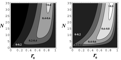
Figure 3: Minimum information gain $G$ versus $r_{0}$ and $N$. Left picture refers to $M=1$, right picture to $M\rightarrow\infty$. (For arbitrary $M$ the scenario is intermediate.) Outside the inconclusive black region we have $G>0$. For $M\rightarrow\infty$ the black region is completely collapsed below $N_{th}=1/2$.

Presence of decoherence. Note that the previous analysis does not consider the presence of thermal noise. Actually this is a good approximation in the optical range, where the number of thermal background photons is around $10^{-26}$ at about $1~{}\mu$m and $300~{}\mathrm{K}$. However, to complete the analysis, we now show that the quantum effect exists even in the presence of stray photons hitting the upper side of the memory and decoherence within the reader. The scattering is modelled as white thermal noise with $\bar{n}$ photons per mode entering each memory cell. Numerically we consider $\bar{n}=10^{-5}$ corresponding to non-trivial diffusion. This scenario may occur when the light, transmitted through the cells, is not readily absorbed by the drive (e.g., using a bucket detector just above the memory) but travels for a while diffusing photons which hit neighboring cells. Assuming the presence of one photon per mode travelling the “optimistic distance” of one meter and undergoing Rayleigh scattering, we get roughly $\bar{n}\simeq 10^{-5}$ Rayleigh . The internal decoherence is modelled as a thermal channel $\mathcal{N}(\varepsilon)$ adding Gaussian noise of variance $\varepsilon$ to each signal/reflected mode, and $2\varepsilon$ to the each idler mode (numerically we consider the non-trivial value $\varepsilon=\bar{n}=10^{-5}$). Now, distinguishing between two reflectivities $\{r_{0},r_{1}\}$ corresponds to discriminating between two Gaussian channels $\mathcal{S}_{u}\otimes\mathcal{N}(2\varepsilon)$ for $u\in\{0,1\}$. Here $\mathcal{S}_{u}:=\mathcal{N}(\varepsilon)\circ\mathcal{E}(r_{u},\bar{n})\circ\mathcal{N}(\varepsilon)$ acts on each signal mode, and contains the attenuator channel $\mathcal{E}(r_{u},\bar{n})$ with conditional loss $r_{u}$ and thermal noise $\bar{n}$. To solve this scenario we use Theorem 1 with the proviso of generalizing the classical discrimination bound. In general, we have $\mathcal{C}=(1-\sqrt{1-F^{M}})/2$, where $F$ is the fidelity between $\mathcal{S}_{0}(|\sqrt{n_{S}}\rangle\langle\sqrt{n_{S}}|)$ and $\mathcal{S}_{1}(|\sqrt{n_{S}}\rangle\langle\sqrt{n_{S}}|)$, the two outputs of a single-mode coherent state $|\sqrt{n_{S}}\rangle$ with $n_{S}:=N/M$ mean photons. Here the expression for $\mathcal{C}$ depends also on the bandwidth $M$ of the classical transmitter $T_{c}=T(M,L,\rho_{c})$. Since $\mathcal{C}$ decreases to zero for $M\rightarrow\infty$, our quantum-classical comparison is now restricted to classical transmitters $T(M,L,\rho_{c})$ with $M$ less than a maximal value $M^{\ast}<\infty$. Remarkably we find that, in the regime of few photons and high reflectivities, narrowband EPR transmitters are able to outperform all the classical transmitters up to an extremely large bandwidth $M^{\ast}$. This is confirmed by the numerical results of Fig. 2, proving the robustness of the quantum effect $G>0$ in the presence of decoherence. Note that we can neglect classical transmitters with extremely large bandwidths (i.e., with $M>M^{\ast}$) since they are not meaningful for the model. In fact, in a practical setting, the signal is an optical pulse with carrier frequency $\nu$ high enough to completely resolve the target cell. This pulse has frequency bandwidth $w\ll\nu$ and duration $\tau\simeq w^{-1}$. Assuming an output detector with response time $\delta t\lesssim\tau$ and “reading time” $t>\tau$, the number of modes which are excited is roughly $M=wt$. In other words, the bandwidth of the signal $M$ is the product of its frequency bandwidth $w$ and the reading time of the detector $t$. Now, the limit $M\rightarrow\infty$ corresponds to $\delta t\rightarrow 0$ (infinite detector resolution) or $t\rightarrow\infty$ (infinite reading time). As a result, transmitters with too large an $M$ can be discarded.

Sub-optimal receiver. The former results are valid assuming optimal output detection. Here we show an explicit receiver design which is (i) easy to construct and (ii) able to approximate the optimal results. This sub-optimal receiver consists of a continuous variable Bell measurement (i.e., a balanced beam-splitter followed by two homodyne detectors) whose output is classically processed by a suitable $\chi^{2}$-test with significance level $\varphi$ (see Appendix for details). In this case the information gain $G$ can be optimized jointly over the signal bandwidth $M$ (i.e., the number of input TMSV states) and the significance level of the output test $\varphi$. As shown in Fig. 4, the advantages of quantum reading are fully preserved.

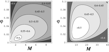
Figure 4: Left. $G$ optimized over $M$ and $\varphi$. $G$ can be higher than $0.6$ bit per cell. Results are shown in the absence of decoherence ($\varepsilon=\bar{n}=0$) considering $r_{0}=0.85$, $r_{1}=1$ and $N=35$. Right. $G$ optimized over $M$ and $\varphi$. Results are shown in the presence of decoherence ($\bar{n}=\varepsilon=10^{-5}$) considering $r_{0}=0.85$, $r_{1}=0.95$, $N=100$ and $M^{\ast}=10^{6}$.

Error correction. In our basic model of memory we store one bit of information per cell. In an alternative model, information is stored in block of cells by using error correcting codes, so that the readout of data is practically flawless. In this configuration, we show that the error correction overhead which is needed by EPR transmitters can be made very small. By contrast, classical transmitters are useless since they may require more than 100 cells for retrieving a single bit of information in the regime of few photons (see Appendix for details).

Conclusion. Quantum reading is able to work in the regime of few photons. What does it imply? Using fewer photons means that we can reduce the reading time of the cell, thus accessing higher data-transfer rates. This is a theoretical prediction that can be checked with a pilot experiment (see Appendix). Alternatively, we can fix the total reading time of the memory while increasing its storage capacity (see Appendix for details). The chance of using few photons leads to another interesting application: the safe readout of photodegradable memories, such as dye-based optical disks or photo-sensitive organic microfilms (e.g., containing confidential information.) Here faint quantum light can retrieve the data safely, whereas classical light could only be destructive. More fundamentally, our results apply to the binary discrimination of attenuator channels.

Acknowledgments. This work was partly supported by a Marie Curie Action of the European Union. The author would like to thank the warm hospitality of the W. M. Keck center for extreme quantum information processing (xQIT) at the Massachusetts Institute of Technology. The author also thanks S. L. Braunstein, S. Lloyd, J. H. Shapiro, A. Aspuru-Guzik, R. Nair, R. Munoz-Tapia, C. Ottaviani, N. Datta, M. Mosheni, J. Oppenheim, C. Weedbrook, C. Lupo, S. Mancini, P. Tombesi, G. Adesso, V. P. Belavkin, S. Weigert, M. Paternostro, and G. Gribakin for comments and discussions.

In this appendix, we start by providing some introductory notions on bosonic systems and Gaussian channels (Sec. I). Then, we explicitly connect our memory model with the basic problem of quantum channel discrimination (Sec. II). This connection is explicitly shown in two paradigmatic cases: the basic “pure-loss model”, where the memory cell is represented by a conditional-loss beam-splitter subject to vacuum noise, and the more general “thermal-loss model”, where thermal noise is added in order to include non-trivial effects of decoherence. In the subsequent sections we consider both these models and we provide the basic tools for making the quantum-classical comparison. In particular, in Sec. III, we provide the fundamental bound for studying classical transmitters, i.e., the “classical discrimination bound”. Then, in the next Sec. IV, we review the mathematical tools for studying EPR transmitters. By using these elements, we compare EPR and classical transmitters in Sec. V, where we explain in detail how to achieve the main results presented in our Letter. In particular, for the pure-loss model, we can provide analytical results: the “threshold energy” and “ideal memory” theorems, which are proven in Sec. VI. Then, in Sec. VII, we show how the advantages of quantum reading persist when the optimal output detection is replaced by an easy-to-implement sub-optimal receiver. This receiver consists of a continuous variable Bell measurement followed by a suitable classical processing (one-tailed $\chi^{2}$-test). In Sec. VIII, we show an alternative model of memory where information is stored in block of cells by means of error correcting codes. Here, we compare the amount of error correction overhead which is needed by EPR and classical transmitters in order to provide a “flawless” readout of logical data. This alternative approach is useful for a future practical implementation of the scheme. Sec. IX recalls standard results in classical error correction. Finally, in Sec. X, we discuss the implications of the few-photon regime, where quantum reading outperforms every classical strategy. Here we give general long-term predictions but also an estimation of the current technological facilities in order to realize a pilot experiment.

I Introduction to bosonic systems

A bosonic system with $n$ modes is a quantum system described by a tensor-product Hilbert space $\mathcal{H}^{\otimes n}$ and a vector of quadrature operators

$$\mathbf{\hat{x}}^{T}:=(\hat{q}_{1},\hat{p}_{1},\ldots,\hat{q}_{n},\hat{p}_{n})~{},$$ (4)

satisfying the commutation relations notationCOMM

$$[\mathbf{\hat{x}},\mathbf{\hat{x}}^{T}]=2i\mathbf{\Omega}~{},$$ (5)

where $\mathbf{\Omega}$ is a symplectic form in $\mathbb{R}^{2n}$, i.e.,

$$\mathbf{\Omega}:=\bigoplus\limits_{i=1}^{n}\left(\begin{array}[c]{cc}0&1\\ -1&0\end{array}\right)~{}.$$ (6)

By definition a quantum state $\rho$ of a bosonic system is called “Gaussian” when its Wigner phase-space representation is Gaussian BraREV ; BraREV2 ; GaussSTATES . In such a case, the state is completely described by the first and second statistical moments. In other words, a Gaussian state $\rho$ of $n$ bosonic modes is characterized by a displacement vector

$$\mathbf{\bar{x}}:=\mathrm{Tr}(\mathbf{\hat{x}}\rho)~{},$$ (7)

and a covariance matrix (CM)

$$\mathbf{V}:=\tfrac{1}{2}\mathrm{Tr}\left(\left\{\mathbf{\hat{x},\hat{x}}^{T}\right\}\rho\right)-\mathbf{\bar{x}\bar{x}}^{T}~{},$$ (8)

where $\{,\}$ denotes the anticommutator notationCOMM . The CM is a $2n\times 2n$ real and symmetric matrix which must satisfy the uncertainty principle SIMONprinc ; Alex

$$\mathbf{V}+i\mathbf{\Omega}\geq 0~{}.$$ (9)

An important example of Gaussian state is the two-mode-squeezed vacuum (TMSV) state for two bosonic modes $\{s,i\}$ (whose number-ket representation is given in the Letter). This state has zero mean ($\mathbf{\bar{x}}=0$) and its CM is given by

$$\mathbf{V}=\left(\begin{array}[c]{cc}(2n_{S}+1)\mathbf{I}&2\sqrt{n_{S}(n_{S}+1)}\mathbf{Z}\\ 2\sqrt{n_{S}(n_{S}+1)}\mathbf{Z}&(2n_{S}+1)\mathbf{I}\end{array}\right)~{},$$ (10)

where $n_{S}\geq 0$ and

$$\mathbf{I}=\left(\begin{array}[c]{cc}1&0\\ 0&1\end{array}\right)~{},~{}\mathbf{Z}=\left(\begin{array}[c]{cc}1&0\\ 0&-1\end{array}\right)~{}.$$ (11)

Here $n_{S}$ represents the mean number of thermal photons which are present in each mode. This number is connected with the “two-mode squeezing parameter” QObook  by the relation

$$n_{S}=\sinh^{2}\xi~{}.$$ (12)

Parameter $\xi$ completely characterizes the state (therefore denoted by $\left|\xi\right\rangle\left\langle\xi\right|$) and quantifies the entanglement between the two modes $s$ and $i$ (being an entanglement monotone for this class of states).

Another important example of Gaussian state is the (multimode) coherent state. For $K$ modes this is given by

$$\left|\boldsymbol{\alpha}\right\rangle\left\langle\boldsymbol{\alpha}\right|=\bigotimes\limits_{i=1}^{K}\left|\alpha_{i}\right\rangle\left\langle\alpha_{i}\right|~{},$$ (13)

where $\boldsymbol{\alpha}:=(\alpha_{1},\cdots,\alpha_{K})$ is a row-vector of amplitudes $\alpha_{i}=(q_{i}+ip_{i})/2$. This state has CM equal to the identity and, therefore, is completely characterized by its displacement vector $\mathbf{\bar{x}}$, which is determined by $\boldsymbol{\alpha}$. Starting from the coherent states, we can characterize all the possible states of a bosonic system by introducing the P-representation. In fact, a generic state $\rho$ of $K$ bosonic modes can be decomposed as

$$\rho=\int d^{2K}\boldsymbol{\alpha~{}}\mathcal{P}(\boldsymbol{\alpha})~{}\left|\boldsymbol{\alpha}\right\rangle\left\langle\boldsymbol{\alpha}\right|~{},$$ (14)

where $\mathcal{P}(\boldsymbol{\alpha})$ is a quasi-probability distribution, i.e., normalized to $1$ but generally non-positive (here we use the compact notation $\int d^{2K}\boldsymbol{\alpha}:=\int d^{2}\alpha_{1}\cdots\int d^{2}\alpha_{K}$). By definition, a bosonic state $\rho$ is called “classical” if $\mathcal{P}(\boldsymbol{\alpha})$ is positive, i.e., $\mathcal{P}$ is a proper probability distribution. By contrast, the state is called “non-classical” when $\mathcal{P}(\boldsymbol{\alpha})$ is non-positive. It is clear that a classical state is separable, since Eq. (14) with $\mathcal{P}$ positive corresponds to a state preparation via local operations and classical communications (LOCCs). The borderline between classical and non-classical states is given by the coherent states, for which $\mathcal{P}$ is a delta function. Note also that the classical states are generally non-Gaussian. In fact, one can have a classical state given by a finite ensemble of coherent states (whose $\mathcal{P}$-representation corresponds to a sum of Dirac-deltas).

In general we use the formalism $T(M,L,\rho)$ to denote a “bipartite transmitter” or, more simply, a “transmitter”. This is a compact notation for characterizing simultaneously a bipartite bosonic system and its state. More specifically, $M$ and $L$, represent the number of modes present in two partitions of the system, called signal (sub)system $S$ and idler (sub)system $I$. Then, given this bipartite system, $\rho$ represents the corresponding global state. This notation is very useful when both system and state are variable. By definition, a “transmitter” $T(M,L,\rho)$ is classical (non-classical) when its state $\rho$ is classical (non-classical), i.e., $T_{c}=T(M,L,\rho_{c})$ and $T_{nc}=T(M,L,\rho_{nc})$. In the comparison between different transmitters, one has to fix some of the parameters of the signal (sub)system $S$. The basic parameters of $S$ are the total number of signal modes $M$ (signal bandwidth) and the mean total number of photons $N$ (signal energy).

I.1 Gaussian channels

A Gaussian channel is a completely positive trace-preserving (CPTP) map

$$\mathcal{E}:\rho\rightarrow\sigma:=\mathcal{E}(\rho)$$ (15)

which transforms Gaussian states into Gaussian states. In particular, a one-mode Gaussian channel (i.e., acting on one-mode bosonic states) can be easily described in terms of the statistical moments $\{\mathbf{\bar{x}},\mathbf{V}\}$. This channel corresponds to the transformation HolevoCAN ; CharacATT ; AlexJens

$$\mathbf{V}\rightarrow\mathbf{KVK}^{T}+\mathbf{N~{},~{}\bar{x}\rightarrow K\bar{x}+d~{},}$$ (16)

where $\mathbf{d}$ is an $\mathbb{R}^{2}$-vector, while $\mathbf{K}$ and $\mathbf{N}$ are $2\times 2$ real matrices, with $\mathbf{N}^{T}=\mathbf{N}\geq 0$ and

$$\det\mathbf{N}\geq\left(\det\mathbf{K}-1\right)^{2}~{}.$$ (17)

Important examples of one-mode Gaussian channels are the following:

(i)

The “attenuator channel” $\mathcal{E}(r,\bar{n})$ with loss $r\in[0,1]$ and thermal noise $\bar{n}\geq 0$. This channel can be represented by a beam splitter with reflectivity $r$ which mixes the input mode with a bath mode prepared in a thermal state with $\bar{n}$ mean photons. This channel implements the transformation of Eq. (16) with

$$\mathbf{K}=\sqrt{r}\mathbf{I}~{},~{}\mathbf{N}=(1-r)(2\bar{n}+1)\mathbf{I}~{},$$ (18)

and $\mathbf{d}=0$. In particular, when the thermal noise $\bar{n}$ is negligible, the attenuator channel $\mathcal{E}(r):=\mathcal{E}(r,0)$ is represented by a beam splitter with reflectivity $r$ and a vacuum bath mode.

(ii)

The thermal channel $\mathcal{N}(\varepsilon)$ adding Gaussian noise with variance $\varepsilon\geq 0$. This channel implements the transformation of Eq. (16) with

$$\mathbf{K}=\mathbf{I}~{},~{}\mathbf{N}=\varepsilon\mathbf{I}~{},$$ (19)

and $\mathbf{d}=0$. This kind of channel is suitable to describe the effects of decoherence when the loss is negligible. This is a typical situation within optical apparatuses which are small in size (as is the case of our memory reader).

It is clear that, for every pair of Gaussian channels, $\mathcal{E}$ and $\mathcal{E}^{\prime}$, acting on the same state space, their composition $\mathcal{E}\circ\mathcal{E}^{\prime}$ is a also Gaussian channel. If $\mathcal{E}$ and $\mathcal{E}^{\prime}$ are Gaussian channels acting on two different spaces, their tensor product $\mathcal{E}\otimes\mathcal{E}^{\prime}$ is also Gaussian. Hereafter we call “bipartite Gaussian channel” a Gaussian channel which is in the tensor-product form $\mathcal{E}\otimes\mathcal{E}^{\prime}$. The action of a bipartite Gaussian channel on a two-mode bosonic state is very simple in terms of its second statistical moments. In fact, let us consider two bosonic modes, $A$ and $B$, in a state $\rho_{AB}$ with generic CM

$$\mathbf{V}=\left(\begin{array}[c]{cc}\mathbf{A}&\mathbf{C}\\ \mathbf{C}^{T}&\mathbf{B}\end{array}\right)~{},$$ (20)

where $\mathbf{A},$ $\mathbf{B}$ and $\mathbf{C}$ are $2\times 2$ real matrices. At the output of a bipartite Gaussian channel $\mathcal{E}^{A\otimes B}:=\mathcal{E}_{A}\otimes\mathcal{E}_{B}$, we have the CM

$$\mathbf{V}_{out}=\left(\begin{array}[c]{cc}\mathbf{K}_{A}\mathbf{AK}_{A}^{T}+\mathbf{N}_{A}&\mathbf{K}_{A}\mathbf{CK}_{B}^{T}\\ \mathbf{K}_{B}\mathbf{C}^{T}\mathbf{K}_{A}^{T}&\mathbf{K}_{B}\mathbf{BK}_{B}^{T}+\mathbf{N}_{B}\end{array}\right)~{},$$ (21)

where the matrices $(\mathbf{K}_{A},\mathbf{N}_{A})$ refer to $\mathcal{E}_{A}$ (acting on the first mode), while $(\mathbf{K}_{B},\mathbf{N}_{B})$ refer to $\mathcal{E}_{B}$ (acting on the second mode).

Proof.  Both the channels $\mathcal{E}_{A}\otimes\mathcal{E}_{B}$ are dilated, so that we have

$$\mathcal{E}^{A\otimes B}(\rho_{AB}) =\mathrm{Tr}_{A^{\prime}B^{\prime}}\left[(U_{A^{\prime}A}\otimes U_{BB^{\prime}})\times\right.$$

$$\left.(\left|0\right\rangle\left\langle 0\right|_{A^{\prime}}\otimes\rho_{AB}\otimes\left|0\right\rangle\left\langle 0\right|_{B^{\prime}})(U_{A^{\prime}A}^{\dagger}\otimes U_{BB^{\prime}}^{\dagger})\right],$$

(22)

where $A^{\prime}$ and $B^{\prime}$ are supplementary sets of bosonic modes prepared in vacua, while $U_{A^{\prime}A}$ and $U_{BB^{\prime}}$ are Gaussian unitaries. According to Eq. (22), the input CM $\mathbf{V}$ is subject to three subsequent operations. First, it must be dilated to $\mathbf{I}_{A^{\prime}}\oplus\mathbf{V}\oplus\mathbf{I}_{B^{\prime}}$, where $\mathbf{I}_{A^{\prime}}$ and $\mathbf{I}_{B^{\prime}}$ are identity matrices of suitable dimensions. Then, it is transformed via congruence by $\mathbf{S}_{A^{\prime}A}\oplus\mathbf{S}_{BB^{\prime}}$, where $\mathbf{S}_{A^{\prime}A}$ and $\mathbf{S}_{B^{\prime}B}$ are the symplectic matrices corresponding to $U_{A^{\prime}A}$ and $U_{BB^{\prime}}$, respectively. Finally, raws and columns corresponding to $A^{\prime}$ and $B^{\prime}$ are elided (trace). By setting

$$\mathbf{S}_{A^{\prime}A}=\left(\begin{array}[c]{cc}\mathbf{a}&\mathbf{c}\\ \mathbf{d}&\mathbf{b}\end{array}\right)~{},~{}\mathbf{S}_{BB^{\prime}}=\left(\begin{array}[c]{cc}\mathbf{e}&\mathbf{g}\\ \mathbf{h}&\mathbf{f}\end{array}\right)~{},$$ (23)

we get

$$\mathbf{V}_{out}=\left(\begin{array}[c]{cc}\mathbf{bAb}^{T}+\mathbf{dd}^{T}&\mathbf{bCe}^{T}\\ \mathbf{eC}^{T}\mathbf{b}^{T}&\mathbf{eBe}^{T}+\mathbf{gg}^{T}\end{array}\right)~{}.$$ (24)

Now, by setting

$$\mathbf{K}_{A}:=\mathbf{b~{}},~{}\mathbf{N}_{A}:=\mathbf{dd}^{T}~{},$$ (25)

and

$$\mathbf{K}_{B}:=\mathbf{e~{}},~{}\mathbf{N}_{B}:=\mathbf{gg}^{T}~{},$$ (26)

we get exactly Eq. (21). $\blacksquare$

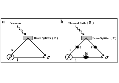
Figure 5: Inset a. Pure-loss model, implementing the bipartite Gaussian channel $\mathcal{G}=\mathcal{E}\otimes\mathcal{I}$. Inset b. Thermal-loss model, implementing the bipartite Gaussian channel $\mathcal{G}=\mathcal{S}\otimes\mathcal{D}$ (see text).

II Memory model and Gaussian channel discrimination

Let us consider the beam-splitter scheme of Fig. 5a, where an input state $\rho$ of two modes (“signal mode” $s$ and “idler mode” $i$) is transformed into an output state $\sigma$. Hereafter we call this scheme the “pure-loss model”. The corresponding transformation is a bipartite Gaussian channel

$$\mathcal{G}=\mathcal{E}(r)\otimes\mathcal{I},$$ (27)

where the attenuator channel $\mathcal{E}(r)$ acts on the signal mode, and the identity channel $\mathcal{I}$ acts on the idler mode. By construction, $\mathcal{G}$ is a memoryless channel. Thus, if we consider a transmitter $T(M,L,\rho)$, i.e., $M$ signal modes $s\in S$ and $L$ idler modes $i\in I$ in a multimode state $\rho$, the input state is transformed into the output state

$$\sigma=\mathcal{G}^{M,L}(\rho)~{},$$ (28)

where

$$\mathcal{G}^{M,L}:=\mathcal{E}(r)^{\otimes M}\otimes\mathcal{I}^{\otimes L}~{}.$$ (29)

This is schematically depicted in Fig. 6.

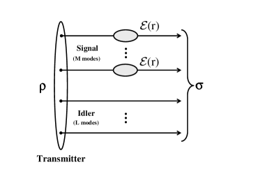
Figure 6: Visual representation of Eq. (29).

Figure 7: Channel discrimination problem (pure-loss model).

Now, encoding a logical bit $u=0,1$ in the reflectivity of the beam splitter $r=r_{u}$ corresponds to encoding the bit into the conditional attenuator channel $\mathcal{E}_{u}:=\mathcal{E}(r_{u})$. Thus, reading a memory cell using an input transmitter $T(M,L,\rho)$, and an output receiver, corresponds to the channel discrimination problem depicted in Fig. 7. The error probability in the decoding of the logical bit, i.e.,

$$P_{err}=\frac{P(u=0|u=1)+P(u=1|u=0)}{2}$$ (30)

corresponds to the error probability of discriminating between the two equiprobable channels $\mathcal{E}_{0}$ and $\mathcal{E}_{1}$. The minimization of this error probability involves the optimization of both input and output. For a fixed input $T(M,L,\rho)$, we have two equiprobable output states, $\sigma_{0}$ and $\sigma_{1}$, with

$$\sigma_{u}=\mathcal{G}_{u}^{M,L}(\rho)=\left(\mathcal{E}_{u}^{\otimes M}\otimes\mathcal{I}^{\otimes L}\right)(\rho)~{}.$$ (31)

The optimal measurement for their discrimination is given by the dichotomic POVM Helstrom

$$E_{0}=\Pi(\gamma_{+})~{},~{}E_{1}=I-\Pi(\gamma_{+})~{},$$ (32)

where $\Pi(\gamma_{+})$ is the projector onto the positive part $\gamma_{+}$ of the Helstrom matrix $\gamma:=\sigma_{0}-\sigma_{1}$ Ppart . Using this measurement, the two output states, $\sigma_{0}$ and $\sigma_{1}$, are discriminated with a minimum error probability which is provided by the Helstrom bound, i.e.,

$$P_{err}(\sigma_{0}\neq\sigma_{1})=\frac{1-D(\sigma_{0},\sigma_{1})}{2}~{},$$ (33)

where $D(\sigma_{0},\sigma_{1})$ is the trace distance between $\sigma_{0}$ and $\sigma_{1}$ Helstrom . In particular,

$$D(\sigma_{0},\sigma_{1}):=\frac{1}{2}\left\|\sigma_{0}-\sigma_{1}\right\|_{1}~{},$$ (34)

where $\left\|\gamma\right\|_{1}:=\mathrm{Tr}\sqrt{\gamma^{\dagger}\gamma}$ is the trace norm. Thus, given two equiprobable channels $\{\mathcal{E}_{0},\mathcal{E}_{1}\}$ and a fixed input transmitter $T$, we can always assume an optimal output detection. Under this assumption (optimal detection), the channel discrimination problem $\mathcal{E}_{0}\neq\mathcal{E}_{1}$ with fixed transmitter $T=T(M,L,\rho)$ is fully characterized by the conditional error probability

$$P_{err}(\mathcal{E}_{0} \neq\mathcal{E}_{1}|T):=\left[\frac{1-D(\sigma_{0},\sigma_{1})}{2}\right]_{\sigma_{u}=\left(\mathcal{E}_{u}^{\otimes M}\otimes\mathcal{I}^{\otimes L}\right)(\rho)}.$$

Now, the minimal error probability for discriminating $\mathcal{E}_{0}$ and $\mathcal{E}_{1}$ is given by optimizing the previous quantity over all the input transmitters, i.e.,

$$P_{err}(\mathcal{E}_{0}\neq\mathcal{E}_{1})=\min_{T}P_{err}(\mathcal{E}_{0}\neq\mathcal{E}_{1}|T)~{}.$$ (36)

In general, this error probability tends to zero in the limit of infinite energy $N\rightarrow+\infty$ (this happens whenever $\mathcal{E}_{0}\neq\mathcal{E}_{1}$). For this reason, in order to consider a non-trivial quantity, we must fix the signal-energy $N$ in the previous minimization. Let us denote by $T|N$ the class of transmitters signalling $N$ photons. Then, we can define the conditional error probability

$$P_{err}(\mathcal{E}_{0}\neq\mathcal{E}_{1}|N)=\min_{T|N}P_{err}(\mathcal{E}_{0}\neq\mathcal{E}_{1}|T)~{}.$$ (37)

It is an open question to find the optimal transmitter within the class $T|N$, i.e., realizing the minimization of Eq. (37). The central idea of our Letter is a direct consequence of this open question. In fact, strictly connected with this question, there is another fundamental problem, whose resolution sensibly narrows the search for optimal transmitters: within the conditional class $T|N$, can we find a non-classical transmitter which outperforms any classical transmitter? More exactly, given two attenuator channels $\{\mathcal{E}_{0},\mathcal{E}_{1}\}$ and fixed signal-energy $N$, can we find any $T_{nc}$ such that

$$P_{err}(\mathcal{E}_{0}\neq\mathcal{E}_{1}|T_{nc})<P_{err}(\mathcal{E}_{0}\neq\mathcal{E}_{1}|T_{c})~{},$$ (38)

for every $T_{c}$? In our Letter we solve this problem Noteshort . In particular, we show this is possible for an important physical regime, i.e., for channels $\{\mathcal{E}_{0},\mathcal{E}_{1}\}$ corresponding to high-reflectivities (as typical of optical memories) and signals with few photons (as typical of entanglement sources).

II.1 Introducing thermal noise

In general, the pure-loss model of Fig. 5a represents a very good description in the optical range if we assume the use of a good reading apparatus. To complete the analysis and show the robustness of the model with respect to decoherence, we also consider the presence of thermal noise, as explicitly stated in the Letter. The noisy scenario is the one depicted in Fig. 5b, that we call the “thermal-loss model”. This corresponds to the bipartite Gaussian channel

$$\mathcal{G}=\mathcal{S}\otimes\mathcal{D},$$ (39)

where

$$\mathcal{S}:=\mathcal{N}(\varepsilon)\circ\mathcal{E}(r,\bar{n})\circ\mathcal{N}(\varepsilon)=\mathcal{S}(r,\bar{n},\varepsilon)$$ (40)

acts on the signal mode, and

$$\mathcal{D}=\mathcal{N}(\varepsilon)\circ\mathcal{N}(\varepsilon)=\mathcal{N}(2\varepsilon)$$ (41)

acts on the idler mode. Exactly as before, $\mathcal{G}$ represents a memoryless channel. As a result, the state $\rho$ of an input transmitter $T(M,L,\rho)$ is transformed into an output state $\sigma=\mathcal{G}^{M,L}(\rho)$, where

$$\mathcal{G}^{M,L}:=\mathcal{S}^{\otimes M}\otimes\mathcal{D}^{\otimes L}~{}.$$ (42)

This transformation is depicted in Fig. 8. Now, encoding a logical bit $u=0,1$ in the reflectivity of the beam splitter $r=r_{u}$ corresponds to encoding the bit into the Gaussian channel $\mathcal{S}_{u}:=\mathcal{S}(r_{u},\bar{n},\varepsilon)$. It follows that the readout of our memory cell corresponds to the channel discrimination problem depicted in Fig. 9.

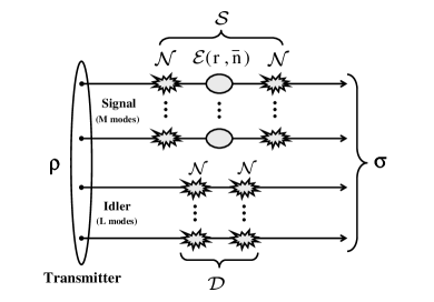
Figure 8: Visual representation of Eq. (42).

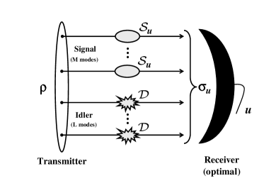
Figure 9: Channel discrimination problem (thermal-loss model).

It is clear that the present thermal scenario (Fig. 9) can be formally achieved by the previous non-thermal one (Fig. 7) via the replacements

$$\mathcal{E}_{u}\rightarrow\mathcal{S}_{u}~{},~{}\mathcal{I}\rightarrow\mathcal{D}~{}.$$ (43)

In this case, the idlers are subject to a non-trivial decoherence channel $\mathcal{D}$, which plays an active role in the discrimination problem. In general, this problem can be formulated as the discrimination of two bipartite channels, $\mathcal{G}_{0}=\mathcal{S}_{0}\otimes\mathcal{D}$ and $\mathcal{G}_{0}=\mathcal{S}_{1}\otimes\mathcal{D}$, using a transmitter $T=T(M,L,\rho)$ and an optimal receiver. The corresponding error probability is defined by

$$P_{err}(\mathcal{G}_{0} \neq\mathcal{G}_{1}|T):=\left[\frac{1-D(\sigma_{0},\sigma_{1})}{2}\right]_{\sigma_{u}=\left(\mathcal{S}_{u}^{\otimes M}\otimes\mathcal{D}^{\otimes L}\right)(\rho)}.$$

Clearly this problem is more difficult to study. For this reason, our basic question becomes the following: given two bipartite channels $\{\mathcal{G}_{0},\mathcal{G}_{1}\}$ and fixed signal-energy $N$, can we find any $T_{nc}$ such that

$$P_{err}(\mathcal{G}_{0}\neq\mathcal{G}_{1}|T_{nc})<P_{err}(\mathcal{G}_{0}\neq\mathcal{G}_{1}|T_{c})~{},$$ (45)

for a suitable large class of $T_{c}$? As stated in the Letter (and explicitly shown afterwards), we can give a positive answer to this question too. This is possible by excluding broadband classical transmitters which are not meaningful for the model (see the Letter for a physical discussion).

In the following Secs. III and IV we introduce the basic tools that we need to compare classical and non-classical transmitters, in both the models: pure-loss and thermal-loss. In particular, Sec. III provides one of the central results of the work: the “classical discrimination bound”, which enables us to bound all the classical transmitters. Then, Sec. IV concerns the study of the non-classical EPR transmitter. At that point we have all the elements to make the comparison, i.e., replying to the questions in Eqs. (38) and (45). This comparison is thoroughly discussed in Sec. V. In particular, for the pure-loss model, we can also derive analytical results, as shown in Sec. VI. These results are the “threshold energy” theorem and the “ideal memory” theorem.

III Classical discrimination bound

III.1 Thermal-loss model

Let us consider the discrimination of two bipartite Gaussian channels

$$\mathcal{G}_{0}=\mathcal{S}_{0}\otimes\mathcal{D}=\mathcal{G}(r_{0},\bar{n},\varepsilon)~{},$$ (46)

and

$$\mathcal{G}_{1}=\mathcal{S}_{1}\otimes\mathcal{D}=\mathcal{G}(r_{1},\bar{n},\varepsilon)~{},$$ (47)

by using a bipartite transmitter $T=T(M,L,\rho)$ which signals $N$ photons. The global input state can be decomposed using the following bipartite $\mathcal{P}$-representation Prepres ; vectNOT

$$\rho=\int d^{2M}\boldsymbol{\alpha}\int d^{2L}\boldsymbol{\beta~{}}\mathcal{P}(\boldsymbol{\alpha},\boldsymbol{\beta})\left|\boldsymbol{\alpha}\right\rangle_{S}\left\langle\boldsymbol{\alpha}\right|\otimes\left|\boldsymbol{\beta}\right\rangle_{I}\left\langle\boldsymbol{\beta}\right|~{},$$ (48)

where $\boldsymbol{\alpha}:=(\alpha_{1},\cdots,\alpha_{M})$ is a vector of amplitudes for the signal $M$-mode coherent-state

$$\left|\boldsymbol{\alpha}\right\rangle_{S}\left\langle\boldsymbol{\alpha}\right|=\bigotimes\limits_{k=1}^{M}\left|\alpha_{k}\right\rangle\left\langle\alpha_{k}\right|~{},$$ (49)

and $\boldsymbol{\beta}:=(\beta_{1},\cdots,\beta_{L})$ is a vector of amplitudes for the idler $L$-mode coherent-state

$$\left|\boldsymbol{\beta}\right\rangle_{I}\left\langle\boldsymbol{\beta}\right|=\bigotimes\limits_{k=1}^{L}\left|\beta_{k}\right\rangle\left\langle\beta_{k}\right|~{}.$$ (50)

The reduced state for the $M$ signal modes is given by

$$\rho_{S}=\int d^{2M}\boldsymbol{\alpha}~{}\mathcal{P}(\boldsymbol{\alpha})~{}\left|\boldsymbol{\alpha}\right\rangle_{S}\left\langle\boldsymbol{\alpha}\right|~{},$$ (51)

where

$$\mathcal{P}(\boldsymbol{\alpha}):=\int d^{2L}\boldsymbol{\beta}~{}\mathcal{P}(\boldsymbol{\alpha},\boldsymbol{\beta})~{}.$$ (52)

The mean total number of photons in the $M$-mode signal system can be written as

$$N=\int d^{2M}\boldsymbol{\alpha}~{}\mathcal{P}(\boldsymbol{\alpha})~{}E~{},$$ (53)

where

$$E:=\sum_{k=1}^{M}\left|\alpha_{k}\right|^{2}~{}.$$ (54)

Now, conditioned on the value of the bit ($u=0$ or $1$), the global output state at the receiver can be written as

$$\sigma_{u}=\int d^{2M}\boldsymbol{\alpha}\int d^{2L}\boldsymbol{\beta}~{}\mathcal{P}(\boldsymbol{\alpha},\boldsymbol{\beta})~{}\sigma_{u}(\boldsymbol{\alpha})\otimes\gamma(\boldsymbol{\beta})~{},$$ (55)

where

$$\sigma_{u}(\boldsymbol{\alpha}):=\mathcal{S}_{u}^{\otimes M}\left(\left|\boldsymbol{\alpha}\right\rangle_{S}\left\langle\boldsymbol{\alpha}\right|\right)=\bigotimes\limits_{k=1}^{M}\mathcal{S}_{u}(\left|\alpha_{k}\right\rangle\left\langle\alpha_{k}\right|)~{},$$ (56)

and

$$\gamma(\boldsymbol{\beta}):=\mathcal{D}^{\otimes L}\left(\left|\boldsymbol{\beta}\right\rangle_{I}\left\langle\boldsymbol{\beta}\right|\right)=\bigotimes\limits_{k=1}^{L}\mathcal{D}(\left|\beta_{k}\right\rangle\left\langle\beta_{k}\right|)~{}.$$ (57)

Assuming an optimal detection of all the output modes (signals and idlers), the error probability in the channel discrimination (i.e., bit decoding) is given by

$$P_{err}(\mathcal{G}_{0}\neq\mathcal{G}_{1}|T)=\frac{1}{2}\left[1-D(\sigma_{0},\sigma_{1})\right]~{},$$ (58)

where $\sigma_{0}$ and $\sigma_{1}$ are specified by Eq. (55) for $u=0,1$.

The study of this error probability can be greatly simplified in the case of classical transmitters. In fact, by assuming a classical transmitter $T_{c}=T(M,L,\rho_{c})$, the $\mathcal{P}$-representation of Eq. (48) is positive. As a consequence, the error probability can be lower-bounded by a quantity which depends on the signal parameters only, i.e.,

$$P_{err}(\mathcal{G}_{0}\neq\mathcal{G}_{1}|T_{c})\geq\mathcal{C}(M,N)~{}.$$ (59)

In other words, for fixed $\mathcal{G}_{0}$ and $\mathcal{G}_{1}$, we can write a lower bound which holds for all the classical transmitters emitting signals with bandwidth $M$ and energy $N$. This is the basic result stated in the following theorem.

Theorem 4

Let us consider the discrimination of two bipartite Gaussian channels, $\mathcal{G}_{0}=\mathcal{S}_{0}\otimes\mathcal{D}=\mathcal{G}(r_{0},\bar{n},\varepsilon)$ and $\mathcal{G}_{1}=\mathcal{S}_{1}\otimes\mathcal{D}=\mathcal{G}(r_{1},\bar{n},\varepsilon)$, by using a classical transmitter $T_{c}=T(M,L,\rho_{c})$ which signals $N$ photons. The corresponding error probability $P_{err}(\mathcal{G}_{0}\neq\mathcal{G}_{1}|T_{c})$ is lower-bounded ($\geq$) by

$$\mathcal{C}(M,N):=\frac{1-\sqrt{1-F(n_{S})^{M}}}{2}~{},$$ (60)

where $F(n_{S})$ is the fidelity between $\mathcal{S}_{0}(|\sqrt{n_{S}}\rangle\langle\sqrt{n_{S}}|)$ and $\mathcal{S}_{1}(|\sqrt{n_{S}}\rangle\langle\sqrt{n_{S}}|)$, the two outputs of a single-mode coherent state $|\sqrt{n_{S}}\rangle$ with $n_{S}:=N/M$ mean photons. In particular, in terms of all the parameters, we have

$$F(n_{S})=\omega^{-1}\exp(-\lambda n_{S})~{},$$ (61)

where $\omega$ and $\lambda$ are defined by

$$\omega:=\frac{1}{2}\left[\xi_{0}\xi_{1}+1-\sqrt{(\xi_{0}^{2}-1)(\xi_{1}^{2}-1)}\right]\geq 1~{},$$ (62)

and

$$\lambda:=\frac{2\left(\sqrt{r_{0}}-\sqrt{r_{1}}\right)^{2}}{\xi_{0}+\xi_{1}}\geq 0~{},$$ (63)

with

$$\xi_{u}:=1+2\bar{n}(1-r_{u})+\varepsilon(1+r_{u})\geq 1~{}.$$ (64)

Proof.  The two possible states, $\sigma_{0}$ and $\sigma_{1}$, describing the whole set of output modes (signals and idlers) are given by Eq. (55), under the assumption that $\mathcal{P}(\boldsymbol{\alpha},\boldsymbol{\beta})$ is positive. In order to lowerbound the error probability

$$P_{err}(\mathcal{G}_{0}\neq\mathcal{G}_{1}|T_{c})=\frac{1}{2}\left[1-D(\sigma_{0},\sigma_{1})\right]~{},$$ (65)

we upperbound the trace distance $D(\sigma_{0},\sigma_{1})$. Since $\mathcal{P}(\boldsymbol{\alpha},\boldsymbol{\beta})$ is a proper probability distribution, we can use the joint convexity of the trace distance NielsenBook . Using this property, together with the stability of the trace distance under addition of systems NielsenBook , we get

$$D(\sigma_{0},\sigma_{1})\leq\int d^{2M}\boldsymbol{\alpha}\int d^{2L}\boldsymbol{\beta~{}}\mathcal{P}(\boldsymbol{\alpha},\boldsymbol{\beta})\times$$

$$D\left[\sigma_{0}(\boldsymbol{\alpha})\otimes\gamma(\boldsymbol{\beta}),\sigma_{1}(\boldsymbol{\alpha})\otimes\gamma(\boldsymbol{\beta})\right]=$$

$$\int d^{2M}\boldsymbol{\alpha}\int d^{2L}\boldsymbol{\beta}~{}\mathcal{P}(\boldsymbol{\alpha},\boldsymbol{\beta})~{}D\left[\sigma_{0}(\boldsymbol{\alpha}),\sigma_{1}(\boldsymbol{\alpha})\right]=$$

$$\int d^{2M}\boldsymbol{\alpha}~{}\mathcal{P}(\boldsymbol{\alpha})~{}D\left[\sigma_{0}(\boldsymbol{\alpha}),\sigma_{1}(\boldsymbol{\alpha})\right]~{},$$ (66)

where $\mathcal{P}(\boldsymbol{\alpha})$ is the marginal distribution defined in Eq. (52). In general, it is known that Fuchs ; FuchsThesis

$$D(\rho,\sigma)\leq\sqrt{1-F(\rho,\sigma)}~{},$$ (67)

for every pair of quantum states $\rho$ and $\sigma$. As a consequence, we can immediately write

$$D\left[\sigma_{0}(\boldsymbol{\alpha}),\sigma_{1}(\boldsymbol{\alpha})\right]\leq\sqrt{1-F[\sigma_{0}(\boldsymbol{\alpha}),\sigma_{1}(\boldsymbol{\alpha})]}~{},$$ (68)

where $F[\sigma_{0}(\boldsymbol{\alpha}),\sigma_{1}(\boldsymbol{\alpha})]$ is the fidelity between the two outputs $\sigma_{0}(\boldsymbol{\alpha})$ and $\sigma_{1}(\boldsymbol{\alpha})$ defined by Eq. (56). Now we can exploit the multiplicativity of the fidelity under tensor products of density operators. In other words, we can decompose

$$F[\sigma_{0}(\boldsymbol{\alpha}),\sigma_{1}(\boldsymbol{\alpha})]=$$

$$F\left[\bigotimes_{k=1}^{M}\mathcal{S}_{0}(\left|\alpha_{k}\right\rangle\left\langle\alpha_{k}\right|),\bigotimes_{k=1}^{M}\mathcal{S}_{1}(\left|\alpha_{k}\right\rangle\left\langle\alpha_{k}\right|)\right]=$$

$$\prod_{k=1}^{M}F\left[\mathcal{S}_{0}(\left|\alpha_{k}\right\rangle\left\langle\alpha_{k}\right|),\mathcal{S}_{1}(\left|\alpha_{k}\right\rangle\left\langle\alpha_{k}\right|)\right]:=\prod_{k=1}^{M}F_{k}~{},$$ (69)

where $F_{k}$ is the fidelity between the two single-mode Gaussian states $\mathcal{S}_{0}(\left|\alpha_{k}\right\rangle\left\langle\alpha_{k}\right|)$ and $\mathcal{S}_{1}(\left|\alpha_{k}\right\rangle\left\langle\alpha_{k}\right|)$. In order to compute $F_{k}$, let us consider the explicit action of $\mathcal{S}_{u}$ on the coherent state $\left|\alpha_{k}\right\rangle\left\langle\alpha_{k}\right|$, which is a Gaussian state with CM $\mathbf{V}=\mathbf{I}$ and displacement $\mathbf{\bar{x}}^{T}=(2$Re$(\alpha_{k}),2$Im$(\alpha_{k}))$. At the output of $\mathcal{S}_{u}$, we get a Gaussian state $\mathcal{S}_{u}(\left|\alpha_{k}\right\rangle\left\langle\alpha_{k}\right|)$ whose statistical moments are proportional to the input ones, i.e., $\mathbf{V}_{u}=\xi_{u}\mathbf{I}$ and $\mathbf{\bar{x}}_{u}=\sqrt{r_{u}}\mathbf{\bar{x}}$, were $\xi_{u}$ is given in Eq. (64). Notice that $\xi_{u}\geq 1$ because $\mathbf{V}_{u}$ must be a bona-fide CM Alex . Then, by using the formula of Ref. FidFormulas , we can compute the analytical expression of the fidelity, which is equal to

$$F_{k}=\omega^{-1}\exp\left[-\lambda\left|\alpha_{k}\right|^{2}\right]~{},$$ (70)

where $\omega$ and $\lambda$ are defined in Eqs. (62) and (63), respectively. It is trivial to check that $\omega\geq 1$ and $\lambda\geq 0$ using $\xi_{u}\geq 1$.  Now, using Eq. (70) into Eq. (69), we get

$$F[\sigma_{0}(\boldsymbol{\alpha}),\sigma_{1}(\boldsymbol{\alpha})]=\omega^{-M}\exp\left[-\lambda\sum_{k=1}^{M}\left|\alpha_{k}\right|^{2}\right]=g(E)~{},$$ (71)

where

$$g(E):=\omega^{-M}\exp\left[-\lambda E\right]~{},$$ (72)

and $E$ is defined in Eq. (54). Thus, by combining Eqs. (66), (68) and (71), we get

$$D(\sigma_{0},\sigma_{1})\leq\mathcal{I}:=\int d^{2M}\boldsymbol{\alpha}~{}\mathcal{P}(\boldsymbol{\alpha})~{}\mathcal{B}(E)~{},$$ (73)

where we have introduced the $\mathbb{R}^{+}\rightarrow[0,1]$ function

$$\mathcal{B}(E):=\sqrt{1-g(E)}~{}.$$ (74)

Since the latter quantity depends only on the real scalar $E$, we can greatly simplify the integral $\mathcal{I}$ in Eq. (73). For this sake, let us introduce the polar coordinates

$$\boldsymbol{\alpha}=\sqrt{\mathbf{e}}\exp(i\boldsymbol{\theta})~{},$$ (75)

where $\mathbf{e}:=(e_{1},\cdots,e_{M})$ is a vector with generic element $e_{k}:=\left|\alpha_{k}\right|^{2}$, and $\boldsymbol{\theta}:=(\theta_{1},\cdots,\theta_{M})$ is a vector of phases (here $d^{2M}\boldsymbol{\alpha}=2^{-M}d^{M}\mathbf{e}d^{M}\boldsymbol{\theta}$). Then, we can write

$$\mathcal{I}=\int_{0}^{+\infty}d^{M}\mathbf{e}~{}\mathcal{R}(\mathbf{e})~{}\mathcal{B}(E)~{},$$ (76)

where $\mathcal{R}(\mathbf{e})$ is the radial probability distribution

$$\mathcal{R}(\mathbf{e}):=\int_{0}^{2\pi}\frac{d^{M}\boldsymbol{\theta}}{2^{M}}~{}\mathcal{P}(\mathbf{e,}\boldsymbol{\theta})~{},$$ (77)

and

$$\mathcal{P}(\mathbf{e,}\boldsymbol{\theta}):=\left[\mathcal{P}(\boldsymbol{\alpha})\right]_{\boldsymbol{\alpha}=\sqrt{\mathbf{e}}\exp(i\boldsymbol{\theta})}~{}.$$ (78)

The integral can be further simplified by setting

$$e_{M}=E-\sum_{k=1}^{M-1}e_{k}~{},$$ (79)

which introduces the further change of variables

$$\mathbf{e}\rightarrow\mathbf{e}^{\prime}:=(e_{1},\cdots,e_{M-1},E)~{}.$$ (80)

Then, we get

$$\mathcal{I}=\int_{0}^{+\infty}dE~{}\mathcal{R}(E)~{}\mathcal{B}(E)~{},$$ (81)

where

$$\mathcal{R}(E) :=\int_{0}^{E}de_{1}\int_{0}^{E-e_{1}}de_{2}\times$$

$$\cdots\times\int_{0}^{E-\sum_{k=1}^{M-2}e_{k}}de_{M-1}~{}\mathcal{R}(\mathbf{e}^{\prime})~{},$$ (82)

and

$$\mathcal{R}(\mathbf{e}^{\prime}):=\left[\mathcal{R}(\mathbf{e})\right]_{e_{M}=E-\sum_{k=1}^{M-1}e_{k}}~{}.$$ (83)

It is clear that the simplification of the integral from Eq. (73) to Eq. (81) can be done not just for $\mathcal{B}(E)$, but for a generic integrable function $f(E)$. As a consequence, we can repeat the same simplification for $f(E)=E$, which corresponds to write the following expression for the mean total number of photons

$$N=\int_{0}^{+\infty}dE~{}\mathcal{R}(E)~{}E~{}.$$ (84)

Analytically, it is easy to check that $\mathcal{B}(E)$ is concave, i.e.,

$$p\mathcal{B}(E)+(1-p)\mathcal{B}(E^{\prime})\leq\mathcal{B}[pE+(1-p)E^{\prime}]~{},$$ (85)

for every $E,E^{\prime}\in\mathbb{R}^{+}$ and $p\in[0,1]$. Then, applying Jensen’s inequality Jensen , we get

$$\mathcal{I} \leq\mathcal{B}\left[\int_{0}^{+\infty}dE~{}\mathcal{R}(E)~{}E\right]=\mathcal{B}\left(N\right)$$

$$=\sqrt{1-g(N)}~{}.$$ (86)

Here we can set

$$g(N)=F(n_{S})^{M}~{},$$ (87)

where $n_{S}=N/M$ and $F(n_{S})$ is given in Eq. (61). According to Eq. (70), $F(n_{S})$ represents the fidelity between the two states $\mathcal{S}_{0}(|\sqrt{n_{S}}\rangle\langle\sqrt{n_{S}}|)$ and $\mathcal{S}_{1}(|\sqrt{n_{S}}\rangle\langle\sqrt{n_{S}}|)$, i.e., the two possible outputs of the coherent state $|\sqrt{n_{S}}\rangle$. In conclusion, by combining Eqs. (73), (86) and (87), we get

$$D(\sigma_{0},\sigma_{1})\leq\sqrt{1-F(n_{S})^{M}}~{}.$$ (88)

Using the latter equation with Eq. (65), we obtain the lower bound of Eq. (60). $\blacksquare$

According to the previous theorem, the classical discrimination bound $\mathcal{C}(M,N)$ can be computed by assuming a coherent-state transmitter which signals $M$ identical coherent states with $n_{S}=N/M$ mean photons each. This transmitter can be denoted by

$$T_{coh}=T(M,0,|\sqrt{n_{S}}\rangle\langle\sqrt{n_{S}}|^{\otimes M})~{},$$ (89)

and is schematically depicted in Fig. 10. Despite the computation of $\mathcal{C}(M,N)$ can be performed in this simple way, we do not know which classical transmitter is actually able to reach, or approach, the lower bound $\mathcal{C}(M,N)$.

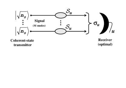
Figure 10: Coherent-state transmitter which signals $M$ copies of a coherent state $|\sqrt{n_{S}}\rangle$ with mean photon number $n_{S}$.

III.2 Pure-loss model

For the pure-loss model of Fig. 7, the previous theorem can be greatly simplified. In particular, we get a classical discrimination bound which does not depend on the bandwidth $M$, but only on the energy $N$ of the signal. This result is stated in the following corollary (which corresponds to the first theorem in our Letter).

Corollary 5

Let us consider the discrimination of two attenuator channels, $\mathcal{E}_{0}=\mathcal{E}(r_{0})$ and $\mathcal{E}_{1}=\mathcal{E}(r_{1})$, by using a classical transmitter $T_{c}=T(M,L,\rho_{c})$ which signals $N$ photons. Then, we have

$$P_{err}(\mathcal{E}_{0}\neq\mathcal{E}_{1}|T_{c})\geq\mathcal{C}(N)~{},$$ (90)

where

$$\mathcal{C}(N):=\frac{1-\sqrt{1-\mathrm{\exp}\left[-N\left(\sqrt{r_{1}}-\sqrt{r_{0}}\right)^{2}\right]}}{2}~{}.$$ (91)

Proof.  Let us set $\bar{n}=\varepsilon=0$ in Theorem 4, so that

$$\mathcal{G}_{u} =\mathcal{S}_{u}\otimes\mathcal{D}=[\mathcal{N}(0)\circ\mathcal{E}(r_{u},0)\circ\mathcal{N}(0)]\otimes[\mathcal{N}(0)\circ\mathcal{N}(0)]$$

$$=[\mathcal{I}\circ\mathcal{E}(r_{u})\circ\mathcal{I}]\otimes[\mathcal{I}\circ\mathcal{I}]=\mathcal{E}_{u}\otimes\mathcal{I}~{}.$$ (92)

Clearly we can write $P_{err}(\mathcal{G}_{0}\neq\mathcal{G}_{1}|T_{c})=P_{err}(\mathcal{E}_{0}\neq\mathcal{E}_{1}|T_{c})$. This quantity is lower-bounded by using Eq. (60) where now the fidelity term $F(n_{S})^{M}$ can be greatly simplified. In fact, because of $\bar{n}=\varepsilon=0$, here we have $\xi_{u}=1$, which implies

$$\omega=1~{},~{}\lambda=\left(\sqrt{r_{0}}-\sqrt{r_{1}}\right)^{2}~{}.$$ (93)

As a consequence, we have

$$F(n_{S})^{M} =\left\{\exp\left[-n_{S}\left(\sqrt{r_{1}}-\sqrt{r_{0}}\right)^{2}\right]\right\}^{M}$$

$$=\exp\left[-N\left(\sqrt{r_{1}}-\sqrt{r_{0}}\right)^{2}\right]~{},$$ (94)

providing the expression of Eq. (91). $\blacksquare$

IV Quantum transmitter

As explained in the Letter, we consider a particular kind of non-classical transmitter, that we call “EPR transmitter”. This is given by

$$T_{epr}=T(M,M,\left|\xi\right\rangle\left\langle\xi\right|^{\otimes M})~{},$$ (95)

where $\left|\xi\right\rangle$ is the TMSV state described in Sec. I. This transmitter is completely characterized by the basic parameters of the emitted signal, i.e., bandwidth $M$ and energy $N$, since $N=Mn_{S}=M\sinh^{2}\xi$. For this reason, we also use the notation $T_{epr}=T_{M,N}$. Given this transmitter, we now show how to compute the error probability which affects the channel discrimination. We consider the general case of the thermal-loss model, but it is understood that the results hold for the pure-loss model by setting $\bar{n}=\varepsilon=0$.

Given an arbitrary EPR transmitter, the corresponding input state

$$\rho=\left|\xi\right\rangle\left\langle\xi\right|^{\otimes M}~{},$$ (96)

is transformed into the conditional output state

$$\sigma_{u}=\varphi_{u}^{\otimes M}~{},$$ (97)

where

$$\varphi_{u}=\mathcal{G}_{u}\left(\left|\xi\right\rangle\left\langle\xi\right|\right)=\left(\mathcal{S}_{u}\otimes\mathcal{D}\right)(\left|\xi\right\rangle\left\langle\xi\right|)~{}.$$ (98)

The single-copy output state $\varphi_{u}$ has zero mean and its CM $\mathbf{V}_{u}$ can be easily computed from the one of the TMSV state, which is given in Eq. (10). In fact, if we write the bipartite channel

$$\mathcal{S}_{u}\otimes\mathcal{D}=[\mathcal{N}(\varepsilon)\circ\mathcal{E}(r_{u},\bar{n})\circ\mathcal{N}(\varepsilon)]\otimes\mathcal{N}(2\varepsilon)$$ (99)

in terms of $(\mathbf{K,N})$ matrices by using Eqs. (18) and (19), we can exploit the result of Eq. (21). Thus, we get the output CM

$$\mathbf{V}_{u}=\left(\begin{array}[c]{cc}[r_{u}(\mu+\varepsilon)+(1-r_{u})\beta+\varepsilon]\mathbf{I}&\sqrt{r_{u}(\mu^{2}-1)}\mathbf{Z}\\ \sqrt{r_{u}(\mu^{2}-1)}\mathbf{Z}&(\mu+2\varepsilon)\mathbf{I}\end{array}\right)~{},$$ (100)

where

$$\mu:=2n_{S}+1~{},~{}\beta:=2\bar{n}+1~{}.$$ (101)

Now, the error probability which affects the channel discrimination $P_{err}(\mathcal{G}_{0}\neq\mathcal{G}_{1}|T_{M,N})$ is equal to the minimum error probability in the M-copy discrimination between $\varphi_{0}$ and $\varphi_{1}$. This quantity is upper-bounded by the quantum Chernoff bound, i.e.,

$$P_{err}(\mathcal{G}_{0}\neq\mathcal{G}_{1}|T_{M,N})\leq\mathcal{Q}(M,N)~{}.$$ (102)

where

$$\mathcal{Q}(M,N)=\frac{1}{2}\left[\inf_{t\in(0,1)}\mathrm{Tr}\left(\varphi_{0}^{t}\varphi_{1}^{1-t}\right)\right]^{M}~{}.$$ (103)

To compute $\mathcal{Q}(M,N)$ we perform the normal-mode decomposition of the Gaussian states $\varphi_{0}$ and $\varphi_{1}$, which corresponds to the symplectic decomposition of the conditional CM of Eq. (100) MinkoPRA ; Alex . Then, we apply the symplectic formula of Ref. MinkoPRA . Unfortunately, the result is extremely long to be presented here (but short analytical expressions are provided afterwards in the proofs for the pure-loss model). Note that an alternative upper-bound is the quantum Battacharyya bound, which is given by

$$\mathcal{B}(M,N)=\frac{1}{2}\left[\mathrm{Tr}\left(\varphi_{0}^{1/2}\varphi_{1}^{1/2}\right)\right]^{M}\geq\mathcal{Q}(M,N)~{}.$$ (104)

This bound is larger but generally easier to compute than the quantum Chernoff bound (see Ref. MinkoPRA for details).

V Quantum-classical comparison

In this section we show how to make the comparison between the EPR transmitter and the classical transmitters in order to reply to the basic questions of Eqs. (38) and (45). Our strategy is to derive a sufficient condition for the superiority of the EPR transmitter by comparing the bounds derived in the previous sections. On the one hand, we know that the error probability of any classical transmitter $P_{err}^{class}$ is lower-bounded by $\mathcal{C}$. On the other hand, the error probability of the EPR transmitter $P_{err}^{epr}$ is upper-bound by $\mathcal{Q}$. Thus, a sufficient condition for $P_{err}^{epr}<P_{err}^{class}$ is provided by the inequality $\mathcal{Q}<\mathcal{C}$. Depending on the model, our answer can be analytical or numerical.

V.1 Pure-loss model

For the pure-loss model, we have $\mathcal{Q}=\mathcal{Q}(M,N)$ and $\mathcal{C}=\mathcal{C}(N)$. Since here the classical discrimination bound is not dependent on the bandwidth, it is sufficient to find a $\bar{M}$ such that $\mathcal{Q}(\bar{M},N)<\mathcal{C}(N)$. In other words, our basic question of Eq. (38) becomes the following: given two channels $\{\mathcal{E}_{0},\mathcal{E}_{1}\}$ and signal-energy $N$, can we find a bandwidth $\bar{M}$ such that

$$\mathcal{Q}(\bar{M},N)<\mathcal{C}(N)~{}?$$ (105)

This clearly implies the existence of an EPR transmitter $T_{\bar{M},N}$ such that

$$P_{err}(\mathcal{E}_{0}\neq\mathcal{E}_{1}|T_{\bar{M},N})<P_{err}(\mathcal{E}_{0}\neq\mathcal{E}_{1}|T_{c})~{},$$ (106)

for every $T_{c}$. As stated in our Letter this question has a positive answer, and this is provided by our “threshold energy” theorem. According to this theorem, for every pair of attenuator channels $\{\mathcal{E}_{0},\mathcal{E}_{1}\}$ and above a threshold energy $N_{th}$, there is an EPR transmitter (with suitable bandwidth $\bar{M}$) which outperforms any classical transmitter. Furthermore, we can prove a stronger result if one of the two channels is just the identity, e.g., we have $\{\mathcal{E}_{0},\mathcal{I}\}$. In this case we have $N_{th}=1/2$ and $\bar{M}$ is a minimum bandwidth, as stated by the “ideal memory” theorem in our Letter. We give the explicit proofs of these theorems in Sec. VI.

In order to quantify numerically the advantage brought by the EPR transmitter, we introduce the minimum information gain

$$G:=1-H(\mathcal{Q})-[1-H(\mathcal{C})]=G(M,N)~{},$$ (107)

where

$$H(x):=-x\log_{2}x-(1-x)\log_{2}(1-x)$$ (108)

is the binary Shannon entropy. Finding a bandwidth $\bar{M}$ such that $G(\bar{M},N)>0$ clearly implies the validity of Eq. (106). In terms of memory readout, this quantity lowerbounds the number of bits per cell which are gained by an EPR transmitter $T_{\bar{M},N}$ over any classical transmitter. By using $G$ one can perform extensive numerical investigations NumG . In particular, one can check that narrowband EPR transmitters (i.e., with low $\bar{M}$) are able to give $G>0$ in the regime of few photons $N$ and high-reflectivities (i.e., $r_{0}$ or $r_{1}$ sufficiently close to $1$). These numerical results are shown and discussed in Fig. 2(left) and Fig. 3 of our Letter.

V.2 Thermal-loss model

For the thermal-loss model, we have $\mathcal{Q}=\mathcal{Q}(M,N)$ and $\mathcal{C}=\mathcal{C}(M,N)$. Here the classical discrimination bound $\mathcal{C}$ depends on the bandwidth $M$ and tends monotonically to zero for $M\rightarrow\infty$. This is evident from the general expression of the fidelity term $F(n_{S})^{M}$ which is present in Eq. (60). In fact, from Eq. (61), we get

$$F(n_{S})^{M}=\omega^{-M}\exp(-\lambda N)~{},$$ (109)

which decreases to zero for $M\rightarrow\infty$ whenever $\omega>1$ (as is generally the case for the thermal-loss model). For this reason, let us fix a maximum bandwidth $M^{\ast}$ and consider the minimum value

$$\inf_{M\in[1,M^{\ast}]}\mathcal{C}(M,N)=\mathcal{C}(M^{\ast},N)~{}.$$ (110)

It is clear that, given two bipartite channels $\{\mathcal{G}_{0},\mathcal{G}_{1}\}$ and signal-energy $N$, we have

$$P_{err}(\mathcal{G}_{0}\neq\mathcal{G}_{1}|T_{c})\geq\mathcal{C}(M^{\ast},N)~{},$$ (111)

for every $T_{c}=T(M,L,\rho_{c})$ with signal-bandwidth $M\leq M^{\ast}$. In other words, using $\mathcal{C}(M^{\ast},N)$ we can bound all the classical transmitters up to the maximum bandwidth $M^{\ast}$. As a result, our basic question of Eq. (45) becomes the following: given two bipartite channels $\{\mathcal{G}_{0},\mathcal{G}_{1}\}$ and signal-energy $N$, can we find an EPR transmitter with suitable bandwidth $\bar{M}$ such that

$$\mathcal{Q}(\bar{M},N)<\mathcal{C}(M^{\ast},N)~{}?$$ (112)

This clearly implies the existence of an EPR transmitter $T_{\bar{M},N}$ such that

$$P_{err}(\mathcal{G}_{0}\neq\mathcal{G}_{1}|T_{\bar{M},N})<P_{err}(\mathcal{G}_{0}\neq\mathcal{G}_{1}|T_{c})~{},$$ (113)

for every $T_{c}=T(M,L,\rho_{c})$ with $M\leq M^{\ast}$. As explicitly discussed in the Letter, this question has a positive answer too, and the value of $M^{\ast}$ can be so high to include all the classical transmitters which are physically meaningful for the memory model. However, despite the previous case, here the answer can only be numerical. In fact, the two bipartite channels $\{\mathcal{G}_{0},\mathcal{G}_{1}\}$ are characterized by four parameters $\{r_{0},r_{1},\bar{n},\varepsilon\}$ and the comparison between transmitters involves further three parameters $\{\bar{M},M^{\ast},N\}$. For this reason, the explicit expression of the minimum information gain now depends on seven parameters, i.e.,

$$G=G(\bar{M},M^{\ast},N,r_{0},r_{1},\bar{n},\varepsilon)~{}.$$ (114)

By performing numerical investigations, one can analyze the positivity of $G$, which clearly implies the condition of Eq. (113). According to Fig. 2(right) of our Letter, we can achieve remarkable positive gains when we compare narrowband EPR transmitters (low $\bar{M}$) with wide sets of classical transmitters (large $M^{\ast}$) in the regime of few photons (low $N$) and high reflectivities ($r_{0}$ or $r_{1}$ close to $1$), and assuming the presence of non-trivial decoherence (e.g., $\varepsilon=\bar{n}=10^{-5}$). See the Letter for physical discussions.

VI Analytical results for the pure-loss model

In this section we provide the detailed proofs of the two theorems relative to the pure-loss model: the “threshold energy” theorem and the “ideal memory” theorem. Given two attenuator channels, $\mathcal{E}_{0}=\mathcal{E}(r_{0})$ and $\mathcal{E}_{1}=\mathcal{E}(r_{1})$, and given the signal-energy $N$, the basic problem is to show the existence of an EPR transmitter $T_{M,N}$ which is able to beat the classical discrimination bound $\mathcal{C}(N)$, and, therefore, all the classical transmitters $T_{c}$. The two theorems provide sufficient conditions for the existence of this quantum transmitter.

VI.1 “Threshold energy” theorem

For the sake of completeness we repeat here the statement of the theorem (this is perfectly equivalent to the statement provided in our Letter).

Theorem 6

Let us consider the discrimination of two attenuator channels, $\mathcal{E}_{0}=\mathcal{E}(r_{0})$ and $\mathcal{E}_{1}=\mathcal{E}(r_{1})$ with $r_{0}\neq r_{1}$, by using transmitters with (finite) signal energy

$$N >N_{th}(r_{0},r_{1}):=\frac{2\ln 2}{2-r_{0}-r_{1}-2\sqrt{(1-r_{0})(1-r_{1})}}~{}.$$

Then, there exists an EPR transmitter $T_{\bar{M},N}$, with suitable bandwidth $\bar{M}$, such that

$$P_{err}(\mathcal{E}_{0}\neq\mathcal{E}_{1}|T_{\bar{M},N})<\mathcal{C}(N)~{}.$$ (116)

Proof.  For simplicity, in this proof we use the shorthand notation $P_{err}(T):=P_{err}(\mathcal{E}_{0}\neq\mathcal{E}_{1}|T)$. According to Corollary 5, the error probability for an arbitrary classical transmitter $T_{c}$ is lower-bounded by the classical discrimination bound, i.e., $P_{err}(T_{c})\geq\mathcal{C}(N)$, where $\mathcal{C}(N)$ is given in Eq. (91). Note that, for every $z\in[0,1]$, we have

$$\frac{1-\sqrt{1-z}}{2}\geq\frac{z}{4}~{}.$$ (117)

As a consequence, we can write

$$\mathcal{C}(N)\geq\frac{e^{-Nx^{2}}}{4}:=\mathcal{\tilde{C}}(N)~{},$$ (118)

where

$$x:=\sqrt{r_{1}}-\sqrt{r_{0}}~{}.$$ (119)

Now let us consider an EPR transmitter $T_{M,N}$. The corresponding error probability $P_{err}(T_{M,N})$ can be upper-bounded via the quantum Battacharyya bound $\mathcal{B}(M,N)$ defined in Eq. (104). This bound can be computed from the conditional CM of Eq. (100) by setting $\bar{n}=\varepsilon=0$ (see Sec. IV and Ref. MinkoPRA ). In this problem, for fixed (finite) energy $N$, the bound $\mathcal{B}(M,N)$ is not monotonic in $M$ (easy to check numerically). However, it is regular in $M$ and its asymptotic limit $\mathcal{B}_{\infty}(N):=\lim_{M\rightarrow+\infty}\mathcal{B}(M,N)$ exists. In particular, the asymptotic Battacharyya bound is equal to

$$\mathcal{B}_{\infty}(N)=\frac{e^{-Nw}}{2}~{},$$ (120)

where $w\in[0,3/2]$ is defined by

$$w:=\frac{r_{0}+r_{1}+2}{2}-2\sqrt{r_{0}r_{1}}-\sqrt{(1-r_{0})(1-r_{1})}~{}.$$ (121)

Clearly we have

$$\inf_{M}P_{err}(T_{M,N})\leq\inf_{M}\mathcal{B}(M,N)\leq\mathcal{B}_{\infty}(N)~{},$$ (122)

which means that $\forall\varepsilon>0$, $\exists\bar{M}\in\mathbb{Z}^{+}$ such that

$$P_{err}(T_{\bar{M},N})<\mathcal{B}_{\infty}(N)+\varepsilon~{}.$$ (123)

In order to prove the result, let us impose the threshold condition

$$\mathcal{B}_{\infty}(N)<\mathcal{\tilde{C}}(N)~{}.$$ (124)

Now, if Eq. (124) is satisfied, then we can always take an $\varepsilon>0$ such that

$$\mathcal{\tilde{C}}(N)=\mathcal{B}_{\infty}(N)+\varepsilon~{}.$$ (125)

Then, because of the proposition of Eq. (123), we have that $\exists\bar{M}\in\mathbb{Z}^{+}$ such that

$$P_{err}(T_{\bar{M},N})<\mathcal{\tilde{C}}(N)\leq\mathcal{C}(N)~{}.$$ (126)

For this reason, the next step is to solve Eq. (124) in order to get a threshold condition on the energy $N$. It is easy to check that, by using Eqs. (118)-(121), the condition of Eq. (124) becomes

$$Nf>1~{},$$ (127)

where

$$f:=\frac{w-x^{2}}{\ln 2}$$

$$=\frac{1}{\ln 2}\left[\frac{(1-r_{0})+(1-r_{1})}{2}-\sqrt{(1-r_{0})(1-r_{1})}\right]~{}.$$ (128)

Since $f$ is proportional to the difference between an arithmetic mean and a geometric mean, we have $f\geq 0$, and $f=0$ if and only if $r_{0}=r_{1}$. Thus, if we exclude the singular case $r_{0}=r_{1}$, we can write

$$N>\frac{1}{f}=N_{th}(r_{0},r_{1})~{}.$$ (129)

In conclusion, if the threshold condition of Eq. (129) is satisfied (where $r_{0}\neq r_{1}$), then there exists a bandwidth $\bar{M}$ such that $P_{err}(T_{\bar{M},N})<\mathcal{C}(N).~{}\blacksquare$

VI.2 “Ideal memory” theorem

Here we prove the ideal memory theorem which refers to the case of ideal memories, i.e., having $r_{0}<r_{1}=1$. This scenario corresponds to discriminating between an attenuator channel $\mathcal{E}(r_{0})$ and the identity channel $\mathcal{I}=\mathcal{E}(1)$. For this reason, the quantum Chernoff bound $\mathcal{Q}(M,N)$ has a simple analytical expression, which turns out to be decreasing in $M$ (for fixed energy $N$). Thanks to this monotony, our result can be proven above a minimum bandwidth $\bar{M}$. In fact, $\mathcal{Q}(M,N)$ decreasing in $M$ implies that $G=1-H[\mathcal{Q}(M,N)]-\{1-H[\mathcal{C}(N)]\}$ is increasing in $M$, so that optimal gains are monotonically reached by broadband EPR transmitters. Note that this was not possible to prove for the previous theorem (see Sec. VI.1) since, in that case, the quantum Battacharyya bound $\mathcal{B}(M,N)$ turned out to be non-monotonic in $M$.

For the sake of completeness we repeat here the statement of the “ideal memory” theorem (this is perfectly equivalent to the statement provided in our Letter).

Theorem 7

Let us consider the discrimination of an attenuator channel $\mathcal{E}_{0}=\mathcal{E}(r_{0})$, with $r_{0}<1$, from the identity channel $\mathcal{I}$, by using transmitters with signal energy

$$N\geq N_{th}:=1/2~{}.$$ (130)

Then, there exists a minimum bandwidth $\bar{M}$ such that, for every EPR transmitter $T_{M,N}$ with $M>\bar{M}$, we have

$$P_{err}(\mathcal{E}_{0}\neq\mathcal{I}|T_{M,N})<\mathcal{C}(N)~{}.$$ (131)

Proof.  Given the discrimination problem $\mathcal{E}_{0}\neq\mathcal{I}$ for fixed signal energy $N$, let us consider an EPR transmitter $T_{M,N}$. Its error probability $P_{err}(T_{M,N})=P_{err}(\mathcal{E}_{0}\neq\mathcal{I}|T_{M,N})$ is upper-bounded by the quantum Chernoff bound $\mathcal{Q}(M,N)$, whose analytical expression is greatly simplified here. In fact, we have

$$\mathcal{Q}(M,N)=\frac{1}{2}\left(1+\frac{N}{M}x\right)^{-2M}~{},$$ (132)

where

$$x=1-\sqrt{r_{0}}\in(0,1]~{}.$$ (133)

This expression can be computed using the procedure sketched in Sec. IV by setting $\bar{n}=\varepsilon=0$ and $r_{1}=1$ in the conditional CM of Eq. (100). For fixed energy $N$, it is very easy to check analytically that $\mathcal{Q}(M,N)$ is decreasing in $M$ (strictly decreasing if we exclude the trivial case $N=0$). Since $\mathcal{Q}$ is bounded ($\mathcal{Q}\in[0,1/2]$) and decreasing in $M$, the broadband limit

$$\mathcal{Q}_{\infty}(N):=\lim_{M\rightarrow+\infty}\mathcal{Q}(M,N)$$ (134)

exists, and clearly coincides with the infimum, i.e.,

$$\mathcal{Q}_{\infty}(N)=\inf_{M}\mathcal{Q}(M,N)~{}.$$ (135)

Explicitly, we compute

$$\mathcal{Q}_{\infty}(N)=\frac{1}{2}\exp(-2Nx)~{}.$$ (136)

By definition of limit, Eqs. (134) and (135) mean that $\forall\varepsilon>0$, $\exists\bar{M}\in\mathbb{Z}^{+}$ such that $\forall M>\bar{M}$

$$\mathcal{Q}_{\infty}(N)\leq\mathcal{Q}(M,N)<\mathcal{Q}_{\infty}(N)+\varepsilon~{}.$$ (137)

Now, since we have $P_{err}(T_{M,N})\leq\mathcal{Q}(M,N)$ for every $M$, it is clear that $\forall\varepsilon>0$, $\exists\bar{M}\in\mathbb{Z}^{+}$ such that $\forall M>\bar{M}$

$$P_{err}(T_{M,N})<\mathcal{Q}_{\infty}(N)+\varepsilon~{}.$$ (138)

In order to prove our result, we impose the threshold condition

$$\mathcal{Q}_{\infty}(N)<\mathcal{C}(N)~{},$$ (139)

where $\mathcal{C}(N)$ is the classical discrimination bound. According to Corollary 5, this is given by

$$\mathcal{C}(N)=\frac{1-\sqrt{1-z}}{2}~{},$$ (140)

where

$$z=\exp(-Nx^{2})~{}.$$ (141)

Now, if Eq. (139) is satisfied, then we can always take an $\varepsilon>0$ such that

$$\mathcal{C}(N)=\mathcal{Q}_{\infty}(N)+\varepsilon~{}.$$ (142)

Then, because of the proposition of Eq. (138), we have that $\exists\bar{M}\in\mathbb{Z}^{+}$ such that $\forall M>\bar{M}$

$$P_{err}(T_{M,N})<\mathcal{C}(N)~{}.$$ (143)

Figure 11: Left. Zero-level function $\bar{y}(x)$ plotted in the finite $(x,y)$-plane. Only for $y<\bar{y}(x)$ we have $g(x,y)>0$. Right. Energy function $\bar{N}(r_{0})$ plotted in the infinite $(r_{0},N)$-plane (here restricted to the sector $0<N\leq 1$). Only for $N>$ $\bar{N}(r_{0})$ we have $g=g(r_{0},N)>0$. Dashed line corresponds to the universal energy threshold $N_{th}=1/2$.

Clearly, the next step is to solve Eq. (139) and get a threshold condition on the energy $N$. After simple Algebra, Eq. (139) can be written as

$$g(x,y)>0~{},$$ (144)

where

$$g(x,y):=y^{x^{2}}+y^{4x}-2y^{2x}~{},$$ (145)

and

$$y:=\exp(-N)\in(0,1)~{}.$$ (146)

Note that, in the definition of $y$, we are excluding the singular points $N=0,+\infty$. The function $g(x,y)$ can be easily analyzed on the plane $(0,1]\times(0,1)$. In particular, its zero-level $g(x,y)=0$ is represented by the continuous function $\bar{y}(x)$ which is plotted in Fig. 11(left). The threshold condition of Eq. (144) is equivalent to

$$y<\bar{y}(x)~{}.$$ (147)

As evident from Fig. 11(left), the function $\bar{y}(x)$ is decreasing in $x\in(0,1]$ with extremal values

$$\lim_{x\rightarrow 0^{+}}\bar{y}(x)=\sup_{x\in(0,1]}\bar{y}(x)=e^{-1/4}~{},$$ (148)

and

$$\lim_{x\rightarrow 1^{-}}\bar{y}(x)=\bar{y}(1)=\min_{x\in(0,1]}\bar{y}(x)=\frac{\sqrt{5}-1}{2}~{}.$$ (149)

Equivalently, by using Eqs. (133) and (146), we can put the threshold condition of Eq. (147) in terms of $r_{0}$ and $N$. In particular, Eq. (147) takes the form

$$N>\bar{N}(r_{0})~{},$$ (150)

where $\bar{N}(r_{0})$ is the decreasing function of $r_{0}\in[0,1)$ which is plotted in Fig. 11(right). This function has extremal values

$$\bar{N}(0)=\max_{r_{0}\in[0,1)}\bar{N}(r_{0})=\ln\frac{2}{\sqrt{5}-1}~{},$$ (151)

and

$$\lim_{r_{0}\rightarrow 1^{-}}\bar{N}(r_{0})=\inf_{r_{0}\in[0,1)}\bar{N}(r_{0})=\frac{1}{4}~{}.$$ (152)

In order to have a criterion which is universal, i.e., $r_{0}$-independent, we can consider the sufficient condition

$$N>\max_{r_{0}\in[0,1)}\bar{N}(r_{0})=\ln\frac{2}{\sqrt{5}-1}\simeq 0.48~{},$$ (153)

which clearly implies Eq. (150). More easily we can consider the slightly-larger condition

$$N\geq N_{th}:=1/2~{}.$$ (154)

In conclusion, for every $r_{0}<r_{1}=1$ and (finite) $N\geq N_{th}:=1/2$, there exists a minimum bandwidth $\bar{M}$ such that $\forall M>\bar{M}$ we have $P_{err}(T_{M,N})<\mathcal{C}(N)$.$~{}\blacksquare$

VII Sub-optimal receiver

In our derivations we have assumed that the output receiver is able to perform an optimal measurement given by the “Helstrom’s POVM” of Eq. (32). Despite this measurement has an extremely simple formula, it is not straightforward to implement it using linear optics and photodetection. This problem has been already considered in Ref. Saikat for the case of quantum illumination, where an ingenious receiver design has been proven to harness quantum illumination advantage. Unfortunately this kind of design cannot be applied directly to our scheme, since quantum reading not only has a different task than quantum illumination but also works in a completely different regime (high reflectivities, low thermal-noise and narrowband signals). Note that the working regime of quantum reading is such that strong correlations survive at the output of the process. For this reason, we can consider simpler receiver designs than the ones for quantum illumination. In fact, here we prove that an output Bell detection followed by a simple classical processing is a sub-optimal receiver able to provide remarkable advantages, i.e., comparable to the Helstrom’s POVM. Since Bell detection is a standard measurement (involving linear optics and photodetection) our reading apparatus can be easily implemented in today’s quantum optics labs.

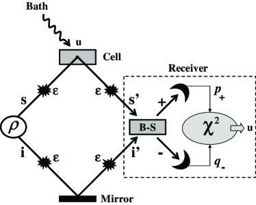
Figure 12: Quantum reading scheme with sub-optimal receiver. This receiver consists of two parts. The first part is a Bell measurement, which consists in a balanced beam-splitter followed by two homodyne detectors. The second part is a classical processing of the outcome $\{q_{-},p_{+}\}$ by means of a $\chi^{2}$-test. See text for more details.

The quantum reading scheme with the sub-optimal receiver is depicted in Fig. 12. The input modes $\{s,i\}$ belong to a TMSV state $\rho=\left|\xi\right\rangle\left\langle\xi\right|$. These modes are processed as usual, i.e., the signal mode $s$ is conditionally transformed by the cell (reflectivity $r_{u}$ encoding the bit $u$) while the idler mode $i$ is sent directly to the receiver. Their quadratures, $\mathbf{\hat{x}}_{s}=(\hat{q}_{s},\hat{p}_{s})^{T}$ and $\mathbf{\hat{x}}_{i}=(\hat{q}_{i},\hat{p}_{i})^{T}$, are transformed according to the input-output relations

$$\mathbf{\hat{x}}_{s}\rightarrow\mathbf{\hat{x}}_{s^{\prime}}=\sqrt{r_{u}}(\mathbf{\hat{x}}_{s}+\mathbf{\hat{x}}_{\varepsilon})+\sqrt{1-r_{u}}\mathbf{\hat{x}}_{b}+\mathbf{\hat{x}}_{\varepsilon}^{\prime}~{},$$ (155)

and

$$\mathbf{\hat{x}}_{i}\rightarrow\mathbf{\hat{x}}_{i^{\prime}}=\mathbf{\hat{x}}_{i}+2\mathbf{\hat{x}}_{\varepsilon}^{\prime\prime}~{},$$ (156)

where $\mathbf{\hat{x}}_{b}$ are the quadratures of the external thermal bath, while $\mathbf{\hat{x}}_{\varepsilon}$, $\mathbf{\hat{x}}_{\varepsilon}^{\prime}$ and $\mathbf{\hat{x}}_{\varepsilon}^{\prime\prime}$ are quadratures associated with the internal thermal channels. At the receiver the two modes $\{s^{\prime},i^{\prime}\}$ are combined in a balanced beam-splitter which outputs the modes $\{-,+\}$ with quadratures

$$\mathbf{\hat{x}}_{-}:=\left(\begin{array}[c]{c}\hat{q}_{-}\\ \hat{p}_{-}\end{array}\right)=\frac{\mathbf{\hat{x}}_{s^{\prime}}-\mathbf{\hat{x}}_{i^{\prime}}}{\sqrt{2}}~{},$$ (157)

and

$$\mathbf{\hat{x}}_{+}:=\left(\begin{array}[c]{c}\hat{q}_{+}\\ \hat{p}_{+}\end{array}\right)=\frac{\mathbf{\hat{x}}_{s^{\prime}}+\mathbf{\hat{x}}_{i^{\prime}}}{\sqrt{2}}~{}.$$ (158)

Here the “EPR quadratures” $\{\hat{q}_{-},\hat{p}_{+}\}$ are measured by using two homodyne detectors. The corresponding outcome $\{q_{-},p_{+}\}$ is classically processed via a $\chi^{2}$-test, whose output is the value of the bit stored in the memory cell. In general, for arbitrary bandwidth $M\geq 1$, we have $M$ identical copies $\left|\xi\right\rangle\left\langle\xi\right|^{\otimes M}$ at the input and, therefore, $2M$ output variables $\{q_{-},p_{+}\}^{M}$ which are processed by the $\chi^{2}$-test.

Let us analyze the detection process in detail in order to derive the error-probability which affects the decoding. First of all we can easily verify that the two classical outputs, $q_{-}$ and $p_{+}$, are identical Gaussian variables, so that we can simply use $z$ to denote $q_{-}$ or $p_{+}$. Clearly the Gaussian variable $z$ is tested two times for each single-copy state $\left|\xi\right\rangle\left\langle\xi\right|$ and, therefore, $2M$ times during the reading time of the logical bit. This variable has zero mean and variance $V=V(u)$ which is conditioned to the value of the stored bit $u=0,1$. Explicitly, we have

$$V(u) =\frac{1}{2}\left[r_{u}(\mu+\varepsilon)+(1-r_{u})\beta+\right.$$

$$\left.\mu+3\varepsilon-2\sqrt{r_{u}(\mu^{2}-1)}\right]~{},$$ (159)

where $r_{u}$ is the conditional reflectivity of the cell, $\mu:=2n_{S}+1$ is the variance associated with the signal-mode, $\beta:=2\bar{n}+1$ is the noise-variance of the external thermal bath, and $\varepsilon$ is the noise-variance of the internal thermal channel. It is clear that the decoding of the logical bit $u$ corresponds to the statistical discrimination between two variances $V(0)$ and $V(1)$. In other words, the variable $z$ is subject to the hypothesis test

$$\left\{\begin{array}[c]{c}\mathrm{H}_{0}~{}(u=0)~{}:~{}V=V(0)~{},\\ \\ \mathrm{H}_{1}~{}(u=1)~{}:~{}V=V(1)~{}.\end{array}\right.$$ (160)

It is easy to show that $V$ of Eq. (159) is a decreasing function of the reflectivity $r_{u}$ as long as

$$r_{u}<\frac{\mu^{2}-1}{(\varepsilon-\beta+\mu)^{2}}~{},$$ (161)

which is always true in the regime considered here (i.e., $\varepsilon$ small and $\beta$ close to $1$). This means that $r_{0}<r_{1}$ implies $V(0)>V(1)$, which makes Eq. (160) a one-tailed test. Equivalently, we can introduce the normalized variable

$$z^{\prime}:=\frac{z}{\sqrt{V(1)}}~{},$$ (162)

with zero mean and variance $V^{\prime}(u)=V(u)/V(1)$, and replace Eq. (160) with the one-tailed test

$$\left\{\begin{array}[c]{c}\mathrm{H}_{0}~{}:~{}V^{\prime}=1+\Sigma~{},\\ \\ \mathrm{H}_{1}~{}:~{}V^{\prime}=1~{}.{}{}{}{}{}{}\end{array}\right.$$ (163)

where

$$\Sigma:=\frac{V(0)-V(1)}{V(1)}>0~{}.$$ (164)

Thus, assuming $r_{0}<r_{1}$, the decoding of the logical bit is equivalent to the statistical discrimination between the two hypotheses in Eq. (163), i.e., $V^{\prime}>1$ and $V^{\prime}=1$. For arbitrary bandwidth $M$, we collect $2M$ independent outcomes $\{z_{1},\cdots z_{2M}\}$ and we construct the $\chi^{2}$-variable

$$\theta:=\sum_{k=1}^{2M}(z_{k}^{\prime})^{2}~{}.$$ (165)

Then, we select one of the two hypotheses according to the following rule

$$\left\{\begin{array}[c]{c}\text{Accept }\mathrm{H}_{0}~{}\Leftrightarrow~{}\theta\geq\mathcal{Q}_{1-\varphi}^{2M-1}~{},\\ \\ \text{Accept }\mathrm{H}_{1}~{}\Leftrightarrow~{}\theta<\mathcal{Q}_{1-\varphi}^{2M-1}~{}.\end{array}\right.$$ (166)

where $\mathcal{Q}_{1-\varphi}^{2M-1}$ is the $(1-\varphi)^{th}$ quantile of the $\chi^{2}$ distribution with $2M-1$ degrees of freedom. Here the quantity $\varphi$ represents the significance level of the test, corresponding to the asymptotic probability of wrongly rejecting the hypothesis $\mathrm{H}_{1}$, i.e.,

$$\varphi=\lim_{M\rightarrow\infty}P(\mathrm{H}_{0}|\mathrm{H}_{1})~{}.$$ (167)

This quantity must be fixed and its value characterizes the test. In particular, for finite $M$, there will be an optimal value of $\varphi$ which maximizes the performance of the test.

Let us explicitly compute the error probability affecting the classical test. For arbitrary variance $V^{\prime}$, the $\chi^{2}$ distribution with $2M-1$ degrees of freedom is equal to

$$P_{M,V^{\prime}}(\theta)=\frac{\theta^{M-1}\exp\left(-\frac{\theta}{2V^{\prime}}\right)}{(2V^{\prime})^{M}\Gamma\left(M\right)}~{},$$ (168)

where $\Gamma(x)$ is the Gamma function. The probability of finding $\theta$ bigger than $t$ is given by the integral

$$I\left(M,V^{\prime},t\right):=\int_{t}^{+\infty}P_{M,V^{\prime}}(\theta)d\theta=\frac{\Gamma\left(M,\frac{t}{2V^{\prime}}\right)}{\Gamma\left(M\right)}~{}.$$ (169)

where $\Gamma\left(x,y\right)$ is the incomplete Gamma function. Thus, given $\mathrm{H}_{1}$ (i.e., $V^{\prime}=1$) the probability of accepting $\mathrm{H}_{0}$ (i.e., $\theta\geq\mathcal{Q}_{1-\varphi}^{2M-1}$) is given by

$$P(\mathrm{H}_{0}|\mathrm{H}_{1})=I\left(M,1,\mathcal{Q}_{1-\varphi}^{2M-1}\right)~{}.$$ (170)

By contrast, given $\mathrm{H}_{0}$ (i.e., $V^{\prime}=1+\Sigma$) the probability of accepting $\mathrm{H}_{1}$ (i.e., $\theta<\mathcal{Q}_{1-\varphi}^{2M-1}$) is given by

$$P(\mathrm{H}_{1}|\mathrm{H}_{0})=1-I\left(M,1+\Sigma,\mathcal{Q}_{1-\varphi}^{2M-1}\right)~{}.$$ (171)

From Eqs. (170) and (171) we compute the error probability affecting the test, which is given by

$$P_{test}:=\frac{1}{2}\left[P(\mathrm{H}_{0}|\mathrm{H}_{1})+P(\mathrm{H}_{1}|\mathrm{H}_{0})\right]$$

$$=\frac{1}{2}+\frac{1}{2}\left[I\left(M,1,\mathcal{Q}_{1-\varphi}^{2M-1}\right)-I\left(M,1+\Sigma,\mathcal{Q}_{1-\varphi}^{2M-1}\right)\right]$$

$$=P_{test}\left(r_{0},r_{1},N,M,\bar{n},\varepsilon,\varphi\right)~{}.$$ (172)

Clearly this quantity depends on all the parameters of the model, i.e., memory reflectivities $\{r_{0},r_{1}\}$, energy and bandwidth of the signal $\{N,M\}$, levels of noise $\{\bar{n},\varepsilon\}$ and significance level of the test $\varphi$. This error probability must be compared with the classical discrimination bound $\mathcal{C}$. For simplicity let us first consider the pure-loss model ($\bar{n}=\varepsilon=0$). In this case $P_{test}=P_{test}\left(r_{0},r_{1},N,M,\varphi\right)$ must be compared with $\mathcal{C}=\mathcal{C}\left(r_{0},r_{1},N\right)$ of Eq. (91). Then, for given memory $\{r_{0},r_{1}\}$ and signal-energy $N$, we have that quantum reading is superior if we find a bandwidth $M$ and a significance level $\varphi$ such that $P_{test}<\mathcal{C}$. This is equivalent to prove the positivity of the (sub-optimal) information gain

$$G_{test}=1-H(P_{test})-[1-H(\mathcal{C})]~{},$$ (173)

which provides a lowerbound to the number of bits per cell which are gained by quantum reading over any classical strategy. In Fig. 13(left) we optimize $G_{test}$ over $M$ and $\varphi$ for an ideal memory in the few-photon regime. Remarkably, we can find an area where $G_{test}>0.6$ bits per cell.

Figure 13: (This is a repetition of Fig. 4). Left. Information gain $G_{test}$ optimized over the bandwidth $M$ (i.e., number of TMSV states) and the significance level of the test $\varphi$. The gain can be higher than $0.6$ bits per cell. The results are shown for the pure-loss model ($\varepsilon=\bar{n}=0$) considering $r_{0}=0.85$, $r_{1}=1$ and $N=35$. Right. Information gain $G_{test}$ optimized over $M$ and $\varphi$. The results are shown for the thermal-loss model ($\bar{n}=\varepsilon=10^{-5}$) considering $r_{0}=0.85$, $r_{1}=0.95$, $N=100$ and $M^{\ast}=10^{6}$.

Then, let us consider the thermal-loss model, with $\bar{n}=\varepsilon=10^{-5}$. In this case, $P_{test}=P_{test}\left(r_{0},r_{1},N,M,\bar{n},\varepsilon,\varphi\right)$ must be compared with $\mathcal{C}=\mathcal{C}\left(r_{0},r_{1},N,M^{\ast},\bar{n},\varepsilon\right)$ where the value of $M^{\ast}$ is high enough to include all the classical transmitters which are meaningful for the model (here we take $M^{\ast}=10^{6}$). In Fig. 13(right), we consider a memory with $r_{0}=0.85$ and $r_{1}=0.95$ (high-reflectivity regime), which is illuminated by a signal with $N=100$ (few-photon regime). The numerical optimization over $M$ and $\varphi$ shows an area where $G_{test}>0.5$ bits per cell.

Thus, the remarkable advantages of quantum reading are still evident when the optimal Helstrom’s POVM is replaced by a sub-optimal receiver, consisting of a Bell measurement followed by a suitable classical post-processing. This sub-optimal receiver can be easily realized in today’s quantum optics labs, thus making quantum reading a technique within the catch of current technology.

VIII Memory Model with Error Correction

In our study, we have considered a theoretical model of memory where each cell stores exactly one bit of information. Then, by fixing the mean total number of photons which are irradiated over each memory cell, we have computed the average information which is retrieved by an input transmitter $T$ and an optimal output detection. This quantity ranges from zero to one and can be written as $I(T):=1-H(P_{err})$, were $P_{err}$ is the error-probability corresponding to $T$. In this scenario, we have compared the information which is retrieved by a non-classical EPR transmitter, lower-bounded by $I_{epr}:=1-H(Q)$, with the information retrieved by an arbitrary classical transmitter, upper-bounded by $I_{c}:=1-H(C)$. This comparison has been quantified by the gain of information $G=I_{epr}-I_{c}$ introduced in Eq. (107). In doing this comparison, we have also considered the presence of thermal noise and the practical case of a sub-optimal receiver, which implies a weaker gain of information as quantified by Eq. (173). Remarkably, we have found regimes (few photons and high reflectivities) where $G$ is strictly positive and can be even close to $1$, meaning that $I_{epr}\simeq 1$ (i.e., an EPR transmitter reads all the information) while $I_{c}\simeq 0$ (i.e., no information can be read by any classical transmitter).

Now it is important to note that our comparison can also be stated in another equivalent way. Instead of storing one bit per cell and evaluating the information read by a transmitter $T$, we can store a logical bit in a block of $m$ cells by using a classical error correcting (EC) code and calculate the minimum $m$ which is needed for a flawless readout by $T$. Then, we compare the block sizes, $m_{epr}$ and $m_{c}$, which are allowed by an EPR transmitter and an optimal classical transmitter. In this scenario, the positivity condition $G>0$ corresponds to $m_{epr}<m_{c}$, meaning that an EPR transmitter involves less overhead of error correction. In particular, for $G\rightarrow 1$ we have $m_{epr}\rightarrow 1$ and $m_{c}\rightarrow\infty$. This corresponds to having negligible overhead for an EPR transmitter versus infinite overhead for any classical transmitter. In this model, the reading time of a logical bit is clearly proportional to the block size $m$. As a result, $m\rightarrow\infty$ corresponds to infinite reading time, i.e., the impossibility to read information. Equivalently, if we fix the total data-size of the memory, its logical capacity is inversely proportional to the block-size $m$. Then, $m\rightarrow\infty$ corresponds to zero logical capacity.

Despite theoretically equivalent, this alternative approach is interesting for practical implementations. In fact, actual digital memories are written using EC codes. As an example, today’s CDs are written using Reed-Solomon codes, which are responsible for an error-correction overhead that is around the 15-20% of the total data DVDbook . In the remainder of the section, we discuss in more detail the memory model based on error-correction, by showing explicit cases where $m_{epr}$ is low while $m_{c}\gg 1$. We start by considering repetition codes since they can easily provide the order of magnitude of the ratio $m_{c}/m_{epr}$. Then, we refine our derivation by considering optimal EC codes, for which we exploit both the Hamming HammREF and Gilbert-Varshamov bounds GilbertREF ; VarshaREF .

VIII.1 Repetition Codes

Let us store a logical bit $\bar{u}$ in a block of $m$ cells by using an $m$-bit repetition code, where $m=2t+1$ is an odd number ($t=0,1,...$) This means that the logical bit $\bar{u}=\bar{0},\bar{1}$ is encoded in $m$ physical bits $u_{1}u_{2}\cdots u_{m}$ via the codewords

$$\bar{0}=\underbrace{00\cdots 0}_{m},\quad\bar{1}=\underbrace{11\cdots 1}_{m}.$$ (174)

Each physical bit $u_{i}$ is stored in a corresponding cell (see Fig. 14). Each cell of the block is sequentially read by an input transmitter $T=T(M,L,\rho)$, signalling $N$ photons, and an optimal output detector. The value of each physical bit $u_{i}$ is retrieved up to an error probability $P_{err}$ which depends on the specific transmitter $T$. After reading all the cells of the block, the output codeword $u_{1}^{\prime}u_{2}^{\prime}\cdots u_{m}^{\prime}$ is corrected by majority voting (see Fig. 14).

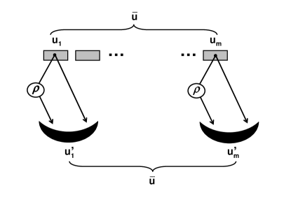
Figure 14: Model of memory with classical error correction (repetition codes). A logical bit $\bar{u}$ is encoded in a block of $m$ cells by using the codeword $u_{1}u_{2}\cdots u_{m}$ of a repetition code. Each cell of the block is sequentially read by a transmitter $T(M,L,\rho)$ and an optimal output detector. After the whole block is read, the output noisy codeword $u_{1}^{\prime}u_{2}^{\prime}\cdots u_{m}^{\prime}$ is corrected by majority voting to provide the encoded bit $\bar{u}$ up a logical error probability $\bar{p}(m,P_{err})$.

Depending on the number of bit-flips, error recovery may fail or not. Up to $t=(m-1)/2$ bit-flips are correctable, while more than $t$ bit-flips leads to a logical error. As a result, the input logical bit $\bar{u}$ is retrieved up to a logical error probability

$$\bar{p}(m,P_{err})=\sum_{i=\frac{m+1}{2}}^{m}\left(\begin{array}[c]{c}m\\ i\end{array}\right)(P_{err})^{i}(1-P_{err})^{m-i}~{}.$$ (175)

By definition, we say that the readout is “flawless” if $\bar{p}(m,P_{err})\leq\varepsilon$ for some small cut-off $\varepsilon$. The value of $\varepsilon$ depends on the size of the memory and the error tolerance that we allow. For instance, for memories of $1$ Gbit, the value $\varepsilon=10^{-9}$ corresponds to having less than $1$ bit of logical data corrupted. Given a transmitter $T$ (and therefore an error probability $P_{err}$), the resolution of the equation $\bar{p}(m,P_{err})=10^{-9}$ identifies a corresponding size $m^{\ast}$ for the encoding block. Clearly, the best transmitter is the one who minimizes the value of $m^{\ast}$. Thus, for fixed signal-energy $N$, we compare the block-sizes of EPR and classical transmitters. Given an EPR transmitter $T_{M,N}$, with bandwidth $M$ and energy $N$, we use the bound $P_{err}\leq\mathcal{Q}(M,N)$ of Eq. (102) to over-estimate the corresponding block-size $m_{epr}^{\ast}$ (upper-bound). Then, for every classical transmitter $T_{c}$ irradiating $N$ photons, we use the bound $P_{err}\geq\mathcal{C}(N)$ of Eq. (90) to under-estimate $m_{c}^{\ast}$ (lower-bound) NOTA1 . It is clear that $m_{epr}^{\ast}<m_{c}^{\ast}$ provides a sufficient condition for the superiority of quantum reading. In particular, we can easily find configurations where $m_{epr}^{\ast}$ is of the order of units while $m_{c}^{\ast}\gg 1$. As a numerical example, let us consider an ideal memory with $r_{0}=0.95$ and $r_{1}=1$, where each cell is irradiated by $N=100$ photons. From Fig. 15, we can see that $m_{epr}^{\ast}$ is decreasing in $M$. In particular, we have $m_{epr}^{\ast}\lesssim 9$ already for small values of $M$, i.e., narrowband EPR transmitters. This numerical result shows that using EPR transmitters we can perfectly read data up to a limited error-correction overhead (as we will show afterwards this overhead can be reduced by using more efficient EC codes).

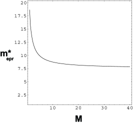
Figure 15: Quantum upper-bound $m_{epr}^{\ast}$ versus the bandwidth $M$ of the EPR transmitter. Other parameters are $r_{0}=0.95$, $r_{1}=1$ and $N=100$. The curve represents an upper-bound for the size of the encoding block which enables an EPR transmitter $T_{M,N}$ to retrieve logical data without errors (i.e., up to a cut-off $\varepsilon=10^{-9}$).

Under the same conditions, the classical lower-bound is extremely high, since we have $m_{c}^{\ast}\approx 560$. In other words, classical transmitters need a huge overhead of error correction, which is more than $60$ times the one needed by EPR transmitters. This clearly makes classical transmitters useless in the present configuration. Similar results can be numerically found with other choices of parameters in the regime of few-photons and high-reflectivities. In the following section we study the model by using optimal EC codes instead of repetition codes. In this more refined derivation, we will see that the EC overhead for classical transmitters is more than $80$ times the one needed by EPR transmitters.

VIII.2 Optimal Error Correcting Codes

The previous derivation based on repetition codes can be generalized to more powerful EC codes. In fact, a more general model of memory consists of encoding $k\geq 1$ logical bits in a block of $m$ cells by using an arbitrary EC code $[m,k,d]$ with distance. This EC code is able to correct up to $t=\lfloor\frac{d-1}{2}\rfloor$ bit-flips, where $\lfloor x\rfloor$ represents the floor function (i.e., the largest integer not greater than $x$). In other words, it corrects up to $(d-1)/2$ bit-flips for odd $d$, and up to $(d/2)-1$ bit-flips for even $d$. By definition, we call $R=k/m$ the rate of the code and $\delta=d/m$ its relative distance. In our memory we fix the size of the block to be very large, e.g., $m=2000$, which is comparable to the size of the data-blocks in current CDs and DVDs. Then, we determine the value of the relative distance $\delta$ which allows a flawless readout of the memory (up to a cut-off $\varepsilon$). Given this value, we choose an EC code which optimizes the rate $R$. The optimal value of $R$ falls in the following range

$$\underline{R}:=1-H(\delta)\leq R\leq 1-H(\delta/2):=\overline{R}~{},$$ (176)

where $H$ is the binary Shannon entropy, i.e.,

$$H(x):=-x\log_{2}x-(1-x)\log_{2}(1-x)~{}.$$ (177)

The inequality of Eq. (176) comes from combining the Hamming (upper)bound and the Gilbert-Varshamov (lower)bound, that we report in Sec. IX for the sake of completeness.

In our quantum-classical comparison, we fix the signal-energy $N$ irradiated over each cell. Then, we compare the optimal rate $R_{epr}$ which is achievable by using an EPR transmitter $T_{M,N}$ with the optimal rate $R_{c}$ achievable by classical transmitters $T_{c}$. More exactly, we compare the quantum lower-bound $\underline{R}_{epr}$ with the classical upper-bound $\overline{R}_{c}$, since $\underline{R}_{epr}>\overline{R}_{c}$ implies $R_{epr}>R_{c}$. In particular, we can show configurations where $\underline{R}_{epr}$ is close to one while $\overline{R}_{c}$ is close to zero. This means that EPR transmitters need a minimal error correction overhead for retrieving the data perfectly. By contrast, classical transmitters need an overhead which is unfeasible for practical implementations. In the following we discuss the quantum-classical comparison in more detail.

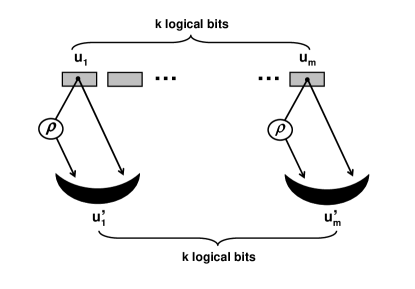
Figure 16: Model of memory with classical error correction (optimal EC codes). By using an optimal EC code $[m,k,d]$ we encode $k$ logical bits in a large block of $m$ cells. Each cell of the block is sequentially read by a transmitter $T(M,L,\rho)$ and an optimal output detector. After the whole block is read, the output noisy codeword $u_{1}^{\prime}u_{2}^{\prime}\cdots u_{m}^{\prime}$ is corrected by standard procedures of syndrome detection and error recovery. The final outcome provides the encoded $k$ logical bits up an error probability $\bar{p}(d,m,P_{err})$.

Let us consider a memory which is subdivided in large blocks, each one composed of $m=2000$ cells. In each block the information is stored by using an optimal EC code $[m,k,d]$ where $k$ and $d$ are to be determined or, equivalently, their relative quantities $R=k/m$ and $\delta=d/m$. For a given a transmitter $T$, we have a corresponding error probability $P_{err}$ affecting the readout of every single cell. After all the cells of one block are read, the output codeword is processed using standard procedures of syndrome detection and error recovery (see Fig. 16). The probability of an uncorrectable error (which causes the lost of $k$ logical bits) corresponds to the probability of having more than $t=\lfloor\frac{d-1}{2}\rfloor$ bit-flips in the block. This quantity is given by NOTA2

$$\bar{p}(d,m,P_{err})=\sum_{i=\lfloor\frac{d+1}{2}\rfloor}^{m}\left(\begin{array}[c]{c}m\\ i\end{array}\right)(P_{err})^{i}(1-P_{err})^{m-i}~{}.$$ (178)

As usual we say that the readout is “flawless” if $\bar{p}(d,m,P_{err})\leq\varepsilon$ for some small cut-off $\varepsilon$, that we set equal to $10^{-9}$ as before. Now for fixed block-size $m=2000$ and cut-off $\varepsilon=10^{-9}$, the resolution of the equation $\bar{p}(d,m,P_{err})=\varepsilon$ provides the distance $d$ as a function of $P_{err}$. Thus, given a transmitter $T$, i.e., an error probability $P_{err}$, we have a corresponding minimum distance $d^{\ast}$ for the code. Once that $d^{\ast}$ is determined, we consider the maximum number of logical bits $k^{\ast}$ which can be stored by an EC code. It is clear that $k^{\ast}$ is decreasing in $d^{\ast}$, i.e., we can encode less logical bits if we must correct more errors. In terms of relative quantities, this means that a transmitter $T\$is associated with a relative distance $\delta^{\ast}=d^{\ast}/m$ (which is determined by $P_{err}$) and a corresponding optimal rate $R^{\ast}=k^{\ast}/m$ (which is determined by the maximization over all the EC codes with relative distance $\delta^{\ast}$).

As mentioned before we perform our quantum-classical comparison by resorting to lower and upper bounds. By fixing the energy $N$ irradiated over each cell, we compare EPR transmitters $T_{M,N}$ with classical transmitters $T_{c}$. For an EPR transmitter $T_{M,N}$ we use the bound $P_{err}\leq\mathcal{Q}(M,N)$ to over-estimate the relative distance $\delta_{epr}^{\ast}$. This provide an under-estimation of the optimal rate $R_{epr}^{\ast}$. Then, we use the bound $\underline{R}_{epr}:=1-H(\delta_{epr}^{\ast})\leq R_{epr}^{\ast}$ of Eq. (176) to provide a further under-estimation of the rate. For every classical transmitter $T_{c}$ irradiating $N$ photons, we use the bound $P_{err}\geq\mathcal{C}(N)$ to under-estimate $\delta_{c}^{\ast}$. This provides an over-estimation of the optimal rate $R_{c}^{\ast}$. Then, we use the bound $\overline{R}_{c}:=1-H(\delta_{c}^{\ast}/2)\geq R_{c}^{\ast}$ of Eq. (176) to provide a further over-estimation of this rate. Thus, we compare the quantum lower-bound $\underline{R}_{epr}$ with the classical upper-bound $\overline{R}_{c}$, since $\underline{R}_{epr}>\overline{R}_{c}$ provides a sufficient condition for the superiority of quantum reading. In order to show $\underline{R}_{epr}>\overline{R}_{c}$, let us consider the previous example of an ideal memory with $r_{0}=0.95$ and $r_{1}=1$, where each cell is irradiated by $N=100$ photons. This memory is now divided in large blocks of $m=2000$ cells which are written by using an optimal EC code. The reading of the memory is flawless up to a cut-off $\varepsilon=10^{-9}$, corresponding to having less than $2$ kilobits of uncorrectable errors every $2$ terabits of data. In this configuration, the classical upper-bound is equal to $\overline{R}_{c}\simeq 0.01$. This means that, using classical transmitters, we can encode less than $20$ logical bits in a block of $2000$ cells. In other words, we need more than $100$ cells to encode a single bit of information, which is a huge overhead of error correction, making classical transmitters completely unsuitable for reading data. The situation is completely different for EPR transmitters $T_{M,N}$ as shown in Fig. 17. The quantum lower-bound $\underline{R}_{epr}$ is increasing in the bandwidth $M$, reaching its maximum value of $0.824$ for $M\rightarrow\infty$. Most importantly, we have $\underline{R}_{epr}>0.8$ already for small values of $M$, i.e., narrowband EPR transmitters. This numerical result shows that, using EPR transmitters, we can read data perfectly up to a limited error-correction overhead (on average, we need less than $1.25$ cells to store a bit of information). This overhead is more than $80$ times smaller than the one needed by classical transmitters in the same physical conditions. Similar results can be found with other choices of parameters in the regime of few-photons and high-reflectivities.

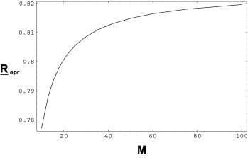
Figure 17: Quantum lower-bound $\underline{R}_{epr}$ versus the bandwidth $M$ of the EPR transmitter. Other parameters are $r_{0}=0.95$, $r_{1}=1,$ $N=100$, $m=2000$ and $\varepsilon=10^{-9}$. The curve represents a lower-bound for the rate (information bits per cell) which is achievable by an EPR transmitter $T_{M,N}$ combined with an optimal EC code.

In conclusion, we have considered alternative models of memories where the information is stored in EC blocks in such a way that the readout is almost flawless. In the regime of high reflectivities and few photons, we have checked that narrowband EPR transmitters are able to retrieve the logical data with a small EC overhead. By contrast, using classical transmitters in the same situation is completely unfeasible since the corresponding EC overhead is huge (more than $100$ cells to store a bit of information). This would imply reading times $100$ times longer and logical capacities $100$ times smaller. In other words, by reducing the number of photons, the classical readout becomes so noisy that no EC code is able to recover the stored information in an efficient way.

IX General Bounds for Error Correcting Codes

Here we recall two important bounds for EC codes. These bounds are used in Eq. (176).

Hamming Bound HammREF . 

For large $m$, an EC code $[m,k,d]$ has rate $R:=k/m$ and relative distance $\delta:=d/m$ such that

$$R\leq 1-H(\delta/2)+O(1/m)~{},$$ (179)

where $H$ is the binary Shannon entropy [defined in Eq. (177)].

Gilbert-Varshamov Bound GilbertREF ; VarshaREF . 

For large $m$ and $0\leq\delta\leq 1/2$, there exists an EC code with rate

$$R\geq 1-H(\delta)+O(1/m)~{},$$ (180)

where $H$ is the binary Shannon entropy [defined in Eq. (177)].

X Conclusive Discussions

X.1 Implications of the Few-Photon Regime

The advantages of quantum reading are related with the regime of few photons, roughly given by $N\simeq 1\div 10^{2}$ photons per cell. Note that this is very far from the energy which is used in today’s classical readers, roughly given by $N\simeq 10^{10}$ photons per cell Trates ; DVDbook . In order to understand the advantages connected with the few-photon regime, let us fix the mean signal power $P_{S}$ which is irradiated over the cell during the reading time. This quantity is approximately

$$P_{S}=(h\nu)\frac{N}{t}~{},$$ (181)

where $h$ is the Planck’s constant, $\nu$ is the carrier frequency of the light, $N$ is the mean number of photons in the signal, and $t$ is the reading time of the cell. According to Eq. (181), for fixed power $P_{S}$, we can decrease $N$ together with $t$. In other words, the regime of few photons can be identified with the regime of short reading times, i.e., high data-transfer rates. Thus our results indicate the existence of quantum transmitters which allow reliable fast readout of digital memories.

Another implication of the few-photon regime is the increase of the storage capacity. As long as the carrier frequency $\nu$ of the reading light is able to resolve each single cell, we can increase the storage capacity just as a consequence of the increased data-transfer rates. In other words, because of the shorter reading time of the cell, we can increase the number of cells per area unit (density) while keeping the total reading time of the disk as constant. This is possible until the linear size of each cell is much larger than the wavelength of the light. For higher densities, we have to increase the frequency of the light in order to avoid diffraction and still use our model. It is clear that using frequencies above the visible range will involve the development of appropriate quantum sources. Note that the increase in the memory density can also be explained as a consequence of Eq. (181). In fact, for fixed power $P_{S}$, we can decrease $N$ while increasing $\nu$. This means that the regime of few photons can also be identified with the regime of high frequencies, i.e., high densities. Thus there exist quantum transmitters which can read, reliably, dense digital memories.

The previous physical discussion (done for fixed signal power $P_{S}$) can be generalized to include the “price to pay” for generating the light source. Given a global initial power $P$, we can write $P_{S}=\kappa P$, where the conversion factor $\kappa$ depends on the source to be generated: typically $\kappa\simeq 1$ for classical light, while $\kappa\ll 1$ for non-classical light. Then, for fixed $P$, we have reading times $t=O(\phi)$ where $\phi:=N/\kappa$. Here the ratio $\phi$ can still be advantageous for quantum reading thanks to its superiority in the few-photon regime. For instance, today’s CDs are classically read using $N\simeq 10^{10}$ photons per cell, so that $\phi_{\text{{class}}}\simeq 10^{10}$ Trates ; DVDbook . Using spontaneous parametric down conversion in periodically poled KTP waveguides Fiorentino we can generate EPR correlations around $810$ nm with $\kappa\simeq 10^{-9}$. Exploiting this quantum source in the few-photon regime, e.g., $N\simeq 1$, we can get $\phi_{\text{{quant}}}\simeq 10^{9}$, thus realizing shorter reading times. Clearly, this is a very rough estimate. However, this improvement will become more and more evident as technology provides cheaper ways to create non-classical light (see, e.g., the recent achievements of TPE ).

X.2 Towards a Pilot Experiment

It is important to note that the discussions of Sec. X.1 represent general theoretical predictions, mainly based on the simple formula of Eq. (181). More detailed evaluations are needed for an experimental implementation of the scheme, where all the technicalities must be taken into account. From this point of view it is interesting to attempt an evaluation of the current technological facilities in order to realize a first pilot experiment able to show the potentialities of quantum reading. In the following we provide a semi-quantitative estimate of the data-transfer rates that we could achieve by exploiting the current facilities in quantum technology.

First of all, note that a possible way to realize quantum reading is in the time domain, where different modes correspond to different laser pulses. Thus, we can consider an EPR transmitter $T_{M,N}$ emitting $M$ couples of entangled pulses which irradiate a total of $N$ photons over the cell. Let us assume that each pulse has duration $\tau=w^{-1}$, where $w$ is the spectral bandwidth (around a carrier frequency $\nu\gg w$). Then the minimum reading time of the cell is $t=M\tau$. Its inverse $R=t^{-1}$ gives the maximum data-transfer rate (in terms of bits per second). This value of the rate is however a rough estimate. In the experimental practice, the pulses do not satisfy the minimum time-bandwidth product relationship ($\tau w=1$), and the data-transfer rate is better given by $R=R^{\prime}/M$, where $R^{\prime}$ is the experimental pulse repetition rate (pulses per second), and $M$ is the number of pulses per cell. Today it is possible to generate femtosecond pulses of strongly entangled photons with high repetition rates. For instance, in Refs. Kri ; Pan , commercial mode-locked Ti:sapphire lasers are used to generate 100-fs pulses at 780-810 nm with repetition rates of 76-81 MHz. Using non-linear crystals, each of these pulses is first frequency-doubled and then down-converted (via SPDC) in two entangled pulses. The overall process is clearly inefficient. However, if we use strong input powers the output entangled pulses are populated with about one photon per pulse Pan . This means that we can generate TMSV states with sufficient squeezing at the optical-infrared frequencies with high repetition rates (e.g., $R^{\prime}=80$ MHz). Using $M$ of these states, we can construct an EPR transmitter emitting $M$ pulses and signal-energy $N=zM$ where $z\simeq 1$ (since we can have roughly one photon per pulse impinging on the cell Pan ). Thus, for the quantum reading scheme, we can consider $R=zR^{\prime}/N$ where $z\simeq 1$ photons per pulse, $R^{\prime}$ is around 80 MHz (pulses per second), and $N$ is the mean total number of photons per cell. This estimate must be further corrected by considering other technical issues. First, we have to introduce a factor $y<1$ accounting for non-ideal quantum efficiencies of the output detectors. Thus, we have to consider the lower rate $R=yzR^{\prime}/N$. In order to evaluate $y$, the fundamental measurement is the time-domain homodyne detection. This is in fact the measurement at the basis of our sub-optimal receiver design of Sec. VII (when it is supposed to work in the time domain.) Time-resolved homodyne detections have been recently studied by several experimental groups Han ; Wen ; Wenb ; Had ; Zav ; Zavb ; Zavc . According to Refs. Had ; Zav ; Zavb ; Zavc , it is possible to realize time-resolved homodyne detections at the optical-infrared frequencies (786-800 nm) with high repetition rates (54-82 MHz) and high signal-to-noise ratios (12dB). In particular, at repetition rates around 80 MHz, we can still have acceptable quantum efficiencies, e.g., $y\simeq 0.6$ according to Ref. Zavc . Finally, there is also the effect of classical error correction. On average, the readout of a single cell corresponds to decoding $x<1$ logical bits, which leads to the further correction $R=xyzR^{\prime}/N$. As discussed in the previous Sec. VIII, we can decode $x\simeq 0.8$ information bits per cell by employing good error correcting codes (see Fig. 17 and previous Sec. VIII for details). Thus, for the quantum reading of high reflectivity memories, we can consider $R=xyzR^{\prime}/N$ where $x\simeq 0.8$, $y\simeq 0.6$, $z\simeq 1$ and $R^{\prime}\simeq 80~{}$MHz. The resulting data-transfer rate $R\simeq 38/N$ (Mbit/s) is inversely proportional to the number of photons $N$. By assuming $N$ in the range of 1-70 photons, we have $R$ ranging between 0.5 Mbit/s and 38 Mbit/s. This is already comparable with the data-transfer rates of current optical memories. For instance, in today’s CDs, we have $R=1.23$ Mbit/s at the basic speed of 1X, and $R=70$ Mbit/s at the speed of 56X (see, e.g., Wikipedia). Thus, quantum reading can already provide good data-transfer rates by exploiting present facilities in ultra-fast quantum technology.

It is clear that this technique has the potential to become much faster as quantum technology provides better quantum sources and faster quantum detectors. As a matter of fact new efficient ways for producing entanglement have been recently developed. A very promising method is the two-photon-emission from semiconductors TPE . According to Ref. TPE , the pair-generation rate in GaAs/AlGaAs quantum well structure is estimated to be 3 orders of magnitude higher than for traditional broadband parametric down-conversion sources. By exploiting new sources of this kind, quantum reading has the long-term potential to go far beyond any data-transfer rate which is achievable by classical devices.

X.3 Application to Photodegradable Media

Besides the potentialities previously described, there is another interesting application of quantum reading in the few-photon regime: the safe readout of photodegradable memories. These are memories where faint quantum light can retrieve the data safely, while classical light could only be destructive. Memories of this kind could be constructed on purpose. For instance, we could construct extremely photo-sensitive organic microfilms which melt under very few photons of visible light. An agency could use these cryptographic devices to store confidential information. Their security would rely on the technological complexity of the corresponding readers (e.g., extremely precise quantum readers held by the agency only.)

Other examples of photodegradable memories are dye-based optical disks. Since we can read information using few photons, we could construct and make use of optical disks which are composed of extremely photo-sensitive dyes or other similar organic materials. The problem of dye-degradation is very important and involves current optical disks too. In today’s recordable optical media (CD-R and DVD-R), the data is recorded in internal layers of organic dye (e.g., Azo, Cyanine, or Phthalocyanine) by means of a writing process called “dye-sublimation” DVDbook ; NOTA3 . The long-term use of these memories seems to be restricted to visible frequencies, since their organic layers undergo a rapid UV-degradation at higher frequencies DVDbook ; UV . In other words, despite organic disks of higher densities could be written, their first readout could be completely destructive as a result of the UV-degradation. In this scenario the use of faint quantum light could provide a safe and reliable readout, thus enabling these memories to be developed to higher densities. Clearly this is possible after the development of appropriate non-classical sources in the UV range. Thus, from this perspective, our work shows new possible directions in the technology of organic memories.

More generally, the results of quantum reading can be applied to the study of photodegradable absorbing materials. Whenever two absorbing media can be modeled by two attenuator channels with different losses, their discrimination is equivalent to the readout of an information bit from a memory cell (according to our basic model of memory). If these media are furthermore photodegradable, then the use of faint quantum light could represent the only method to solve their discrimination without destroying the sample.

References

- (1) M. A. Nielsen and I. L. Chuang, Quantum Computation and Quantum Information (Cambridge University Press, Cambridge, 2000).
- (2) S. L. Braunstein and A. K. Pati, Quantum Information Theory with Continuous Variables, (Kluwer Academic, Dordrecht, 2003).
- (3) S. L. Braunstein and P. van Loock, Rev. Mod. Phys. 77, 513 (2005).
- (4) A. Ferraro, S. Olivares, and M. Paris, Gaussian states in quantum information, ISBN 88-7088-483-X (Biliopolis, Napoli, 2005); J. Eisert and M. B. Plenio, Int. J. Quant. Inf. 1, 479 (2003).
- (5) For any -mode bosonic state , we can write the -representation , where is normalized to and is a multimode coherent state. Then, is called “classical” (“non-classical”) if is positive (non-positive) Prepres . For classical, is a probability distribution (implying separability).
- (6) E. C. G. Sudarshan, Phys. Rev. Lett. 10, 277 (1963); R. J. Glauber, Phys. Rev. 131, 2766 (1963).
- (7) A. Einstein, B. Podolsky, and N. Rosen, Phys. Rev. 47, 777 (1935).
- (8) For two bosonic modes, and , with quadratures , , and , one can define the two operators (relative position) and (total momentum). Then, the system has EPR correlations (in these operators) if , where is the variance, and is the standard quantum limit ( in this paper.) A bosonic system with EPR correlations is entangled, but the contrary is not necessarily true. In today’s quantum optics labs, the EPR correlations represent the standard type of continuous variable entanglement. These correlations are usually generated via spontaneous parametric down conversion.
- (9) H. P. Yuen, and R. Nair, Phys. Rev. A 80, 023816 (2009).
- (10) S.-H. Tan et al., Phys. Rev. Lett. 101, 253601 (2008); S. Lloyd, Science 321, 1463 (2008).
- (11) In our Letter, is always a mean quantity (averaged over the state). It represents the mean number of photons in the whole -mode signal system. Clearly, the ratio gives the mean number of photons per signal mode.
- (12) K. M. R. Audenaert et al., Phys. Rev. Lett. 98, 160501 (2007).
- (13) S. Pirandola and S. Lloyd, Phys. Rev. A 78, 012331 (2008).
- (14) is a sufficient condition for the superiority of quantum reading. corresponds to the singular case where only quantum light can retrieve information.
- (15) C. F. Bohren, and D. Huffman, Absorption and scattering of light by small particles (John Wiley, New York, 1983).
- (16) With the notation we mean a matrix with entries , where . Analogously, is a matrix with entries .
- (17) R. Simon, N. Mukunda, and B. Dutta, Phys. Rev. A 49, 1567 (1994).
- (18) S. Pirandola, A. Serafini, and S. Lloyd, Phys. Rev. A 79, 052327 (2009).
- (19) G. Milburn and D. Walls, Quantum Optics (Springer 1994).
- (20) A. S. Holevo, Prob. of Inf. Transm. 43, 1 (2007).
- (21) S. Pirandola, S. L. Braunstein, and S. Lloyd, Phys. Rev. Lett. 101, 200504 (2008).
- (22) A. Serafini, J. Eisert, and M. M. Wolf, Phys. Rev. A 71, 012320 (2005).
- (23) C. W. Helstrom, Quantum detection and estimation theory (Academic Press, New York, 1976).
- (24) Note that in our Letter we use the short-hand notation .
- (25) In other words, projects onto the subspace spanned by the eigenstates of with positive eigenvalues.
- (26) We use the notation .
- (27) C. A. Fuchs and J. V. de Graaf, IEEE Trans. Inf. Theory 45, 1216 (1999).
- (28) C. Fuchs, PhD thesis (Univ. of New Mexico, Albuquerque, 1995).
- (29) H. Scutaru, J. Phys. A 31, 3659 (1998).
- (30) Jensen’s inequality states that, for every random variable , with values in and expectation value , and for any concave function , we have (the inequality is reversed for convex functions). More in general, the inequality holds for random variables and concave functions which are defined in measurable subsets .
-
(31)
Numerical investigations can also be performed by using the
simpler quantity
which is based on the quantum Battacharyya bound. - (32) S. Guha and B. Erkmen, Phys. Rev. A 80, 052310 (2009).
- (33) F. J. MacWilliams, and N. J. A. Sloane, The Theory of Error-Correcting Codes (North-Holland, 1977).
- (34) E. N. Gilbert, A comparison of signalling alphabets, Bell Syst. Tech. J. 31, pp. 504–522 (1952).
- (35) R. R. Varshamov, Estimate of the number of signals in error correcting codes, Dokl. Acad. Nauk 117, pp. 739–741 (1957).
- (36) A single-layer CD with speed 1X (i.e., 500 rpm) has a data-transfer rate of 1.23 Mbit/s. This data is read by a laser diode at 780 nm and power mW, therefore irradiating about nJ per bit. A higher-speed CD needs a laser with proportionally more power, in such a way that at least nJ per bit is irradiated, corresponding to photons per bit. By neglecting the error correction overhead, this corresponds to photons per cell.
- (37) J. Taylor, M. R. Johnson, and C. G. Crawford, DVD demystified (McGraw-Hill, 2005). See also Wikipedia.
- (38) For the sake of simplicity, we consider here the pure-loss model. As before, the derivation can be extended to the thermal-loss model and the sub-optimal receiver.
- (39) Note that this formula provides the expression of Eq. (175) when we set odd and (properties of the repetition codes).
- (40) M. Fiorentino et al., Opt. Express 15, 7479 (2007).
- (41) A. Hayat et al., Nature Photonics 2, 256 (2008).
- (42) R. Krischek, W. Wieczorek, A. Ozawa, N. Kiesel, P. Michelberger, T. Udem, and H. Weinfurter, Nature Photonics 4, 170-173 (2010).
- (43) D. Pan, W. Donaldson, and R. Sobolewski, Proc. SPIE 6583, 65830K (2007).
- (44) H. Hansen et al., Opt. Lett. 26, 1714-1716 (2001).
- (45) J. Wenger et al., Opt. Lett. 29, 1267-1269 (2004).
- (46) J. Wenger et al., Eur. Phys. J. D 32, 391-396 (2005).
- (47) O. Haderka et al., Applied Optics 48, 2884-2889 (2009).
- (48) A. Zavatta et al., J. Opt. Soc. Am. B 19, 1189-1194 (2002).
- (49) A. Zavatta et al., Phys. Rev. A 70, 053821 (2004).
- (50) A. Zavatta et al., Laser Phys. Lett. 3, 3-16 (2006).
- (51) During the writing process, a high-power laser heats the dye polymer which therefore darkens, with the result of causing less reflection from the metallic layer underneath.
- (52) http://en.wikipedia.org/wiki/UV_degradation.