Entanglement and localization of wavefunctions

Abstract

We review recent works that relate entanglement of random vectors to their localization properties. In particular, the linear entropy is related by a simple expression to the inverse participation ratio, while next orders of the entropy of entanglement contain information about e.g. the multifractal exponents. Numerical simulations show that these results can account for the entanglement present in wavefunctions of physical systems.

I Introduction

Quantum mechanics has always seemed puzzling since its first construction in the first half of the XXth century. Many properties are different from the world of classical physics in which our intuition is built. The development of quantum information science in the last decades has exemplified this aspect. Indeed, it was realized that it is in principle possible to exploit the features of quantum mechanics to treat information in a different way from what a classical computer would do. In this context, the specific properties of quantum mechanics are put forward as new resources which enable to treat information in completely new ways.

One of the most peculiar properties of quantum mechanics is entanglement, that is the possibility to construct quantum states of several subsystems that cannot be factorized into a product of individual states of each subsystem. Such entangled states are the most common in quantum mechanics, and they display correlations which cannot be seen in a classical world, exemplified by e.g. the Einstein-Podolsky-Rosen “paradox”. Entanglement is also a resource for quantum information (see nielsen and references therein), and has been widely studied as such in the past few years.

Despite intensive work, entanglement remains a somewhat mysterious property of physical systems. The structure of entanglement of systems even with small numbers of particles is hard to characterize. Even properly measuring the entanglement present in a system is difficult for mixed states. This is all the more important since recent results have shown that (at least for pure states) if a process creates a sufficiently low level of entanglement, it can be simulated efficiently by a classical computer jozsa . This gives a limit on the speedup over classical computation a quantum computer can achieve, and also gives rise to interesting proposals for building classical algorithms simulating weakly entangled quantum systems cirac .

In this paper, we review recent results we obtained (details can be found in GMG1 ; GMG2 ), which concern the relationship of entanglement to localization properties of a quantum state. Our strategy is to consider $n$-qubit systems, and to study entanglement of quantum states relative to their localization properties in the $2^{n}$-dimensional Hilbert space in the computational basis. We obtain analytical results for random states, that is ensemble of quantum states sharing some properties. Such random states have been recently studied in the literature. They are interesting in themselves, since it has been shown for example in quantum information that they are useful in various quantum protocols random . This motivated a recent activity in the quantum information community to try and produce efficiently such random vectors or random operators through quantum algorithms emerson , and to characterize their entanglement properties ranvec . In addition to their intrinsic usefulness, random states are important since they can describe typical states of a ”complex” system. For example, it has been known for some time now that random vectors built from Random Matrix Theory (RMT) can describe faithfully the properties of quantum Hamiltonian systems whose classical limit is chaotic, and more generally of many complex quantum systems houches . Such random vectors are ergodic, and the entanglement they contain has been calculated some time ago Lub ; Pag . However, in many quantum systems, the wavefunctions are not ergodic but localized. This can correspond to electrons in a disordered potential, which are exponentially localized due to Anderson localization. It can also be seen in many-body interacting systems, where the presence of a moderate interaction can lead to states partially localized in energy. Some systems are in a well-defined sense neither ergodic neither localized: they correspond to e.g. states at the Anderson transition between localized and delocalized states, and can show multifractal properties mirlin .

In this paper, we calculate the amount of entanglement present in ensembles of random vectors displaying these various degrees of localization. Besides generalizing the result for RMT-type random vectors, this gives the entanglement present in a “typical state” of such localized or partially localized systems. This enables to estimate the complexity of simulating such systems on classical computers, but also sheds light on the entanglement itself, since in these cases it is related through simple formulas to quantities characterizing the degree of localization of the system.

Our results show that for random vectors which are localized on the computational basis, the linear entropy which approximates the amount of entanglement in the vector is simply related to the Inverse Participation Ratio (IPR), a popular measure of localization. The next term in the approximation is related to higher moments, and in particular to the multifractal exponents for multifractal systems. In order to assess the usefulness of these results to physical systems, we compare them to the entanglement numerically computed for several models. After a general discussion on entanglement of random vectors (section II), we consider the entanglement of one qubit with the others (section III), and give explicitly the first and second order of the expansion of the entropy of entanglement around its maximum. Section IV generalizes these results to other bipartitions, and section V compares the formula obtained with the numerical results for two physical systems. Section VI considers the physically important case of vectors localized not on a random subset of the basis vectors, but on a subset composed of adjacent basis vectors (that is the states are localized on computational basis states which are adjacent when the basis vectors are ordered according to the number which labels them), showing that the results become profoundly different. Section VII presents the conclusions.

II Entanglement of random vectors

Random vectors are ensembles of vectors whose components are distributed according to some probability distribution. If for example the system considered is composed of $n$ qubits, the Hilbert space is of dimension $N=2^{n}$. If the two states of a qubit are denoted $|0\rangle$ and $|1\rangle$, each state in the computational basis corresponds to a sequence of $0$ and $1$ and thus can be labelled naturally by a number between $0$ and $2^{n}-1$, and quantum states can be expanded as $|\psi\rangle=\sum_{i}\psi_{i}|i\rangle$. Random vectors distributed according to the uniform measure on the $N$-dimensional sphere describe typical quantum states of the $n$ qubits. Such states are ergodically distributed in the computational basis, and their entanglement has already been studied in Lub ; Pag . In this paper, we are interested in random vectors which are not ergodically distributed. Ensembles of such states will be characterized by localization properties. The simplest example of such localized random vectors can be constructed by taking $M$ components ($M<N$) with equal amplitudes and uniformly distributed random phases, and setting all the others to zero. The random vectors will all be exactly localized on $M$ basis states. A more physically relevant example consists in still choosing $M<N$ nonzero components, and giving them the distribution of column vectors of $M\times M$ random unitary matrices drawn from the Circular Unitary Ensemble of random matrices (CUE vectors). In general our result will be averaged both over the distribution of the nonzero components and the position of these nonzero components in the computational basis. This corresponds to classes of random vectors sharing the same localization length. Our results will in fact generalize to any such distribution of random vectors whose localization properties are fixed. In addition, we shall see that if we impose that the distribution of the indices $i$ of nonzero components $\psi_{i}$ is such that they are always adjacent in the computational basis (i.e. the indices $i$ are consecutive integers), the results change drastically.

The localization properties of the random vectors can be probed using the moments of the distribution

$$p_{q}=\sum_{i=1}^{N}|\psi_{i}|^{2q}.$$ (1)

The second moment is $p_{2}=1/\xi$, where $\xi$ is the Inverse Participation Ratio (IPR) which is often used in the mesoscopic physics literature to measure the localization length. Indeed, for a state uniformly spread on exactly $M$ basis vectors, one has $\xi=M$. The scaling of $p_{2}$ and higher moments with the size also probes the multifractal properties of the wavefunction.

The random states we consider are built on the $N$-dimensional Hilbert space of a $n$-qubit system with $N=2^{n}$. We are interested in bipartite entanglement between subsystems defined by different partitions of the $n$ qubits into two sets. In general, bipartite entanglement of a pure state belonging to a Hilbert space ${\mathcal{H}}_{A}\otimes{\mathcal{H}}_{B}$ is measured through the entropy of entanglement, which has been shown to be a unique entanglement measure PopRoh . We consider pure states belonging to ${\mathcal{H}}_{A}\otimes{\mathcal{H}}_{B}$ where ${\mathcal{H}}_{A}$ is a set of $\nu$ qubits and ${\mathcal{H}}_{B}$ a set of $n-\nu$ qubits. If $\rho_{A}=\textrm{tr}_{B}|\psi\rangle\langle\psi|$ is the density matrix obtained by tracing out subsystem $B$, then the entropy of entanglement of the state $\psi$ with respect to the bipartition $(A,B)$ is the von Neumann entropy of $\rho_{A}$, that is $S=-\textrm{tr}(\rho_{A}\log_{2}\rho_{A})$.

III Entanglement of one qubit with all the others

To obtain an approximation for the entropy, one can expand $S$ around its maximal value. In the case of the partition of the $n$ qubits into $1$ and $n-1$ qubits, the entropy can be written as a function of $\tau$, with

$$\tau=4\det\rho_{A}$$ (2)

(in the case of 2 qubits this quantity is called the tangle and corresponds to the square of the generalized concurrence RunCav ). One has

$$S(\tau)=h\left(\frac{1+\sqrt{1-\tau}}{2}\right),$$ (3)

where $h(x)=-x\log_{2}x-(1-x)\log_{2}(1-x)$. The series expansion of $S(\tau)$ up to order $m$ in $(1-\tau)$ reads

$$S_{m}(\tau)=1-\frac{1}{\ln 2}\sum_{n=1}^{m}\frac{(1-\tau)^{n}}{2n(2n-1)}.$$ (4)

The first order corresponds to $\tau$ itself up to constants and its average over the choice of the $(1,n-1)$ partition is known as the linear entropy or Meyer-Wallach entanglement $Q$ MW . Our results show that for our class of random vectors, the average linear entropy is given by

$$\langle\tau\rangle=\frac{N-2}{N-1}(1-\langle p_{2}\rangle)=\frac{N-2}{N-1}(1-\langle 1/\xi\rangle).$$ (5)

This formula was obtained first by considering a random vector which is nonzero only on $M$ basis vectors among $N$, and summing explicitly the combinatorial terms. It can also be obtained in a more general setting by taking $M=N$ and summing up all the localization properties of the vector in the IPR $\xi$ alone. For any $(1,n-1)$ partition of the $n$ qubits, the components of the vector can be divided in two sets according to the value of the first qubit. Assuming no correlation among these sets enables to get Eq. (5) (details on the calculations can be found in GMG1 ).

It is interesting to compare this formula with a similar one obtained in viola using different assumptions, in particular without average over random phases. The formula obtained relates entanglement to the mean inverse participation ratio calculated in three different bases, a quantity that is more general but often delicate to evaluate. In our case, the additional assumption of random phases enables to obtain a formula which involves only the IPR in one basis, a quantity that can be easily evaluated in many cases. For example, it enables to compute readily the entanglement for localized CUE vectors. However there are instances of systems (e.g. spin systems) where these different formulas give the same results.

In particular, our formula (5) allows to compute $\langle\tau\rangle$ e. g. for a CUE vector localized on $M$ basis vectors; in this case $\xi=(M+1)/2$, and we get

$$\langle\tau\rangle=\frac{M-1}{M+1}\frac{N-2}{N-1}.$$ (6)

In Lub , $\langle\tau\rangle$ was calculated for non-localized CUE vectors of length $N$, giving $\langle\tau\rangle=(N-2)/(N+1)$. Consistently, our formula yields the same result if we take $M=N$. For a vector with constant amplitudes and random phases on $M$ basis vectors, $\xi=M$ and

$$\langle\tau\rangle=\frac{M-1}{M}\frac{N-2}{N-1}.$$ (7)

Thus the first order of the expansion, which gives the main features of the entanglement, has very simple expressions in term of system parameters.

The next order in the expansion (4) can be obtained by similar methods that we do not detail here (see GMG2 for details); summing up all terms involved in $\tau^{2}$ we get

$$\langle\tau^{2}\rangle = N(N-2)(N^{2}-6N+16)c_{1111}$$

$$+4N(N-2)(N-4)c_{211}+4N(N-2)c_{22}$$

with

$$c_{22} = \frac{\langle p_{2}^{2}\rangle-\langle p_{4}\rangle}{N(N-1)},\ c_{211}=\frac{\langle p_{2}\rangle-\langle p_{2}^{2}\rangle-2\langle p_{3}\rangle+2\langle p_{4}\rangle}{N(N-1)(N-2)},$$

$$c_{1111} = \frac{1-6\langle p_{2}\rangle+8\langle p_{3}\rangle+3\langle p_{2}^{2}\rangle-6\langle p_{4}\rangle}{N(N-1)(N-2)(N-3)}.$$ (9)

This gives the next order of the entropy of entanglement in terms of the moments up to order 4 of the vector. What this means is that at this order, the average entanglement of random vectors with fixed moments will be related to them through (III). Although more complicated than (5), the formula indicates that e.g. for states having multifractal properties, since moments scale with system size according to quantities called multifractal exponents, the behavior of the entanglement at this order will be also controlled by these multifractal exponents.

The $n$th order of the expansion (4) can similarly be obtained and has been derived in GMG2 . It is interesting to note that in the case of a CUE random vector of size $N$, resummation of the whole series for $S(\tau)$ yields, after some algebra,

$$\langle S(\tau)\rangle=\frac{1}{\ln 2}\sum_{k=N/2+1}^{N-1}\frac{1}{k},$$ (10)

which has been obtained earlier by a different method Pag .

A general conclusion obtained from these formulas is that the entanglement associated to such bipartition $(1,n-1)$ goes to the maximal value for large $N$ and large $\xi$, even if $\xi$ grows more slowly than $N$. For fixed $\xi$, it tends for large $N$ to a constant nonzero value which depends on $\xi$. We will see in Section VI that this result can change drastically if we impose a localization on fixed locations in Hilbert space.

IV Entanglement of random vectors: other partitions

Up to now we have considered the entanglement of one qubit with all the others, i.e. the $(1,n-1)$ partition of $n$ qubits. What about bipartite entanglement relative to other bipartitions $(\nu,n-\nu)$, where $\nu$ is any number between $1$ and $n-1$? In this case, it is convenient to define the linear entropy as $S_{L}=\frac{d}{d-1}(1-\textrm{tr}\rho_{A}^{2})$, where $d=\dim{\mathcal{H}}_{A}\leq\dim{\mathcal{H}}_{B}$. The scaling factor is such that $S_{L}$ varies in $[0,1]$.

A similar calculation as above enables then to obtain the first order of the mean von Neumann entropy. It is given by

$$\langle S\rangle\approx\nu-\frac{2^{\nu}-1}{2\ln 2}\left(1-\frac{N-2^{\nu}}{N-1}\Big{\langle}\frac{1}{\xi}\Big{\rangle}\right),$$ (11)

with $p_{2}=1/\xi$, which generalizes Eq. (5).

Higher-order terms can be obtained as well, although the calculations become tedious. To this end, the entropy $S=-\textrm{tr}(\rho_{A}\log_{2}\rho_{A})$ is expanded around the maximally mixed state $\rho_{0}=\mathbf{1}/2^{\nu}$, as

$$S=\nu+\frac{1}{\ln 2}\sum_{n=1}^{\infty}\frac{(-2^{\nu})^{n}}{n(n+1)}\textrm{tr}((\rho_{A}-\rho_{0})^{n+1}),$$ (12)

and the traces can be evaluated as sums over correlators of higher moments GMG2 .

We remark that again the linear entropy (11) tends to the maximal possible value when $N$ and $\xi$ become large, as for the $(1,n-1)$ partition.

V Entanglement of random vectors: application to physical systems

In order to test these results on physical systems, we compared them to numerical results obtained from different models.

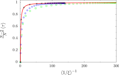
Figure 1: Scaled mean linear entropy $\langle\tau\rangle(N-2)/N$ of (13) vs mean IPR for $\delta=\Delta_{0}$, $n=10$ (blue circles) and $n=11$ (green squares). Red line is the theory, stars the data for $n=10$ with random shuffling of components (from GMG1 ).

The first one corresponds to a diagonal Hamiltonian matrix to which a two-body interaction is added.

$$H=\sum_{i}\Gamma_{i}\sigma_{i}^{z}+\sum_{i<j}J_{ij}\sigma_{i}^{x}\sigma_{j}^{x}$$ (13)

This system can describe a quantum computer in presence of static disorder qchaos . Here the $\sigma_{i}$ are the Pauli matrices for the qubit $i$, the energy spacing between the two states of qubit $i$ is given by $\Gamma_{i}$, which are randomly and uniformly distributed in the interval $[\Delta_{0}-\delta/2,\Delta_{0}+\delta/2]$, and $J_{ij}$ uniformly distributed in the interval $[-J,J]$ represent a random static interaction. Entanglement of eigenvectors of this Hamiltonian was already considered in a different context in italians . It is known qchaos that in this model a transition to quantum chaos takes place for sufficiently large coupling strength $J$. In this regime, eigenvectors of (13) are spread over all noninteracting eigenstates (those of (13) for $J=0$, which coincide to the computational basis), but in a certain window of energy, and are distributed according to the Breit-Wigner (Lorentzian) distribution. Thus these wavefunctions are distributed among a certain subset of the computational basis, although they are not strictly zero outside it, and the distribution is not uniform, but rather Lorentzian. Nevertheless, our data show (see Figs. 1,2) that the behavior of the bipartite entanglement of eigenvectors of this model is well described by the results (5) and (11) derived for random vectors. The agreement becomes very accurate if the eigenvector components are randomly shuffled to lower correlations.

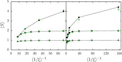
Figure 2: Mean entropy of entanglement $S$ for different bipartitions $(\nu,n-\nu)$ as a function of the mean IPR. Left: eigenvectors of (14) with $\gamma=1/3$; the average is taken over $10^{6}$ eigenvectors. Right: eigenvectors of (13) with $\delta=\Delta_{0}$ and $J/\delta=1.5$; average over $\approx 3\times 10^{5}$ vectors. Triangles correspond to $\nu=1$, squares to $\nu=2$ and circles to $\nu=n/2$, with $n=4-10$. Black symbols are the theoretical predictions for the mean value of $S$ (obtained from Eq. (11) and green (gray) symbols are the computed mean values of the von Neumann entropy (from GMG2 ).

We also considered another model, based on $N\times N$ matrices of the form

$$U_{kl}=\frac{e^{i\phi_{k}}}{N}\frac{1-e^{2i\pi N\gamma}}{1-e^{2i\pi(k-l+N\gamma)/N}},$$ (14)

where $\phi_{k}$ are random variables independent and uniformly distributed in $[0,2\pi[$ and $\gamma$ is a fixed parameter. This model introduced in bogomolny is the randomized version of a simple quantum map introduced in giraud . The eigenvectors of (14) have multifractal properties MGG for rational $\gamma$. The results of Figs. 2,3 show that again the results for random vectors describes very well the entanglement for this system for randomly shuffled components, and that even the first order is already a good approximation.

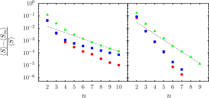
Figure 3: Relative difference of the entropy of entanglement (3) and its successive approximations $S_{m}$ ($m=1,2$) with respect to the number of qubits for eigenvectors of (14) for (left) $\gamma=1/3$ and (right) $\gamma=1/7$. The average is taken over $10^{7}$ eigenvectors, yielding an accuracy $\lesssim 10^{-6}$ on the computed mean values. Green triangles correspond to the first order expansion $S_{1}$, blue squares and red circles to the second order expansion $S_{2}$. The difference between the latter two is that for blue squares $\langle p_{2}^{2}\rangle$ appearing in Eq. (III) has been replaced by $\langle p_{2}\rangle^{2}$ yielding a less accurate approximation. Dashed line is a linear fit yielding $1-\langle S_{1}\rangle/\langle S\rangle$ $\sim N^{-0.84}$ for $\gamma=1/3$ and $N^{-1.58}$ for $\gamma=1/7$ (from GMG2 ).

VI Entanglement of adjacent random vectors

In the preceding sections we discussed formulas for entanglement of ensembles of random vectors where the components over each basis vector are independent. If we relax this assumption, the result may change. An important particular case corresponds e.g. to random vectors localized on $M$ computational basis states which are adjacent when the basis vectors are ordered according to the number which labels them (again, if the two states of a qubit are denoted $|0\rangle$ and $|1\rangle$, each state in the computational basis corresponds to a sequence of $0$ and $1$ and thus can be labelled naturally by a number between $0$ and $2^{n}-1$). In this case, we had to use combinatorial methods; summing all contributions together we get for the linear entropy of $(1,n-1)$ partitions

$$\langle\tau\rangle = \left[\left(\frac{M-2}{M-1}r_{0}+\frac{2(2^{r_{0}}-1)}{M(M-1)}+\frac{4}{3}\frac{(M+1)(2^{n}-2^{r_{0}})}{2^{n+r_{0}}}\right.\right.$$ (15)

$$-\left.\left.\frac{1}{M(M-1)}\sum_{r=0}^{r_{0}-1}\chi_{r}(m_{r})\right)\left(1-\langle\frac{1}{\xi}\rangle\right)\right]\frac{1}{n},$$

where $r_{0}$ is such that $2^{r_{0}-1}<M\leq 2^{r_{0}}$ and $\chi_{r}(x)=\chi_{r}(2^{r+1}-x)=x^{2}-\frac{2}{3}x(x^{2}-1)/2^{r}$ for $0\leq x\leq 2^{r}$. Equation (15) is an exact formula for $M\leq N/2$. For fixed $M$ and $n\rightarrow\infty$, $n\langle Q\rangle$ converges to a constant $C$ which is a function of $M$ and $\xi$. For $M=2^{r_{0}}$, $r_{0}<n$, Eq. (15) simplifies to

$$\langle\tau\rangle = \left[\left(\frac{(r_{0}+\frac{4}{3})M^{2}-2(r_{0}-1)M-\frac{10}{3}}{M(M-1)}\right.\right.$$ (16)

$$-\left.\left.\frac{4(M+1)}{3N}\right)\left(1-\langle\frac{1}{\xi}\rangle\right)\right]\frac{1}{n}.$$

Numerically, this expression with $r_{0}=\log_{2}M$ gives a very good approximation to Eq. (15) for all $M$.

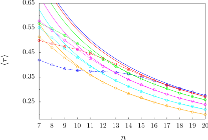
Figure 4: Mean linear entropy $\langle\tau\rangle$ of partitions $(1,n-1)$ vs number of qubits for the one-dimensional Anderson model with disorder from top to bottom $w=0.2$ (blue), $0.5$ (red), $1.0$ (green), $1.5$ (magenta), $2.0$ (cyan), and $2.5$ (orange). Average is over 10000 eigenstates. Solid lines are the $C/n$ fits of the tails (from GMG1 ).

Equation (15) is exact for e.g. uniform and CUE vectors, and can be applied even if the vector is not strictly zero outside a $M$-dimensional subspace. Indeed, for $N$-dimensional CUE vectors with exponential envelope $\exp(-x/l)$, $\langle Q\rangle$ is in excellent agreement with Eq. (15) with $\xi=l$ and $M=2\xi$.

In order to compare these findings to those of a physical system with such a property of localization on adjacent basis vectors, Fig. 4 shows the theory Eq. (15) together with the entropy for the one-dimensional Anderson model. This model corresponds to a one-dimensional chain of vertices with nearest-neighbor coupling and randomly distributed on-site disorder, described by the Hamiltonian $H_{0}+V$. Here $H_{0}$ is a diagonal operator whose elements $\epsilon_{i}$ are Gaussian random variables with variance $w^{2}$, and $V$ is a tridiagonal matrix with non-zero elements only on the first diagonals, equal to the coupling strength, set to $1$. It is known that eigenstates of this system, which modelizes electrons in a disordered potential, have envelopes of the form $\exp(-|x-x_{0}|/l)$, where $l$ is the localization length. It was shown in pomeransky that this model can be simulated efficiently on a quantum computer, and the wavefunction of the computer during the algorithm will be localized on adjacent basis vectors, which correspond to the position of vertices. Figure 4 shows that the asymptotic behavior of the linear entropy of the eigenstates (with all correlations left between components, i.e. no random shuffling) is well captured by Eq. (15).

Thus random vectors localized on adjacent basis vectors correspond to a drastically different behavior compared to the vectors of section III : indeed, for fixed $\xi$ the entanglement (at least the linear entropy) always tends to zero for large $N$, even if it does it rather slowly (as $\sim 1/\ln N$).

VII Conclusion

The results above indicate that the entanglement properties of random vectors can be directly related to the fact that they are localized, multifractal or extended. The numerical simulations for different physical systems show that these results obtained for random vectors describe qualitatively the entanglement present in several physical systems, and reproduce it accurately if correlations between components of the vector are averaged out.

Thus the results are interesting to predict the amount of entanglement present in random vectors, and also can be applied to physical systems for which such random vectors describe typical states. This gives insight on the difficulty to simulate classically such systems, since systems with low amounts of entanglement can be simulated classically efficiently. This also can be applied to estimate the changes in entanglement at a quantum phase transition spins , in particular for the Anderson transition between localized and extended states (see GMG2 for more details). Additionally, this gives also insight on the nature of entanglement itself by relating it to simple physical properties of the system.

- (1) M. A. Nielsen and I. L. Chuang, Quantum computation and quantum information, Cambridge Univ. Press, 2000.
- (2) R. Jozsa and N. Linden, Proc. R. Soc. London Ser. A 459, 2011 (2003); G. Vidal, Phys. Rev. Lett. 91, 147902 (2003).
- (3) G. Vidal, Phys. Rev. Lett. 91, 147902 (2003); F. Verstraete, D. Porras, and J. I. Cirac, Phys. Rev. Lett. 93, 227205 (2004).
- (4) O. Giraud, J. Martin, and B. Georgeot, Phys. Rev. A 76, 042333 (2007).
- (5) O. Giraud, J. Martin, and B. Georgeot, Phys. Rev. A 79, 032308 (2009).
- (6) A. Harrow, P. Hayden and D. Leung, Phys. Rev. Lett. 92, 187901 (2004); P. Hayden, D. Leung, P. Shor and A. Winter, Commun. Math. Phys. 250, 371 (2004); C. H. Bennett, P. Hayden, D. Leung, P. Shor and A. Winter, IEEE Trans. Inf. Theory 51, 56 (2005). P. Cappellaro, J. Emerson, N. Boulant, C. Ramanathan and D. G. Cory, Phys. Rev. Lett. 94, 020502 (2005).
- (7) J. Emerson, Y. S. Weinstein, M. Saraceno, S. Lloyd and D. S. Cory, Science 302, 2098 (2003); Y. S. Weinstein and C. S. Hellberg, Phys. Rev. Lett. 95, 030501 (2005).
- (8) A.J. Scott, Phys. Rev. A 69, 052330 (2004); H.-J. Sommers and K. Zyczkowski, J. Phys. A 37, 8457 (2004); O. Giraud, J. Phys. A 40, 2793 (2007); O. Giraud, J. Phys. A 40, F1053 (2007); M. Znidaric, J. Phys. A 40, F105 (2007); M. Znidaric, T. Prosen, G. Benenti and G. Casati, J. Phys. A 40, 13787 (2007); P. Facchi, U. Marzolino, G. Parisi, S. Pascazio and A. Scardicchio, Phys. Rev. Lett. 101, 050502 (2008).
- (9) Chaos and quantum physics, Proceedings of the 52th Les Houches Summer School, Eds. M.-J. Giannoni, A. Voros and J. Zinn-Justin (North-Holland, Amsterdam,1991).
- (10) E. Lubkin, J. Math. Phys. (N.Y.) 19, 1028 (1978).
- (11) D. N. Page, Phys. Rev. Lett. 71, 1291 (1993).
- (12) A. D. Mirlin, Phys. Rep. 326, 259 (2000); F. Evers and A. D. Mirlin, arXiv:0707.4378.
- (13) S. Popescu and D. Rohrlich, Phys. Rev. A 56, R3319 (1997).
- (14) P. Rungta and C. M. Caves, Phys. Rev. A 67, 012307 (2003).
- (15) A. D. Meyer and N. R. Wallach, J. Math. Phys. 43, 4273 (2002). G. K. Brennen, Quant. Inf. Comp. 3 619 (2003).
- (16) L. Viola and W. G. Brown, J. Math. Phys. 43, 8109 (2007); W. G. Brown, L. F. Santos, D. J. Starling and L. Viola, Phys. Rev. E 77, 021106 (2008).
- (17) B. Georgeot and D. L. Shepelyansky, Phys. Rev. E 62, 3504 (2000); ibid. 62, 6366 (2000).
- (18) C. Mejia-Monasterio, G. Benenti, G. G. Carlo and G. Casati, Phys. Rev. A 71, 062324 (2005).
- (19) E. Bogomolny and C. Schmit, Phys. Rev. Lett. 93, 254102 (2004).
- (20) O. Giraud, J. Marklof and S. O’Keefe, J. Phys. A 37, L303 (2004).
- (21) J. Martin, O. Giraud, and B. Georgeot, Phys. Rev. E 77, R035201 (2008).
- (22) A. A. Pomeransky and D. L. Shepelyansky, Phys. Rev. A 69, 014302 (2004); O. Giraud, B. Georgeot and D. L. Shepelyansky, Phys. Rev. E 72, 036203 (2005).
- (23) L. Amico, R. Fazio, A. Osterloh and V. Vedral, Rev. Mod. Phys. 80, 517 (2008).