Conductance of tubular nanowires with disorder

Abstract

We calculate the conductance of tubular-shaped nanowires having many potential scatterers at random positions. Our approach is based on the scattering matrix formalism and our results analyzed within the scaling theory of disordered conductors. When increasing the energy the conductance for a big enough number of impurities in the tube manifests a systematic evolution from the localized to the metallic regimes. Nevertheless, a conspicuous drop in conductance is predicted whenever a new transverse channel is open. Comparison with the semiclassical calculation leading to purely ohmic behavior is made.

1 Introduction

Electronic transport in nanostructures is often affected by the presence of impurities. Understanding impurity induced disorder has been a major concern in the field of quantum transport for many years. A vast literature on this problem has accumulated since Anderson’s discovery of the phenomenon of weak localization Anderson and the proposal of the scaling theory scaling . A lengthy introduction to the field is out of the scope of this work but the reader is addressed to Refs. rev1 ; rev2 ; rev3 ; rev4 for reviews on the topic.

In this paper we address a specific nanostructure geometry, namely a two-dimensional (2D) electron gas on the surface of a tube. Our motivation to study this particular nanostructure shape is mainly due to the similarity with rolled-up semiconductor quantum wells recently fabricated expertube ; et2 ; et22 ; et3 ; et4 and studied theotube ; tt2 ; tt3 . Here, it is also worth mentioning the apparent resemblance with electrons in carbon nanotubes, although these latter systems are generally of smaller dimensions. We also stress that this geometry is particularly adapted to the theoretical modeling of random impurities. Indeed, by means of longitudinal translations and rotations, i.e., the tube symmetries, one can always relate the position of two impurities on the tube surface.

We have implemented the numerical modeling of the disordered nanotubes using the scattering matrix formalism. In this approach, the solution of the Schrödinger equation is obtained by treating each scatterer as a black box characterized by its transmission and reflection amplitudes. The solution to the many impurity problem is then found by adequately composing the single impurity scattering matrices. Our approach is similar to that of Cahay, McLennan and Datta for planar wires cahay . A practical difference, however, is that we do not present the problem as a matrix recursion but, instead, as a global sparse linear system.

When increasing the number of propagating transverse modes the system behavior evolves from purely one dimensional (1D) in the one-mode limit towards 2D in the infinite-mode limit. In this paper we focus on the few-mode regime, or quasi-1D limit, monitoring the evolution of the conductance for energies allowing up to five propagating modes. In all cases the disordered wire is characterized by the asymptotic exponential localization of the wave function. However, it will be shown below that depending on the energy remarkable variations of the localization properties are predicted.

The scaling theory of disordered wires implies that, given a wire length $L$, wire conductance is a random variable $\tilde{G}$, characterized by a certain probability distribution $P_{L,\gamma}(\tilde{G})$. Randomness appears due to the infinite ways in which the number of impurities ${\cal N}$ can be arranged (each particular arrangement is usually referred as a disorder realization). Besides $L$, the probability distribution is also characterized by parameter $\gamma$, usually known as Lyapunov exponent rev2 . The relation between the Lyapunov exponent and the mean conductance strongly depends on the wire length. In other words, the form of $P_{L,\gamma}(\tilde{G})$ changes strongly with $L$. The precise definition of $\gamma$ involves averaging a function of the random conductance over all disorder realizations in the limit of a very long wire; namely

$$\gamma=\lim_{L\to\infty}{\langle\tilde{\gamma}\rangle}\;,$$ (1)

where we have defined

$$\tilde{\gamma}=\frac{1}{L}\log\left(1+\frac{G_{0}}{\tilde{G}}-\frac{1}{M}\right)\>.$$ (2)

In Eq. (2), $G_{0}\equiv 2e^{2}/h$ represents the conductance quantum and $M$ is the number of propagating modes in the wire. For a given $L$ and disorder realization the system is characterized by a single value of $\tilde{G}$ and its associated $\tilde{\gamma}$. Changing the disorder realization these variables acquire the statistical meaning implied above. Clearly, $\tilde{\gamma}$ is then a random variable whose mean, in the long wire limit, gives the Lyapunov exponent.

The inverse of the Lyapunov exponent gives the localization length $\ell=\gamma^{-1}$. This length is physically relevant since it specifies how $\tilde{G}$ and $\tilde{\gamma}$ are distributed for a given $L$. Two limiting regimes are known.

• $L\gg\ell$ (localized regime): $\tilde{\gamma}$ is normally (Gaussian) distributed with mean value $\gamma$ and width $\sigma^{2}_{\rm loc}=2\gamma/L$. In this limit we then have

  $$P_{L,\gamma}(\tilde{G})=\frac{1}{\sqrt{2\pi}\sigma_{\rm loc}}e^{-(\tilde{\gamma}-\gamma)^{2}/2\sigma^{2}_{\rm loc}}\frac{d\tilde{\gamma}}{d\tilde{G}}\;,$$ (3)

  where $\tilde{\gamma}$ as well as $d\tilde{\gamma}/d\tilde{G}$ can be obtained from $\tilde{G}$ using Eq. (2).

• $L\ll\ell$ (metallic regime): $\tilde{G}$ is normally distributed

  $$P_{L,\gamma}(\tilde{G})=\frac{1}{\sqrt{2\pi}\sigma_{\rm met}}e^{-(\tilde{G}-G)^{2}/2\sigma^{2}_{\rm met}}\;,$$ (4)

  with mean value given by

  $$G=\frac{G_{0}}{e^{\gamma_{L}L}-1+\frac{1}{M}}\;,$$ (5)

  and a constant variance. Indeed, universality in the value of $\sigma_{\rm met}$ is the reason why this limit is also dubbed the universal conductance fluctuation regime. In our case in which time reversal and spin rotation symmetries are fulfilled this value is $\sigma_{\rm met}=\sqrt{\frac{2}{15}}G_{0}$ rev1 . Notice that in Eq. (4) we have considered the possibility that the mean value $\gamma_{L}\equiv\langle\tilde{\gamma}\rangle$ may not be fully converged yet to the Lyapunov exponent for a given $L\ll\ell$.

Purely Ohmic behavior is characterized by a strict linearity of the resistance with the wire length. Such a behavior is obtained in a semiclassical description, where any possibility of quantum interference is neglected, and the scatterers are composed incoherently. Total transmission in this case does not depend on the impurity positions notesc , but only on its number ${\cal N}$ which is fixed for a certain length $L$. The semiclassical conductance $G_{\rm sc}(L)$ is then fully deterministic and can be written in terms of a single parameter $\alpha$ as

$$G_{\rm sc}(L)=\frac{G_{0}}{\alpha L+\frac{1}{M}}\;.$$ (6)

Deep in the metallic regime the mean quantum conductance also has an Ohmic behavior, as seen immediately from Eq. (5) assuming $\gamma_{L}=\gamma$ and expanding $e^{\gamma L}\approx 1+\gamma L$. Notice, however, that this Ohmic dependence may be different from the semiclassical one since we may have $\alpha\neq\gamma$, as will be shown below for particular cases. Including the next-order contribution from the exponential and assuming many propagating modes such that $\frac{1}{M}\ll\gamma L\approx\alpha L\ll 1$ we find

$$\langle\tilde{G}\rangle-G_{\rm sc}(L)=G_{0}\frac{(\alpha-\gamma)L-\frac{1}{2}(\gamma L)^{2}}{(\alpha L)(\gamma L)}\;.$$ (7)

If $\alpha=\gamma$, Eq. (7) predicts $\langle\tilde{G}\rangle=G_{\rm sc}(L)-G_{0}/2$, but this need not be true in general.

In this paper we calculate the localization length of disordered tubes and its evolution with energy covering from one to five propagating modes. The above prediction of scaling theory in the localized and metallic regimes is shown to be fulfilled and the deviation from it in the intermediate regime is explicitly shown. Given a number of propagating modes we find a steady increase of localization length with energy. Quite remarkably, however, a large drop is obtained each time a new mode becomes propagating. As pointed by Thouless thouless the localization length is related to the density of states and, therefore, we may expect some type of discontinuity in our quasi 1D system. This variation in localization length is the cause of similar drops in the mean conductance of a disordered tube of length $L$. In this case, increasing the energy the tube evolves from a more localized towards a more metallic regime.

The paper is organized as follows. In Sec. 2 we present the model and our approach to the many impurity scattering problem (in appendix we also discuss the solution of the single impurity problem). Section 3 contains the results and its discussion while Sec. 4 draws the conclusions of the work.

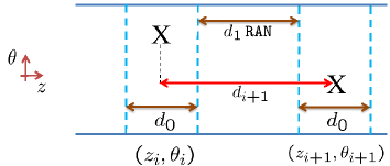
Figure 1: Parameters of the impurity distribution.

2 Model

We assume the electrons move on the surface of a cylinder of radius $\rho$. Disorder is represented by repulsive potential barriers mimicking the effect of impurities on the tube surface. The potential is assumed of a short range (Gaussian) type

$$V^{(i)}({\bf r})=V_{0}e^{-|{\bf r}-{\bf r}_{i}|^{2}/\sigma^{2}}\;,$$ (8)

where ${\bf r}_{i}$ is a specific impurity position. ${\cal N}$ such impurities, a rather large number, are present with positions $\left\{{\bf r}_{i},i=1,\dots,{\cal N}\right\}$. All impurities are assumed to be identical, although we would not expect qualitative differences in the results presented below if some variation in $V_{0}$ and $\sigma$ was considered.

2.1 Impurity distribution

Impurities are assumed to be well separated compared with the potential range $\sigma$. A sequential random distribution is then represented by the two parameters $d_{0}$ and $d_{1}$ (see a sketch in Fig. 1). The first impurity is arbitrarily positioned at $(z_{1},\theta_{1})=(0,0)$ and successive ones at

$$\left\{\begin{array}[]{rcl}z_{i}&=&z_{i-1}+d_{0}+d_{1}\,\verb+RAN+\\ \theta_{i}&=&2\pi\,\verb+RAN+\end{array}\right.\quad(i=2,\dots,{\cal N})\;,$$ (9)

where RAN is a standard random number uniformly distributed between 0 and 1. We define $d_{i}=z_{i}-z_{i-1}$, the longitudinal separation between impurities $i$ and $i-1$. Obviously, on average $\langle d_{i}\rangle=d_{0}+0.5d_{1}$ and the total length $L$ of the disordered tube is accurately given by $L=(d_{0}+0.5d_{1}){\cal N}$. The idea behind this model is that all physical effects on electronic motion by an individual scatterer have vanished within a distance $d_{0}$ around the scatterer’s position, the electron propagating then freely a distance $d_{1}\verb+RAN+$ to the proximity of the next scatterer.

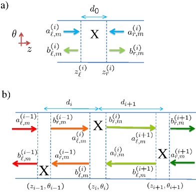
Figure 2: Sketch of input and output amplitudes of the scattering matrix approach for a single impurity (a) and for many impurities (b). In the latter case input and output amplitudes of successive impurities are related.

2.2 Scattering matrix approach

Let us consider a single impurity, the $i$-th one, say, and write the wave function far from it (outside the region of length $d_{0}$, see Fig. 2a) as

$$\psi(z,\theta) = \sum_{m=1}^{M}{a_{c,m}^{(i)}\phi_{m}(\theta)e^{is_{c}k_{m}(z-z_{c}^{(i)})}}$$ (10)

$$+ \sum_{m=1}^{M}{b_{c,m}^{(i)}\phi_{m}(\theta)e^{-is_{c}k_{m}(z-z_{c}^{(i)})}}\;,$$

where $M$ is the number of propagating transverse modes $\{\phi_{m}(\theta)\}$. In Eq. (10) we have introduced a contact label $c=\ell,r$, for left and right asymptotic regions with boundaries at $z_{\ell}^{(i)}$ and $z_{r}^{(i)}$, respectively. We have also defined $s_{\ell}=1$ and $s_{r}=-1$, and the mode wavenumber $k_{m}$ (see the appendix). As it is normally defined datta , the scattering matrix relates output current amplitudes to input ones

$$\left(\begin{array}[]{c}b_{\ell,m}^{(i)}\sqrt{v_{m}}\\ b_{r,m}^{(i)}\sqrt{v_{m}}\end{array}\right)=\left(\begin{array}[]{cc}r_{mn}^{(i)}&{t^{\prime}}_{mn}^{(i)}\\ t_{mn}^{(i)}&{r^{\prime}}_{mn}^{(i)}\\ \end{array}\right)\left(\begin{array}[]{c}a_{\ell,n}^{(i)}\sqrt{v_{n}}\\ a_{r,n}^{(i)}\sqrt{v_{n}}\end{array}\right)\;,$$ (11)

where $v_{m}=\hbar k_{m}/m^{*}$ is the velocity of mode $m$.

Assume now the many impurity scenario of the preceding subsection. As hinted in Fig. 2b, it is clear that input and output amplitudes of successive impurities are related. Indeed,

$$a_{\ell,m}^{(i)} = b_{r,m}^{(i-1)}e^{ik_{m}(d_{i}-d_{0})}\;,$$ (12)

$$a_{r,m}^{(i)} = b_{\ell,m}^{(i+1)}e^{ik_{m}(d_{i+1}-d_{0})}\;.$$ (13)

Notice that the distance between impurities is not a constant, $d_{i}=z_{i}-z_{i-1}$, and that the phases in Eqs. (12) and (13) are due to the different definition of the asymptotic boundaries for each impurity.

Repeatedly using Eqs. (11), (12) and (13) for the successive impurities we would obtain a linear system of equations relating input and output amplitudes of the global disordered region, i.e., between first (leftmost) and ${\cal N}$-th (rightmost) impurities. This total transmission corresponding to, say, unit-amplitude incidence from the left in transverse mode $m_{\rm in}$ to the right in mode $m_{\rm out}$ is simply

$$t_{m_{\rm out}m_{\rm in}}\equiv b^{({\cal N})}_{r,m_{\rm out}}\,\sqrt{\frac{v_{m_{\rm out}}}{v_{m_{\rm in}}}}\;.$$ (14)

The linear system yielding the output $b$-amplitudes reads

$$\left\{\begin{array}[]{rcll}b_{\ell,m}^{(1)}&=&r_{m{m_{\rm in}}}^{(1)}+\displaystyle\sum_{n}{{t^{\prime}}_{mn}^{(1)}\,e^{ik_{n}(d_{2}-d_{0})}\,b_{\ell,n}^{(2)}}&(m=1,\dots,M)\\ \rule{0.0pt}{18.49411pt}b_{r,m}^{(1)}&=&t_{m{m_{\rm in}}}^{(1)}+\displaystyle\sum_{n}{{r^{\prime}}_{mn}^{(1)}\,e^{ik_{n}(d_{2}-d_{0})}\,b_{\ell,n}^{(2)}}&(m=1,\dots,M)\\ \rule{0.0pt}{18.49411pt}b_{\ell,m}^{(i)}&=&\displaystyle\sum_{n}{r_{mn}^{(i)}\,e^{ik_{n}(d_{i}-d_{0})}\,b_{r,n}^{(i-1)}}+\displaystyle\sum_{n}{{t^{\prime}}_{mn}^{(i)}\,e^{ik_{n}(d_{i+1}-d_{0})}\,b_{\ell,n}^{(i+1)}}&(i=2,\dots,{\cal N}-1;m=1,\dots,M)\\ \rule{0.0pt}{18.49411pt}b_{r,m}^{(i)}&=&\displaystyle\sum_{n}{t_{mn}^{(i)}\,e^{ik_{n}(d_{i}-d_{0})}\,b_{r,n}^{(i-1)}}+\displaystyle\sum_{n}{{r^{\prime}}_{mn}^{(i)}\,e^{ik_{n}(d_{i+1}-d_{0})}\,b_{\ell,n}^{(i+1)}}&(i=2,\dots,{\cal N}-1;m=1,\dots,M)\\ \rule{0.0pt}{18.49411pt}b_{\ell,m}^{({\cal N})}&=&\displaystyle\sum_{n}{{r}_{mn}^{({\cal N})}\,e^{ik_{n}(d_{\cal N}-d_{0})}\,b_{r,n}^{({\cal N}-1)}}&(m=1,\dots,M)\\ \rule{0.0pt}{18.49411pt}b_{r,m}^{({\cal N})}&=&\displaystyle\sum_{n}{{t}_{mn}^{({\cal N})}\,e^{ik_{n}(d_{\cal N}-d_{0})}\,b_{r,n}^{({\cal N}-1)}}&(m=1,\dots,M)\end{array}\right.\;.$$ (15)

Equation (15) is a highly sparse linear system of $2M{\cal N}$ equations. It can be very efficiently solved with sparse linear solvers like ME48 of the Harwell library harwell .

As mentioned in the introduction, a major simplifying property derived from the tube symmetry is the transformation relating any two impurities. In fact, defining a reference impurity at $(z_{0},\theta_{0})$ the transmission coefficient for the $i$-th impurity, positioned at $(z_{i},\theta_{i})$, reads

$$t_{mn}^{(i)}=e^{-i(\theta_{i}-\theta_{0})(\lambda_{m}-\lambda_{n})}t_{mn}^{(0)}\;,$$ (16)

where $\lambda_{m}$ is the angular momentum of mode $m$. The phase in Eq. (16) is due to the rotation needed to link the two impurity positions. The longitudinal translation does not introduce any additional phase here because our definition of the scattering matrix implies a translation of the reference boundaries for each impurity. This type of phase does appear however in Eqs. (12) and (13). It can be easily shown that an identical phase to that in Eq. (16) is relating $r_{mn}^{(i)}$, ${t^{\prime}}_{mn}^{(i)}$ and ${r^{\prime}}_{mn}^{(i)}$ with $r_{mn}^{(0)}$, ${t^{\prime}}_{mn}^{(0)}$ and ${r^{\prime}}_{mn}^{(0)}$, respectively. The overall result is that only the reference impurity scattering coefficients are necessary to set up the linear system Eq. (15).

For a given disorder realization we obtain the linear conductance $\tilde{G}$ from Eqs. (15) and (14) using Landauer formula to relate conductance with transmission

$$\tilde{G}=G_{0}\sum_{mn}{|t_{mn}|^{2}}\;.$$ (17)

As well known, Eq. (17) corresponds to a two terminal measurement and it includes the contact resistance, i.e., in absence of any disorder it yields $G=MG_{0}$.

3 Results

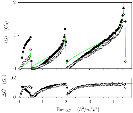
Figure 3: Mean conductance (upper) and variance (lower) for ${\cal N}=1000$ impurities. Solid and open symbols correspond to $d_{1}=0.5\rho$ and $2.5\rho$, respectively. Other parameters we have used are $d_{0}=0.5\rho$ and the impurity potential given by $\sigma=0.05\rho$ and $V_{0}=80\;\hbar^{2}/(m^{*}\rho^{2})$. The solid line in the upper plot corresponds to the semiclassical model and the dash on the right vertical axis of the lower plot gives the universal conductance fluctuation value rev1 .

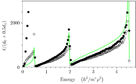
Figure 4: Localization length, scaled by the mean impurity-impurity distance, for the same parameters of Fig. 3. The solid line shows the corresponding semiclassical result for $\alpha^{-1}$.

Figure 3 displays the results obtained for a tube having a fixed number of impurities ${\cal N}=1000$ and an energy range including up to 5 propagating modes. We have fixed $d_{0}=0.5\rho$ and the different symbols are for impurity distributions characterized by $d_{1}=0.5\rho$ (solid) and $d_{1}=2.5\rho$ (open). The mean conductance has a conspicuous sawtooth wave behavior, steadily increasing with energy until a new mode becomes propagating and a sharp drop occurs. The variance, $\Delta\tilde{G}\equiv(\langle\tilde{G}^{2}\rangle-\langle\tilde{G}\rangle^{2})^{1/2}$, shows similar drops and a clear convergence with increasing energy towards the universal conductance fluctuation value. Except for the first plateau plateau the results for $d_{1}=0.5\rho$ and $2.5\rho$ look quite similar.

As mentioned in the introduction, the key to analyze the results of Fig. 3 is the localization length $\ell$. Figure 4 displays this variable for the same parameters of Fig. 3. We have found $\ell$ by disorder averaging the Lyapunov exponent in a long wire. More specifically, we have done the calculations for $10^{4}$ impurities, for which the wire length is much larger than $\ell$ for all energies shown in Fig. 4. There is a qualitative similarity between Figs. 3 and 4. The energy dependence of the conductance for a fixed wire length can be interpreted in terms of the strong variation of the localization length with the energy. In general, as the energy increases the wire evolves from the localized towards the metallic regime until the appearance of a new mode causes a sudden drop back towards the localized case.

The first plateau, with only one propagating mode, shows a qualitative difference from the others. Remarkably, the mean conductance with $1000$ impurities is close to the maximal value $G_{0}$ when $d_{1}=0.5\rho$. For $d_{1}=2.5\rho$ it also shows a different energy dependence with a faster energy increase than for other plateaus. This behavior can be attributed to the effective one dimensionality in this limit. Indeed, it can be shown that the model is equivalent to a Kronig-Penney lattice in which the spacing between 1D barriers is not exactly regular but has some fluctuation around the mean positions. For a fixed $d_{0}$ regularity is inversely proportional to $d_{1}$. The more regular the distribution, the higher the conductance due to the formation of extended Bloch states. This is nicely confirmed by the localization length (Fig. 4) which shows a dramatic enhancement in the first plateau for the smaller $d_{1}$. However, for large enough wire lengths the states are always localized, i.e., $\ell$ is large but remains finite.

It is also worth mentioning that the localization length scales, approximately, with the mean impurity-impurity distance. As Fig. 4 shows, this is clear at the beginning of the second and third plateaus, where a linear increase of the localization length with energy is found. This linear behavior agrees with a prediction discussed by Thouless in Ref. thouless . In this reference the relation between localization length and density of states is stressed, showing that for a particular density of states, a Gaussian white noise model halperin , one finds $\ell\sim E$. The discontinuities in localization length (Fig. 4) could then indicate the existence of discontinuities in the density of states of the disordered system. Such discontinuities would not be surprising since the density of states of the clean quasi-1D system diverges as $(E-\varepsilon_{m})^{-1/2}$ at the beginning of each plateau, when $E\approx\varepsilon_{m}$.

In Fig. 5 we show the probability distributions of the conductance $\tilde{G}$ and Lyapunov exponent $\tilde{\gamma}$ for a fixed energy $E=1.6\hbar^{2}/{(m^{*}\rho^{2})}$ and three different wire lengths, corresponding to 200, 1000 and 5000 impurities and $d_{1}=2.5\rho$. Comparison with the prediction of the theory of disordered conductors, Eqs. (3) and (4), shows the deviation in the intermediate regime, ${\cal N}=1000$, when $L\approx 1.5\ell$ and the wire is neither in localized nor in metallic regime. In the limiting cases, however, either the conductance (metallic) or the Lyapunov exponent (localized) closely follows the expected behavior.

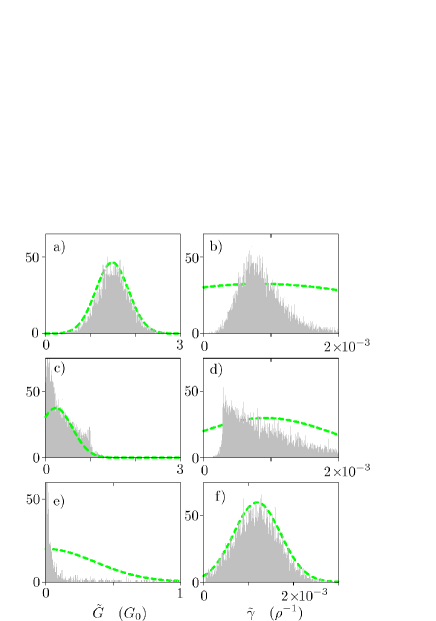
Figure 5: Probability distributions of the conductance (left panels) and Lyapunov exponents (right). Ordered by rows the results correspond to increasing wire lengths: 200 impurities in (a) and (b), 1000 in (c) and (d) and 5000 in (e) and (f). The dashed lines show the normal distributions, Eqs. (3) and (4), from the theory of disordered conductors using an arbitrary vertical scale. As expected, Gaussian distributions are found in the conductance of the metallic regime (a), and in the Lyapunov exponent of the localized regime (f).

Figures 3 and 4 also show the semiclassical result in each case (continuous line). As mentioned in the Introduction, the semiclassical approach neglects interference effects by directly composing the transmission probabilities, as opposed to the phase-coherent composition of transmission amplitudes in fully quantum mechanical calculations. Notice that if all phases of Eqs. (12), (13), (15) and (16) are neglected the formalism does not depend on the impurity positions $(z_{i},\theta_{i})$, only on its total number ${\cal N}$. This causes Ohmic behavior, characterized by parameter $\alpha$ in Eq. (6). It is also possible to relate $\alpha$ with the transmission probability of a single impurity $T^{(1)}$. Indeed, using the composition rule of incoherent scatterers we find the total transmission $T$ from

$$\frac{1}{T}-\frac{1}{M}={\cal N}\left(\frac{1}{T^{(1)}}-\frac{1}{M}\right)\;,$$ (18)

leading to the explicit expression

$$\alpha=\left(\frac{1}{T^{(1)}}-\frac{1}{M}\right)\frac{1}{d_{0}+0.5d_{1}}\;.$$ (19)

As seen in Fig. 4, $\alpha^{-1}$ is close to the localization length or, equivalently, $\alpha$ is close to the Lyapunov exponent. However, both values do not coincide in general, making the comparison between quantum and classical conductance, Eq. (7), rather involved. Another information we can extract from the semiclassical result regards the discontinuities in localization length as a function of energy. Besides Thouless’ argument on the density of states given above, we also expect similar drops in the semiclassical length $\alpha^{-1}$ from Eq. (19). Indeed, the dependence of $T^{(1)}$ on energy is a staircase with rounded edges. This smooth energy dependence is broken by the explicit appearance of $M$, the number of modes, in Eq. (19). A sharp increase in $\alpha$ occurs when the energy allows a new mode but $T^{(1)}$ has not yet increased.

4 Conclusions

We have studied the quantum transport properties of tubular shaped nanowires with randomly distributed impurities. For a given wire length our calculations predict a sawtooth-like behavior of the conductance as a function of energy; conspicuous drops appearing when the energy is just barely enough to allow the propagation of a new transverse mode. The analysis of our results within the scaling theory of disordered conductors explains the observed behavior as a general tendency of the wire to evolve from localized towards metallic regimes with increasing energy. Abrupt changes in the density of states occur when a new mode becomes propagating, leading the wire back towards a more localized regime.

We have also calculated the localization length of the disordered wire for energies covering from one to five propagating modes. Qualitative interpretation in terms of the density of states explains the linear-with-energy dependence at the beginning of the conducting plateaus, as well as the discontinuous drops already mentioned. The semiclassical description has been also discussed and shown to provide a complementary interpretation of the discontinuous drops. In the metallic regime, the comparison between the average quantum conductance and the semiclassical one is complicated when the Lyapunov exponent and the semiclassical coefficient for Ohmic behavior do not coincide.

Appendix A Single impurity scattering

The formalism of Sec. 2.2 requires the scattering matrix of a single impurity as an input. We find this by solving the Schrödinger equation for the corresponding open boundary problem using the quantum-transmitting boundary algorithm qtbm . The wave function fulfills the equation

$$\left(-\frac{\hbar^{2}}{2m^{*}}\frac{d^{2}}{dz^{2}}-\frac{\hbar^{2}}{2m^{*}\rho^{2}}\frac{d^{2}}{d\theta^{2}}+V(z,\theta)\right) \psi(z,\theta) =$$

$$E \psi(z,\theta) \;,$$ (20)

where $m^{*}$ is the electron’s effective mass and $V(z,\theta)$ is given by Eq. (8) with the impurity at $(z_{i},\theta_{i})=(0,0)$. Far from the impurity, in the parts of the tube that play the role of contact leads (or contacts for short), the potential vanishes and the Hamiltonian separates in longitudinal and angular (transverse) contributions. The angular problem

$$-\frac{\hbar^{2}}{2m^{*}\rho^{2}}\frac{d^{2}\phi_{n}(\theta)}{d\theta^{2}}=\varepsilon_{n}\phi_{n}(\theta)\;,$$ (21)

yields the set of transverse modes $\{\phi_{n},\varepsilon_{n}\}$,

$$\phi_{n}(\theta) = \frac{1}{\sqrt{2\pi}}e^{i\lambda_{n}\theta}\quad(\lambda_{n}=0,\pm 1,\dots)\;,$$ (22)

$$\varepsilon_{n} = \frac{\hbar^{2}\lambda_{n}^{2}}{2m^{*}\rho^{2}}\;.$$ (23)

Equation (A) can be solved using finite differences in a Cartesian grid. However, increasing the number of grid points becomes very costly and this method lacks accuracy in the angular integrations with oscillating functions like those of Eq. (22). Therefore, we have used a mixed approach, in which the $z$ coordinate is discretized in a uniform grid while the angular dependence is described by expanding in the angular eigenfunctions, i.e.,

$$\psi(z,\theta)=\sum_{n}{\psi_{n}(z)\,\phi_{n}(\theta)}\;.$$ (24)

The unknown band amplitudes $\psi_{n}(z)$ fulfill coupled-channel equations

$$-\frac{\hbar^{2}}{2m^{*}}\psi_{n}^{{}^{\prime\prime}}(z)+(\varepsilon_{n}-E)\,\psi_{n}(z)=-\sum_{n^{\prime}}{V_{nn^{\prime}}(z)\psi_{n^{\prime}}(z)}\;,$$ (25)

where

$$V_{nn^{\prime}}(z)=\frac{1}{2\pi}\int{d\theta\,V(z,\theta)e^{i(\lambda_{n}-\lambda_{n^{\prime}})\theta}}\;.$$ (26)

In the contacts the band amplitudes take a similar form to Eq. (10),

$$\psi_{n}(z)=a_{c,n}e^{is_{c}k_{n}(z-z_{c})}+b_{c,n}e^{-is_{c}k_{n}(z-z_{c})}\;.$$ (27)

This expression is for a propagating channel, for which $\varepsilon_{n}<E$ and $k_{n}=\sqrt{2m^{*}(E-\varepsilon_{n})}/\hbar$ is a real number. It also applies to evanescent ones, $\varepsilon_{n}>E$, if we assume in this case $a_{c,n}=0$ and a purely imaginary wavenumber $k_{n}=i\sqrt{2m^{*}(\varepsilon_{n}-E)}/\hbar$. Notice that the output amplitudes can be obtained from the wave function right at the contact position,

$$b_{c,n}=\psi_{n}(z_{c})-a_{c,n}\;.$$ (28)

Substituting Eq. (28) in Eq. (27) we obtain

$$\psi_{n}(z)-\psi_{n}(z_{c})\,e^{-is_{c}k_{n}(z-z_{c})}=$$

$$2ia_{c,n}\sin \!\!\!(s_{c}k_{n}(z-z_{c}))\,,$$ (29)

which is the quantum-transmitting-boundary equation for the contacts.

Equations (25) and (A), for the central and contact regions, respectively, form a closed set which does not invoke the wave function at any external point. Of course, this is not true for any of these two subsets separately, since central and contact regions are connected through the derivative in Eq. (25) and of $\psi_{n}(z_{c})$ in Eq. (A). In practice, we use a uniform grid in $z$ with $n$-point formulae for the derivatives ($n\approx 5-11$) and truncate the expansion in transverse bands, Eq. (24), to include typically 50-100 terms. The resulting sparse linear problem is then solved as in Sec. 2.2 using routine ME48 harwell .

References

- (1) P.W. Anderson, Phys. Rev. 109, 1492 (1958)
- (2) P.W. Anderson, D.J. Thouless, E. Abrahams, D.S. Fisher, Phys. Rev. B 22, 3519 (1980)
- (3) C.W.J. Beenakker, Rev. Mod. Phys. 69, 731 (1997)
- (4) L.I. Deych, A.A. Lisyansky, and B.L. Altshuler, Phys. Rev. B 64, 224202 (2001)
- (5) J.B. Pendry, Advances in Physics 43, 461 (1994)
- (6) B. Kramer and A. MacKinnon, Rep. Prog. Phys. 56, 1469 (1993).
- (7) V.Y. Prinz, V.A. Seleznev, A.K. Gutakovsky, A.V. Chehovskiy, V.V. Preobrazhenskii, M.A. Putyato, and T.A. Gavrilova, Physica E 6, 828 (2000)
- (8) O.G. Schmidt and K. Eberl, Nature (London) 410, 168 (2001)
- (9) A. Lorke, S. Böhm, and W. Wegscheider, Superlattices Microstruct. 33, 347 (2003)
- (10) N. Shaji, H. Qin, R.H. Blick, L.J. Klein, C. Deneke, and O.G. Schmidt, Appl. Phys. Lett. 90, 042101 (2007)
- (11) M. Jung, J.S. Lee, W. Song, Y.H. Kim, S.D. Lee, N. Kim, J. Park, M.-S. Choi, S. Katsumoto, H. Lee, J. Kim, Nanoletters 8, 3189 (2008)
- (12) G. Ferrari, A. Bertoni, G. Goldoni, and E. Molinari Phys. Rev. B 78, 115326 (2008)
- (13) M. Trushin and J. Schliemann, New Journal of Physics 9, 346 (2007)
- (14) L.I. Magarill, D.A. Romanov, A.V. Chaplik, JETP 86, 771 (1998)
- (15) M. Cahay, M. McLennan, S. Datta, Phys. Rev. B 37, 10125 (1988)
- (16) This result, discussed at the end of Sec. 3, is exactly fulfilled in the tube symmetry. It is not evident in other geometries like the planar one (see Ref. cahay )
- (17) D.J. Thouless, J. Phys. C 5, 77 (1972)
- (18) S. Datta, Electronic transport in mesoscopic systems (Cambridge University Press, 1997)
- (19) HSL, A Collection of Fortran codes for large-scale scientific computation. See http://www.hsl.rl.ac.uk, (2007)
- (20) Although the energy dependence of the conductance with disorder no longer resembles a staircase we still refer by plateaus to the different energy intervals in which the number of modes is constant. For instance, the first plateau, with just one mode, corresponds to .
- (21) B.I. Halperin, Phys. Rev. 139, A104 (1965)
- (22) C.S. Lent, D.J. Kirkner, J. Appl. Phys. 67, 6353 (1990)