Parameter estimation for coalescing massive binary black holes with LISA using the full 2-post-Newtonian gravitational waveform and spin-orbit precession

Abstract

Gravitational waves emitted by binary systems in the inspiral phase carry a complicated structure, consisting in a superposition of different harmonics of the orbital frequency, the amplitude of each of them taking the form of a post-Newtonian series. In addition to that, spinning binaries experience spin-orbit and spin-spin couplings which induce a precession of the orbital angular momentum and of the individual spins. With one exception, previous analyses of the measurement accuracy of gravitational wave experiments for comparable-mass binary systems have neglected either spin-precession effects or subdominant harmonics and amplitude modulations. Here we give the first explicit description of how these effects combine to improve parameter estimation. We consider supermassive black hole binaries as expected to be observed with the planned space-based interferometer LISA, and study the measurement accuracy for several astrophysically interesting parameters obtainable taking into account the full 2PN waveform for spinning bodies, as well as spin-precession effects. We find that for binaries with a total mass in the range $10^{5}M_{\odot}<M<10^{7}M_{\odot}$ at a redshift of $1$, a factor $\sim 1.5$ is in general gained in accuracy, with the notable exception of the determination of the individual masses in equal-mass systems, for which a factor $\sim 5$ can be gained. We also find, as could be expected, that using the full waveform helps increasing the upper mass limit for detection, which can be as high as $M=10^{8}M_{\odot}$ at a redshift of 1, as well as the redshift limit where some information can be extracted from a system, which is roughly $z\gtrsim 10$ for $M\leqslant 10^{7}M_{\odot}$, $1.5\ \mbox{-}\ 5$ times higher than with the restricted waveform. We computed that the full waveform allows to use supermassive black hole binaries as standard sirens up to a redshift of $z\approx 1.6$, about $0.4$ larger than what previous studies allowed. We found that for lower unequal-mass binary systems, the measurement accuracy is not as drastically improved as for other systems. This suggests that for these systems, adding parameters such as eccentricity or alternative gravity parameters could be achieved without much loss in the accuracy.

I Introduction

Gravitational waves (GW’s), once their observation is made possible, will provide new means of observing the Universe. So far, the vast majority of observations have been made through electromagnetic radiation, and gravitational waves will surely make visible different aspects of the Universe. For example, one could probe the different galaxy formation models by detecting supermassive black hole mergers in a large redshift range Sesana et al. (2007). Or, as GW’s provide a good way of measuring the luminosity distance to their source, one could combine gravitational and electromagnetic observations to build a robust measurement of the Hubble diagram, which would be of great interest for cosmology Schutz (1986); Holz and Hughes (2005). Another possibility would be to measure alternative gravity parameters Berti et al. (2005); Arun and Will (2009); Stavridis and Will (2009). This can potentially be a powerful way to constrain such theories, as each observed GW will give an independent measurement of their parameters.

The new generation of ground-based detectors, such as advanced LIGO, and the space-based detector LISA will probably make the direct detection of gravitational waves possible. Some of the most important sources of gravitational waves are the compact binary systems, i.e. systems of two compact objects (white dwarfs, neutron stars, or black holes). As such detections rely on matched filtering techniques, several groups have made efforts in building accurate templates based on the post-Newtonian (PN) approximation (see e.g. Thorne and Hartle (1985); Owen et al. (1998); Faye et al. (2006); Blanchet et al. (2006); Arun et al. (2004, 2009a)). The limitations of such results have then been checked to estimate the precision with which one could measure the properties of a system emitting such waves, for example its distance from the Solar System, location in the sky, or the individual masses of the objects forming it Finn (1992); Cutler (1998); Hughes (2002); Vecchio (2004); Lang and Hughes (2006); Arun et al. (2007); Porter and Cornish (2008); Trias and Sintes (2008).

A binary system of compact objects emits gravitational waves during three distinct phases, called inspiral, merger, and ringdown. During the inspiral phase, most of the gravitational radiation is emitted at twice the orbital frequency of the system, which slowly increases as it loses energy emitting gravitational waves. As its two members come closer, higher harmonics become more and more important, and more power gets emitted. Finally, the two members enter the merger phase, where they have come so close that they cannot be treated anymore as two separate objects, and begin to merge, emitting complicated gravitational radiation that has not yet been described but numerically. After that, the remnant begins to radiate away its energy during the ringdown phase, where it approaches exponentially the structure of a Kerr black hole.

LISA has been designed to be particularly sensitive to binaries that contain a supermassive black hole (SMBH, of mass $10^{5}\ \mbox{-}\ 10^{8}M_{\odot}$), which can be separated into two (or three) categories, according to the companion mass: extreme mass-ratio inspirals (EMRIs) and supermassive black hole binaries (SMBHBs). A third category is sometimes added: intermediate mass ratio inspirals (IMRIs), which somehow lies between the two others.

EMRIs are inspirals with a mass ratio between the two members of the order of $10^{-4}\ \mbox{-}\ 10^{-7}$, and are most accurately described by black hole perturbation theory. Such events are likely to occur in the center of galaxies, the majority of which are believed to host a SMBH, when a compact object of stellar mass is “eaten up” by the central object. Several groups have attacked the problem of describing the form of the gravitational radiation emitted by such objects Cutler et al. (1994); Barack and Cutler (2004); Babak et al. (2007).

SMBHBs are binaries containing two SMBHs, forming during the merging of two galaxies, when they both host one in their center. Such events should be much more rare than EMRIs, but some galaxy formation models Berti (2006) and observation of nearby galaxies Narayan (2005) suggest that they might happen often enough to be observable. As these events are much louder than any other source, we could observe them at very high redshifts (up to $z=20$ or even higher), and thus tightly constrain galaxy formation models.

The first attempt to estimate with which accuracy an interferometer could measure the properties of a compact object binary was made by Finn Finn (1992), who first introduced the Fisher matrix analysis, which is now widely used in this context. A few years later, Cutler Cutler (1998) applied this formalism to LISA, focusing on the angular resolution that the space-based detector could get for black hole binaries, using the Newtonian quadrupole formula. Hughes Hughes (2002) repeated the study including the PN expansion for the frequency of the wave. Vecchio Vecchio (2004), then, considered the case of the “simple precession” Apostolatos et al. (1994) of the angular momenta for spinning BH’s. Lang and Hughes Lang and Hughes (2006) then used the full precession equations to further refine the parameter estimation. Recently, Arun et al. Arun et al. (2007) and Porter and Cornish Porter and Cornish (2008) included the full post-Newtonian waveform in the context of nonspinning black holes, and Trias and Sintes Trias and Sintes (2008) used it for spinning black holes neglecting spin-precession effects. The LISA Parameter Estimation Taskforce Arun et al. (2009b) used the full waveform with spin-precession effects, without publishing a detailed study of the expected statistical errors. It is worth noting that all of the effects that these works studied, as more and more precise waveforms were used, helped to improve subsequently the expected measurement accuracy of LISA. In this paper, we study the question of whether the inclusion of the full post-Newtonian waveform in the context of spinning black holes undergoing spin-orbit precession helps to break more degeneracies, thus helping to further increase the accuracy in the measurement of the source parameters.

In Sec. II, we derive the waveform used to perform our study, and we quote some basics of Fisher matrix analysis. In Sec. III, we describe the simulations that we ran. In Sec. IV, we give the results of our simulations, and analyze them from an astrophysical point of view. We conclude in Sec. V.

II Theory

II.1 Evolution

The state of a binary system of two Kerr black holes at a given time in the center of mass frame is fully described by 14 intrinsic parameters. These reduce to 12 if we assume that the binary lies on a circular orbit. One possible choice is to take as intrinsic parameters a unit vector pointing in the direction of the orbital angular momentum $\bm{\hat{L}}$, the orbital angular frequency $\omega$ (we will reserve the symbol $f$ for arguments of Fourier transforms, and will express the orbital frequency always with the angular frequency to avoid confusions), the individual spins of each black hole, $\bm{S}_{1}$ and $\bm{S}_{2}$, their masses $m_{1}$ and $m_{2}$, and the orbital phase $\varphi$. To these intrinsic parameters, we have to add three more extrinsic parameters which locate the binary in space. Those can be chosen to be $\bm{\hat{n}}$, a unit vector pointing in the direction of the binary as seen from the Solar System, and $d_{L}$, the luminosity distance from the binary to the Sun. We will denote all unit vectors with a hat throughout this paper.

Another extrinsic parameter, the redshift, also plays a role in the determination of the waveform, but it cannot be detected by GW observations. Indeed, the redshift causes the observed angular frequency $f_{o}$ of the wave to decrease with respect to the emitted one $f_{e}$, as $f_{o}=f_{e}/(1+z)$. But (see following derivation) the exact same wave, within the post-Newtonian framework, is emitted by a second system with parameters $m_{i}^{(2)}=(1+z)m_{i}^{(1)}$, $d_{L}^{(2)}=(1+z)d_{L}^{(1)}$, not experiencing any redshift. Therefore, the redshift and luminosity distance cannot be measured separately with a gravitational wave observation, so that we have to assume a relation between the two parameters. This implies that observations of a light signal emitted during a merger, the redshift of which is possible to determine, are of great astrophysical interest. During the whole derivation of the gravitational wave signal below, we assume that the source is at redshift $z=0$. The actual observed wave can then be easily determined redshifting the masses and luminosity distance, as we did in our simulations.

To compute the relation between redshift and luminosity distance, we assume a flat $\Lambda$CDM cosmology without radiation with the latest WMAP parameters Komatsu et al. (2009): $\Omega_{\Lambda}=0.72$, $\Omega_{m}=0.28$, $H_{0}=70.1$ km/s/Mpc.

The relation is then given by

$$d_{L}(z)=(1+z)\frac{c}{H_{0}}\int_{0}^{z}\frac{dz^{\prime}}{\sqrt{\Omega_{m}(1+z^{\prime})^{3}+\Omega_{\Lambda}}},$$ (1)

which can be determined numerically.

The problem of the motion of the system during the inspiral phase in full General Relativity has been too hard to be solved so far. However, a great effort has been made to attack the problem in the framework of the post-Newtonian formalism. The current state-of-the-art evolution equations go up to the 2.5PN order beyond leading order for spinning objects Faye et al. (2006). As 2.5PN spin-orbit and spin-spin coupling terms are not yet known in the waveform, we chose to stop at the 2PN level, up to which both the evolution equations and the waveform are known. We will use the following mass parameters for the derivation of the evolution equations and of the waveform: the total mass $M=m_{1}+m_{2}$, the reduced mass $\mu=m_{1}m_{2}/M$, and the symmetric mass ratio $\nu=\mu/M$.

The 2PN orbit-averaged relation between the orbital angular frequency $\omega$ and the orbital separation in harmonic coordinates $r$ is given by Blanchet et al. (2006)

$$\omega=\frac{c^{3}}{GM}\gamma^{3/2}\bigg{[}1+\left(\frac{\nu}{2}-\frac{3}{2}\right)\gamma-\frac{1}{2}\beta(2,3)\gamma^{3/2}\\ +\left(\frac{15}{8}+\frac{47\nu}{8}+\frac{3\nu^{2}}{8}-\frac{3}{4}\sigma(1,3)\right)\gamma^{2}\bigg{]},$$ (2)

where the orbital separation parameter $\gamma$ and the spin-orbit and spin-spin couplings $\beta$ and $\sigma$ are given by

$$\gamma \equiv\frac{GM}{rc^{2}},$$ (3)

$$\beta(a,b) \equiv\frac{c}{G}\sum_{i=1}^{2}\left(\frac{a}{M^{2}}+\frac{b\nu}{m_{i}^{\phantom{i}2}}\right)\bm{S}_{i}\cdot\bm{\hat{L}},$$ (4)

$$\sigma(a,b) \equiv\frac{c^{2}}{\nu M^{4}G^{2}}\left(a\bm{S}_{1}\cdot\bm{S}_{2}-b\left(\bm{S}_{1}\cdot\bm{\hat{L}}\right)\left(\bm{S}_{2}\cdot\bm{\hat{L}}\right)\right).$$ (5)

The evolution equation of the angular frequency is given at 2PN order by Blanchet et al. (2006)

$$\frac{dx}{dt} =\frac{64\nu}{5}\frac{c^{3}}{GM}x^{5}\Bigg{[}1-\left(\frac{743}{336}+\frac{11\nu}{4}\right)x$$

$$+\left(4\pi-\frac{1}{12}\beta(113,75)\right)x^{3/2}$$ (6)

$$+\left(\frac{34103}{18144}+\frac{13661\nu}{2016}+\frac{59\nu^{2}}{18}-\frac{1}{48}\sigma(247,721)\right)x^{2}\Bigg{]},$$

where $x$ is a dimensionless orbital frequency parameter defined as

$$x\equiv\left(\frac{GM\omega}{c^{3}}\right)^{2/3}.$$ (7)

We can integrate Eq. (6) to get

$$t =t_{c}-\frac{5GM}{256\nu c^{3}}x^{-4}\bigg{[}1+\left(\frac{743}{252}+\frac{11\nu}{3}\right)x$$

$$+\left(\frac{2}{15}\beta(113,75)-\frac{32}{5}\pi\right)x^{3/2}$$ (8)

$$+\left(\frac{3058673}{508032}+\frac{5429\nu}{504}+\frac{617\nu^{2}}{72}+\frac{1}{24}\sigma(247,721)\right)x^{2}\bigg{]}.$$

Integrating once more yields the orbital phase $\varphi=\int\omega dt$, as a function of the orbital frequency parameter

$$\varphi(x) =\varphi_{c}-\frac{x^{-5/2}}{32\nu}\bigg{[}1+\left(\frac{3715}{1008}+\frac{55\nu}{12}\right)x$$

$$\phantom{=}+\left(\frac{5}{24}\beta(113,75)-10\pi\right)x^{3/2}$$

$$\phantom{=}+\bigg{(}\frac{15293365}{1016064}+\frac{27145\nu}{1008}$$

$$\phantom{=}+\frac{3085\nu^{2}}{144}+\frac{5}{48}\sigma(247,721)\bigg{)}x^{2}\bigg{]}.$$ (9)

The dragging of inertial frames induces a coupling between the individual spins and the orbital angular momentum. The orbit-averaged conservative part of the evolution equations (i.e. without radiation reaction, $\dot{\bm{L}}+\dot{\bm{S}}_{1}+\dot{\bm{S}}_{2}=0$) are given for circular orbits at 2PN order by

$$\dot{\bm{L}} =\frac{G}{c^{2}}\frac{1}{r^{3}}\left(\left(2+\frac{3m_{2}}{2m_{1}}\right)\bm{S}_{1}+\left(2+\frac{3m_{1}}{2m_{2}}\right)\bm{S}_{2}\right)\times\bm{L}$$

$$\phantom{=}-\frac{3G}{2c^{2}}\frac{1}{r^{3}}\left(\left(\bm{S}_{2}\cdot\bm{\hat{L}}\right)\bm{S}_{1}+\left(\bm{S}_{1}\cdot\bm{\hat{L}}\right)\bm{S}_{2}\right)\times\bm{\hat{L}},$$ (10)

$$\dot{\bm{S}}_{i} =\frac{G}{c^{2}}\frac{1}{r^{3}}\left[\left(2+\frac{3m_{j}}{2m_{i}}\right)\bm{L}+\frac{1}{2}\bm{S}_{j}-\frac{3}{2}\left(\bm{S}_{j}\cdot\bm{\hat{L}}\right)\bm{\hat{L}}\right]\times\bm{S}_{i},$$ (11)

where it is understood that $i\neq j$, $i,j\in\{1,2\}$, and the orbital separation $r$ and the norm of the orbital angular momentum $L$ are related to the orbital frequency by their Newtonian relation:

$$L =\mu\left(\frac{G^{2}M^{2}}{\omega}\right)^{1/3},$$ (12)

$$r =\left(\frac{GM}{\omega^{2}}\right)^{1/3}.$$ (13)

Higher order relations would give corrections which exceed the 2PN order.

Using the above relations together with the first order of Eq. (6), we can change variables from time to orbital angular frequency, and use the relations to express the precession equations:

$$\frac{d\bm{S}_{i}}{d\omega} =\frac{5}{96}\frac{c^{3}}{GM}\omega^{-2}\Bigg{[}\bm{\hat{L}}\times\bm{\Sigma}_{i}$$

$$+\frac{1}{2L}\left(\bm{S}_{j}-3\left(\bm{S}_{j}\cdot\bm{\hat{L}}\right)\bm{\hat{L}}\right)\times\bm{S}_{i}\Bigg{]},$$ (14)

$$\frac{d\bm{\hat{L}}}{d\omega} =\frac{5}{96}\frac{c^{3}}{GM}\omega^{-2}\frac{1}{L}\left[\bm{\Sigma}_{1}+\bm{\Sigma}_{2}-\frac{3}{2L}\left(\bm{\sigma}_{1}+\bm{\sigma}_{2}\right)\right]\times\bm{\hat{L}}$$ (15)

$$=-\frac{1}{L}\left(\frac{d\bm{S}_{1}}{d\omega}+\frac{d\bm{S}_{2}}{d\omega}\right),$$

where

$$\bm{\Sigma}_{i} =\left(2+\frac{3m_{j}}{2m_{i}}\right)\bm{S}_{i},$$ (16)

$$\bm{\sigma}_{i} =\left(\bm{S}_{j}\cdot\bm{\hat{L}}\right)\bm{S}_{i}.$$ (17)

II.2 Waveform

The general form of a gravitational wave emitted by a two-body system, even nonspinning, is not known in the context of full general relativity. However, it has been computed in the post-Newtonian framework. The results for a nonspinning binary system are available at 2.5PN order Arun et al. (2004), and the spin effects at 2PN order Arun et al. (2009a).

A convenient way to define the phase of the wave observed in a detector is in terms of the “principal+ direction” Apostolatos et al. (1994), which is defined as the direction of the vector $\bm{\hat{L}}\times\bm{\hat{n}}$. As the orbital angular momentum precesses, the principal+ direction changes, and this must be taken into account in the waveform. This effect amounts, at 2PN order, to

$$\delta\varphi =-\int_{t}^{t_{c}}\frac{\bm{\hat{L}}\cdot\bm{\hat{n}}}{1-\left(\bm{\hat{L}}\cdot\bm{\hat{n}}\right)^{2}}\left(\bm{\hat{L}}\times\bm{\hat{n}}\right)\cdot\dot{\bm{\hat{L}}}dt$$

$$=\delta\varphi_{0}+\int_{\omega_{0}}^{\omega}\frac{\bm{\hat{L}}\cdot\bm{\hat{n}}}{1-\left(\bm{\hat{L}}\cdot\bm{\hat{n}}\right)^{2}}\left(\bm{\hat{L}}\times\bm{\hat{n}}\right)\cdot\frac{d\bm{\hat{L}}}{d\omega}d\omega,$$ (18)

where $\omega_{0}$ is an arbitrary constant corresponding to the time $t_{0}$, $\delta\varphi_{0}=-\int_{t_{0}}^{t_{c}}(d\delta\varphi/dt)dt$, and $d\bm{\hat{L}}/d\omega$ is given in Eq. (15).

The 2PN accurate orbital phase is then given in terms of orbital angular frequency by: $\phi(\omega)=\varphi(\omega)+\delta\varphi(\omega)$.

The waveform is a series of harmonics of the orbital frequency:

$$h_{+,\times}=\frac{2GM\nu x}{d_{L}c^{2}}\left[\sum_{n\geqslant 0}\left(A_{+,\times}^{(n)}\cos n\phi+B_{+,\times}^{(n)}\sin n\phi\right)\right].$$ (19)

The coefficients of the series take the form of post-Newtonian series:

$$A_{+,\times}^{(n)}=\sum_{i\geqslant 0}a^{(n,i/2)}_{+,\times}x^{i/2},$$ (20)

$$B_{+,\times}^{(n)}=\sum_{i\geqslant 0}b^{(n,i/2)}_{+,\times}x^{i/2}.$$ (21)

The exact form of the coefficients for a nonspinning system can be found in Arun et al. (2004, 2009a). Note, however, that both express their final result using another phase which differs from the orbital phase at 1.5PN order: $\Psi=\phi-2\log(\omega/\bar{\omega})x^{3/2}$, where $\bar{\omega}$ is an arbitrary constant. We put together the results from these two papers to build a coherent 2PN accurate waveform for spinning bodies, see the appendix.

II.2.1 Extrinsic effects

The LISA constellation will consist in three spacecrafts launched in orbit around the Sun, at a mean distance of 1 AU, on slightly eccentric orbit so that the spacecrafts stay at the same distance from each other all along the year. The barycenter of LISA will be located on the orbit of the Earth, 20^∘ behind it, and the normal to the plane on which the spacecrafts lie will make a 60^∘ angle with the normal to the ecliptic, see Fig. 1.

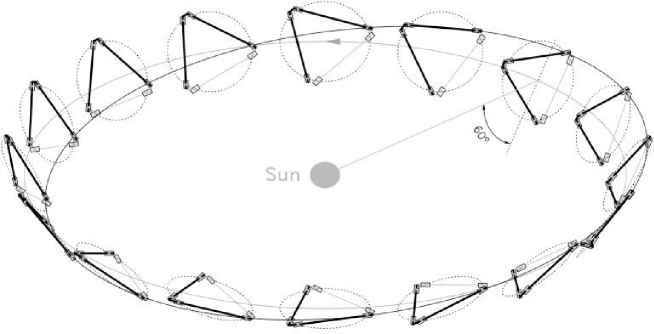
Figure 1: The orbit of LISA around the Sun as currently planned. Image taken from the LISA pre-phase-A report Danzmann et al. (1996).

To describe extrinsic effects that depend on the position of LISA, we follow Cutler (1998) and define two different frames: a frame tied to the detector, $(x,y,z)$, and a fixed, Solar System frame, tied to the distant stars $(\bar{x},\bar{y},\bar{z})$ (we consider that the motion of the Sun with respect to the distant stars can be neglected during the lifetime of the LISA mission).

The unit vectors along the arms of LISA $\bm{\hat{l}}_{i}$, $i\in\{1,2,3\}$ are defined in the detector frame:

$$\bm{\hat{l}}_{i} =\cos\gamma_{i}\bm{\hat{x}}+\sin\gamma_{i}\bm{\hat{y}},$$

$$\gamma_{i} =\frac{\pi}{12}+(i-1)\frac{\pi}{3}.$$ (22)

The $(\bar{x},\bar{y})$ plane of the Solar System frame is defined to be the ecliptic, so that the spherical angles of the barycenter of LISA are

$$\bar{\Theta}=\frac{\pi}{2},\qquad\bar{\Phi}(t)=2\pi t/T,$$ (23)

where $T=1$ yr, and we chose that $\bar{\Phi}=0$ at $t=0$.

The waveform is given relative to the Solar System frame. To take into account the fact that the detector is not static in this frame, we have to add a phase to each harmonic, which is equivalent to add the so-called Doppler phase to the orbital phase:

$$\phi_{D}(t)=\frac{\omega R}{c}\sin\bar{\theta}_{N}\cos(\bar{\Phi}(t)-\bar{\phi}_{N}),$$ (24)

where $R=1$ AU, and $\bar{\theta}_{N}$ and $\bar{\phi}_{N}$ are the spherical angles of the position of the source in the Solar System frame.

The orbital phase then becomes

$$\psi=\phi+\phi_{D}=\varphi+\delta\varphi+\phi_{D}$$ (25)

The normal to the detector plane $\bm{\hat{z}}$ is at constant angle $\bar{\theta}_{z}=\pi/3$ from the normal to the ecliptic $\bm{\hat{\bar{z}}}$, and constantly points in the direction of the $\bar{z}$-axis from the barycenter of LISA. Furthermore, each satellite rotates around the $\bm{\hat{z}}$-axis once a year (see Fig. 1). Let us express then the detector frame in the Solar System frame, assuming that $\bm{\hat{y}}\cdot\bm{\hat{\bar{y}}}=1$ at $t=0$:

$$\bm{\hat{x}} =\left(\frac{3}{4}-\frac{1}{4}\cos 2\bar{\Phi}(t)\right)\bm{\hat{\bar{x}}}-\frac{1}{4}\sin 2\bar{\Phi}(t)\bm{\hat{\bar{y}}}$$

$$\qquad\qquad\qquad\qquad\qquad+\frac{\sqrt{3}}{2}\cos\bar{\Phi}(t)\bm{\hat{\bar{z}}},$$ (26)

$$\bm{\hat{y}} =-\frac{1}{4}\sin 2\bar{\Phi}(t)\bm{\hat{\bar{x}}}+\left(\frac{3}{4}+\frac{1}{4}\cos 2\bar{\Phi}(t)\right)\bm{\hat{\bar{y}}}$$

$$\qquad\qquad\qquad\qquad\qquad+\frac{\sqrt{3}}{2}\sin\bar{\Phi}(t)\bm{\hat{\bar{z}}},$$ (27)

$$\bm{\hat{z}} =-\frac{\sqrt{3}}{2}\cos\bar{\Phi}(t)\bm{\hat{\bar{x}}}-\frac{\sqrt{3}}{2}\sin\bar{\Phi}(t)\bm{\hat{\bar{y}}}+\frac{1}{2}\bm{\hat{\bar{z}}}.$$ (28)

LISA will act during the incoming of a gravitational wave as a pair of two-arm detectors, but with a response scaled by a $\sqrt{3}/2$ factor due to the $60^{\circ}$ opening angle of the constellation, following the pattern ($k=1,2$):

$$h_{k} =\frac{\sqrt{3}}{2}\left(F_{k}^{+}h_{+}+F_{k}^{\times}h_{\times}\right),$$ (29)

$$F_{1}^{+}(\theta_{N},\phi_{N},\psi_{N}) =\frac{1}{2}\left(1+\cos^{2}\theta_{N}\right)\cos 2\phi_{N}\cos 2\psi_{N}$$

$$\phantom{=}-\cos\theta_{N}\sin 2\phi_{N}\sin 2\psi_{N},$$ (30)

$$F_{1}^{\times}(\theta_{N},\phi_{N},\psi_{N}) =F_{1}^{+}(\theta_{N},\phi_{N},\psi_{N}-\pi/4),$$ (31)

$$F_{2}^{+}(\theta_{N},\phi_{N},\psi_{N}) =F_{1}^{+}(\theta_{N},\phi_{N}-\pi/4,\psi_{N}),$$ (32)

$$F_{2}^{\times}(\theta_{N},\phi_{N},\psi_{N}) =F_{1}^{+}(\theta_{N},\phi_{N}-\pi/4,\psi_{N}-\pi/4),$$ (33)

where $\theta_{N}$ and $\phi_{N}$ are the spherical angles of the position of the binary in the detector frame, and $\psi_{N}$ is defined through

$$\tan\psi_{N}\equiv\frac{\bm{\hat{L}}\cdot\bm{\hat{z}}-(\bm{\hat{L}}\cdot\bm{\hat{n}})(\bm{\hat{z}}\cdot\bm{\hat{n}})}{\bm{\hat{n}}\cdot(\bm{\hat{L}}\times\bm{\hat{z}})}.$$ (34)

We expressed here two combinations of the response of the three arms of LISA whose detector noises are uncorrelated Cutler (1998).

Using this, we find the response function of the detectors ($k=1,2$):

$$h_{k} =\frac{\sqrt{3}GM\nu x}{d_{L}c^{2}}\sum_{n\geqslant 0}\Bigg{[}$$

$$\phantom{=}\sum_{i\geqslant 0}\left(F_{k}^{+}(t)a_{+}^{(n,i/2)}+F_{k}^{\times}(t)a_{\times}^{(n,i/2)}\right)x^{i/2}\cos n\psi$$

$$\phantom{=}+\sum_{i\geqslant 0}\left(F_{k}^{+}(t)b_{+}^{(n,i/2)}+F_{k}^{\times}(t)b_{\times}^{(n,i/2)}\right)x^{i/2}\sin n\psi\Bigg{]}$$ (35)

$$=\frac{\sqrt{3}GM\nu x}{d_{L}c^{2}}\sum_{n\geq 0}\left[A_{k,n}(t)\cos n\psi+B_{k,n}(t)\sin n\psi\right].$$ (36)

We can change this into the phase-amplitude representation:

$$h_{k}=\frac{\sqrt{3}GM\nu x}{d_{L}c^{2}}\bigg{[}A_{+}^{(0)}(t)F_{k}^{+}(t)\\ +\sum_{n\geq 1}A_{k,n}^{pol}(t)\cos\left(n\psi+\phi_{k,n}^{pol}(t)\right)\bigg{]},$$ (37)

where $\phi_{k,n}^{pol}$ is the polarization phase, and $A_{k,n}^{pol}$ is the polarization amplitude:

$$\tan\phi_{k,n}^{pol} =-\frac{B_{k,n}}{A_{k,n}},$$ (38)

$$A_{k,n}^{pol} =\mathrm{sgn}(A_{k,n})\sqrt{A_{k,n}^{2}+B_{k,n}^{2}}.$$ (39)

The final form of the gravitational wave signal is thus

$$h_{k} =\frac{\sqrt{3}GM\nu x}{d_{L}c^{2}}\left[A_{+}^{(0)}F_{k}^{+}+\sum_{n\geqslant 1}A_{k,n}^{pol}\cos\psi_{k,n}\right],$$ (40)

$$\psi_{k,n} =n(\varphi+\delta\varphi+\phi_{D})+\phi_{k,n}^{pol}.$$ (41)

To estimate the measurement error in the different parameters of the binary, we need to know the Fourier transform of the signal $\tilde{h}_{k}(f)$ .

$$\tilde{h}_{k}(f) =\int_{-\infty}^{\infty}h_{k}(t)e^{2\pi ift}dt$$

$$=\frac{\sqrt{3}GM\nu}{d_{L}c^{2}}\Bigg{[}\int_{-\infty}^{\infty}x\sum_{n\geqslant 1}A_{k,n}^{pol}\cos\psi_{k,n}e^{2\pi ift}dt$$

$$\phantom{=}+\int_{-\infty}^{\infty}xA_{+}^{(0)}F_{k}^{+}e^{2\pi ift}dt\Bigg{]}$$

$$\approx\frac{\sqrt{3}GM\nu}{2d_{L}c^{2}}\sum_{n\geqslant 1}\Bigg{[}\int_{-\infty}^{\infty}xA_{k,n}^{pol}e^{i(2\pi ft+\psi_{k,n})}dt$$

$$\phantom{=}+\int_{-\infty}^{\infty}xA_{k,n}^{pol}e^{i(2\pi ft-\psi_{k,n})}dt\Bigg{]}.$$ (42)

Note that we neglected in the last line the Fourier transform of the so-called memory effect $A_{+}^{(0)}$. This is based on the fact that the Fourier transform of the function $xA_{+}^{(0)}F_{k}^{+}$ accumulates around frequencies which are separated from the orbital frequency range, at least during most of the inspiral. It will thus not contribute to the relevant frequencies.

To compute the integrals, we rely on the stationary phase approximation. Neglecting the integrals with the $e^{i(2\pi ft+\psi_{k,n})}$ factor, as they will only contribute to negative frequencies, the stationary points for the other integrals are given by

$$2\pi f=\psi_{k,n}^{\prime}(t_{k,n})=n\omega(t_{k,n})+n\phi_{D}^{\prime}(t_{k,n})+(\phi_{k,n}^{pol})^{\prime}(t_{k,n}).$$ (43)

For the same reasons as before, we can safely neglect the derivatives of the Doppler phase and of the polarization phase. We thus get the following expression for the stationary point:

$$t_{k,n}=t_{n}=t(f/n),$$ (44)

where the function $t(f)$ is defined at 2PN order by Eq. (8).

Thus, we get the following expression for the Fourier transform of the gravitational wave signal:

$$\tilde{h}_{k}(f) =\frac{\sqrt{5\pi\nu}G^{2}M^{2}}{8d_{L}c^{5}}\sum_{n\geqslant 1}A_{k,n}^{pol}[t(f/n)]x_{n}^{\phantom{n}-7/4}S(f/n)$$

$$\phantom{=}\cdot\exp\bigg{\{}i\Big{[}n\Big{(}\Psi(f/n)-\delta\varphi(f/n)$$ (45)

$$\qquad\qquad\qquad-\phi_{D}[t(f/n)]\Big{)}-\phi_{k,n}^{pol}[t(f/n)]\Big{]}\bigg{\}},$$

where $x_{n}=x(f/n)=n^{-2/3}x$, and

$$S(f) =\Bigg{[}1+\left(\frac{743}{672}+\frac{11\nu}{8}\right)x$$

$$\qquad\qquad+\left(\frac{1}{24}\beta(113,75)-2\pi)\right)x^{3/2}$$

$$\qquad\qquad+\bigg{(}\frac{7266251}{8128512}+\frac{18913\nu}{16128}$$

$$\qquad\qquad+\frac{1379\nu^{2}}{1152}+\frac{1}{96}\sigma(247,721)\bigg{)}x^{2}\Bigg{]},$$ (46)

$$\Psi(f) =\left(\frac{t_{c}c^{3}}{GM}\right)x^{3/2}-\varphi_{c}-\frac{\pi}{4}$$

$$\qquad\qquad+\frac{3x^{-5/2}}{256\nu}\Bigg{[}1+\left(\frac{3715}{756}+\frac{55\nu}{9}\right)x$$

$$\qquad\qquad+\left(\frac{1}{3}\beta(113,75)-16\pi\right)x^{3/2}$$

$$\qquad\qquad+\bigg{(}\frac{15293365}{508032}+\frac{27145\nu}{504}$$

$$\qquad\qquad+\frac{3085\nu^{2}}{72}+\frac{5}{24}\sigma(247,721)\bigg{)}x^{2}\Bigg{]}.$$ (47)

where we used here $x=x(\omega=2\pi f)$ a different orbital frequency parameter for each harmonic.

Note that Lang and Hughes Lang and Hughes (2006) took the zeroth order form for $S$, $S(f)=1$, consistently with neglecting all amplitude modulations.

Finally, a binary will be observed with LISA during a finite amount of time. Therefore, if we denote by $t_{i}$ and $t_{f}$ respectively the initial and final time of observation, the orbital frequencies available for the Fourier transform will lie between $f_{orb}(t_{i})$ and $f_{orb}(t_{f})$. Thus, the final Fourier transform will be of the form:

$$\tilde{h}_{k}(f)=\sum_{n\geqslant 1}\tilde{h}_{k,n}(f)\theta(f-nf_{orb}(t_{i}))\theta(nf_{orb}(t_{f})-f),$$ (48)

where $\theta$ is the Heaviside step function.

We compared in this work three different waveforms, which we called full waveform (FWF), simplified waveform (SWF), and restricted waveform (RWF). The latter is the one used in Lang and Hughes (2006).

The FWF contains all post-Newtonian corrections of the frequency and amplitude of the wave up to 2PN order. It is obtained using the amplitudes given in the appendix in Eqs. (38) and (39), and inserting the results in Eq. (45).

The SWF contains all post-Newtonian corrections of the frequency up to 2PN order, and the lowest order amplitude of each harmonic present at the 2PN level. With this approximation, we find particularly simple forms for the polarization amplitudes and phases (with $F_{+,\times}=F_{k}^{+,\times}$, $c_{i}=\bm{\hat{L}}\cdot\bm{\hat{n}}$, $s_{i}=|\bm{\hat{L}}\times\bm{\hat{n}}|$):

$$A_{k,1}^{pol} =-\mathrm{sgn}(F_{+})\frac{x^{1/2}s_{i}}{8}\sqrt{1-4\nu}\ \cdot$$

$$\qquad\qquad\qquad\sqrt{F_{+}^{2}\left(5+c_{i}^{2}\right)^{2}+36F_{\times}^{2}c_{i}^{2}},$$ (49a)

$$A_{k,2}^{pol} =-\mathrm{sgn}(F_{+})\sqrt{F_{+}^{2}\left(1+c_{i}^{2}\right)^{2}+4F_{\times}^{2}c_{i}^{2}},$$ (49b)

$$A_{k,3}^{pol} =-\frac{9x^{1/2}s_{i}}{8}\sqrt{1-4\nu}A_{k,2}^{pol},$$ (49c)

$$A_{k,4}^{pol} =\frac{4xs_{i}^{2}}{3}(1-3\nu)A_{k,2}^{pol},$$ (49d)

$$A_{k,5}^{pol} =-\frac{625x^{3/2}s_{i}^{3}}{384}\sqrt{1-4\nu}(1-2\nu)A_{k,2}^{pol},$$ (49e)

$$A_{k,6}^{pol} =\frac{81x^{2}s_{i}^{4}}{40}(1-5\nu+5\nu^{2})A_{k,2}^{pol},$$ (49f)

$$\phi_{k,1}^{pol} =-\arctan\left(\frac{6c_{i}F_{\times}}{(5+c_{i}^{2})F_{+}}\right),$$ (49g)

$$\phi_{k,n}^{pol} =-\arctan\left(\frac{2c_{i}F_{\times}}{(1+c_{i}^{2})F_{+}}\right),\qquad n\geqslant 2.$$ (49h)

The SWF is obtained inserting the polarization amplitudes and phases above into Eq. (45) and, consistently with neglecting all amplitude corrections, taking the lowest order of the overall amplitude correction $S(f)=1$.

The RWF contains all post-Newtonian corrections of the frequency up to 2PN order, and the lowest order amplitude of the second harmonic. It is identical to the SWF, with the further approximation $A^{pol}_{k,n}=\phi^{pol}_{k,n}=0,\ n\neq 2$.

II.3 Data analysis

The signal will of course also include noise. A good description of the impact of noise can be found in Lang and Hughes (2006), and we will refer to that study for how to model it. A deeper study of the Fisher information formalism in the context of gravitational wave experiments can be found in Vallisneri (2008).

As defined in Lang and Hughes (2006), the inner product in the space of signals is

$$(a|b)\equiv 4\mathrm{Re}\int_{0}^{\infty}\frac{\tilde{a}^{*}(f)\tilde{b}(f)}{S_{h}(f)}df,$$ (50)

where $S_{h}(f)$ is the noise spectral density.

Now, if we have a signal $h$, described by a certain set of $n$ parameters $\bm{\theta}$, the Fisher information matrix is an $n$-by-$n$ symmetric matrix defined by

$$\Gamma_{ij}\equiv\left(\frac{\partial h}{\partial\theta^{i}}\right|\left.\frac{\partial h}{\partial\theta^{j}}\right).$$ (51)

When we have several detectors, the Fisher information matrices are simply added:

$$\Gamma_{ij}=\sum_{k}\Gamma_{ij}^{(k)}.$$ (52)

Finally, the covariance matrix is the inverse of the information matrix:

$$\Sigma\equiv\Gamma^{-1}.$$ (53)

Its off-diagonal elements represent correlation coefficients between the different parameters, and must satisfy

$$\left|\frac{\Sigma^{ij}}{\sqrt{\Sigma^{ii}\Sigma^{jj}}}\right|<1,$$ (54)

whereas its diagonal elements represent lower limits to statistical errors on their measurement:

$$\Delta\theta^{i}=\sqrt{\Sigma^{ii}}.$$ (55)

We chose to use a different noise curve than Lang and Hughes (2006), motivated by the fact that an agreement seems to have been found among the LISA parameter estimation community Arun et al. (2009b) to use a piecewise fit of the expected noise, used in the second round of the mock LISA data challenge Babak et al. (2008). We use the noise model described in Arun et al. (2009b), which consists in a sum of an instrumental noise $S_{n}(f)$ and a Galactic confusion noise $S_{\mathrm{conf}}(f)$ . The instrumental and confusion noise curves read ($f$ is given in Hertz)

$$S_{n}(f) =\frac{1}{L^{2}}\Bigg{\{}\left[1+\frac{1}{2}\left(\frac{f}{f_{*}}\right)^{2}\right]S_{p}$$

$$\qquad\qquad+\left[1+\left(\frac{10^{-4}}{f}\right)^{2}\right]\frac{4S_{a}}{\left(2\pi f\right)^{4}}\Bigg{\}},$$ (56a)

$$S_{\mathrm{conf}}(f) =\left\{\begin{array}[]{l l}10^{-44.62}f^{-2.3}&(f\leqslant 10^{-3}),\\ 10^{-50.92}f^{-4.4}&(10^{-3}<f\leqslant 10^{-2.7}),\\ 10^{-62.8}f^{-8.8}&(10^{-2.7}<f\leqslant 10^{-2.4}),\\ 10^{-89.68}f^{-20}&(10^{-2.4}<f\leqslant 10^{-2}),\\ 0&(10^{-2}<f).\end{array}\right.$$ (56g)

where $L=5\cdot 10^{9}~{}\mathrm{m}$ is the arm length of LISA, $S_{p}=4\cdot 10^{-22}~{}\mathrm{m}^{2}~{}\mathrm{Hz}^{-1}$ is the white position noise level, $S_{a}=9\cdot 10^{-30}~{}\mathrm{m}^{2}~{}\mathrm{s}^{-4}~{}\mathrm{Hz}^{-1}$ is the white acceleration noise level, and $f_{*}=c/(2\pi L)$ is the arm transfer frequency. This way, we have $S_{h}(f)=S_{n}(f)+S_{\mathrm{conf}}(f)$.

We found substantial differences in the noise curve that we used with respect the one used by Lang and Hughes Lang and Hughes (2006). We plot the ratio of the two curves in Fig. 2.

Figure 2: Ratio of the noise curve we used over the one used by Lang and Hughes, as a function of the frequency. We added on top the total mass of a binary which emits its second harmonic at the corresponding maximum frequency. At high frequencies ($f\gtrsim 5\cdot 10^{-2}$ Hz), the curve used by Lang and Hughes is inaccurate. There is a peak at $f=2\cdot 10^{-3}$ Hz, where our noise is 4 times larger, and which corresponds to the maximum frequency of binaries with a total mass $M\approx 2\cdot 10^{6}M_{\odot}$. Between $10^{-3}$ and $2\cdot 10^{-4}$ Hz, we find good agreement, and for lower frequencies our noise is much larger.

Our noise is in general larger for frequencies below $10^{-2}$ Hz, which corresponds to the maximum frequency of the RWF emitted by binaries with total mass $M\approx 5\cdot 10^{5}M_{\odot}$ ($f_{max}$ is proportional to $1/M$). Therefore we expect our results to be more pessimistic than the ones in Lang and Hughes (2006). However, we do not expect the comparison between the different waveforms to depend very much on the particular noise curve used in such a study.

We also compared the two instrumental noises and the two confusion noises separately. The two confusion noises are similar below $10^{-3}$ Hz and differ above this value. They become negligible compared to the instrumental noise above $5\cdot 10^{-3}$ Hz. The peak visible in Fig. 2 at $f=2\cdot 10^{-3}$ Hz is due to the differences in confusion noises. The discrepancies come from the fact that after the publication of Lang and Hughes (2006), a better estimation of what fraction of low-mass binaries could be resolved and not contribute to the confusion noise has been made Cornish and Littenberg (2007) and used in the noise model of Arun et al. (2009b). The instrumental noise used in Lang and Hughes (2006) is a low-frequency approximation based on the online sensitivity curve generator provided by S. Larson. The noise we used differs from the one used by Larson for frequencies below $10^{-4}$ Hz. This comes from the fact that Larson assumes white acceleration noise, whereas the authors of Arun et al. (2009b) additionally considered it to increase as $1/f$ below $10^{-4}$ Hz.

III Simulations

As a set of 12 intrinsic plus 3 extrinsic parameters for our simulations, we used:

1. $\log_{10}m_{1}/M_{\odot}$ and $\log_{10}m_{2}/M_{\odot}$, for the masses of the two black holes.

2. $\mu_{l}=\cos\theta_{l}$ and $\phi_{l}$, for the spherical angles of the orbital angular momentum $\bm{L}$ at $\gamma=\frac{1}{6}$.

3. $\mu_{1}=\cos\theta_{1}$ and $\phi_{1}$ for the spherical angles of the spin of the first black hole $\bm{S}_{1}$ at $\gamma=\frac{1}{6}$.

4. $\chi_{1}=\frac{c}{Gm_{1}^{2}}\left|\bm{S}_{1}\right|$ for the dimensionless strength of the spin of the first black hole, which has to satisfy $0\leqslant\chi_{1}<1$.

5. $\mu_{2}=\cos\theta_{2}$, $\phi_{2}$, and $\chi_{2}$, same for the second black hole as for the first one.

6. $t_{c}$, the time of coalescence.

7. $\varphi_{c}$, the phase at coalescence. As this phase is random and its determination is not of any astrophysical interest, we can safely neglect constants in the orbital phase, in particular $\delta\varphi_{0}$ from Eq. (18).

8. $\mu_{n}=\cos\theta_{n}$ and $\phi_{n}$, the spherical angles of the position of the binary in the sky.

9. $d_{L}$, the luminosity distance between the source and the Solar System.

All angles are taken in the frame tied to the distant stars. We fix the zero point of time by the beginning of the LISA mission.

We performed Monte Carlo simulations where, given a set of parameters, we evolved the binary backwards in frequency starting from $\omega(\gamma=1/6)$ using a fourth order adaptive Runge-Kutta algorithm to find $\bm{\hat{L}}(\omega)$, $\bm{S}_{1}(\omega)$, $\bm{S}_{2}(\omega)$, and $\delta\varphi(\omega)$. We stopped the simulations either at $t=0$, or when the frequency of the highest harmonic had gone below the LISA band, for $6\omega<3\cdot 10^{-5}~{}\mathrm{Hz}$. We chose to start at $\gamma=1/6$ because it is the radius of the innermost stable circular orbit (ISCO) for a Schwartzschild black hole. Of course, when dealing with a spinning black hole, the radius of the ISCO can vary between $\gamma=1$ and $\gamma=1/9$, depending on the spin parameter of the black hole and on the orientation of the orbit, but the series may not converge when $\gamma$ is close to 1, so that we chose to consider the post-Newtonian expansion as accurate for $\gamma\leqslant 1/6$, which seems to be a good enough prescription Buonanno et al. (2007); Baker et al. (2007).

We then put these functions inside the Fourier transforms of the waves (45).

Five derivatives $\partial_{\theta^{i}}\tilde{h}_{k}$ out of the 15 needed can be found analytically. Three simple ones are:

$$\frac{\partial\tilde{h}_{k}(\theta^{j},f)}{\partial t_{c}} =2\pi if\tilde{h}_{k}(\theta^{j},f),$$ (57)

$$\frac{\partial\tilde{h}_{k}(\theta^{j},f)}{\partial d_{L}} =-\frac{\tilde{h}_{k}(\theta^{j},f)}{d_{L}},$$ (58)

$$\frac{\partial\tilde{h}_{k}(\theta^{j},f)}{\partial\varphi_{c}} =-i\sum_{n}n\tilde{h}_{k,n}(\theta^{j},f),$$ (59)

where $\tilde{h}_{k,n}$ is the $n$-th harmonic component of $\tilde{h}_{k}$. The other two are the derivatives with respect to $\mu_{n}$ and $\phi_{n}$. The only quantities in Eq. (45) that depend on these parameters are $A_{k,n}^{pol}$, $\phi_{k,n}^{pol}$, $\delta\varphi$, and $\phi_{D}$.

The derivatives which we could not find analytically have been computed numerically using the relation

$$\frac{\partial\tilde{h}_{k}(\theta^{j},f)}{\partial\theta^{i}}\approx\frac{\tilde{h}_{k}(\theta^{j}+\epsilon\delta^{ij}/2,f)-\tilde{h}_{k}(\theta^{j}-\epsilon\delta^{ij}/2,f)}{\epsilon},$$ (60)

where $\epsilon$ is a small displacement of the parameter $\theta^{i}$. We used a constant value of $\epsilon=10^{-7}$ for every parameter, except for $\phi_{l}$ for which $\epsilon$ was divided by $2-2|\mu_{l}|$, $\mu_{i}$ ($i\in\{1,2\}$) for which $\epsilon$ was divided by $5\chi_{i}$, and $\phi_{i}$ for which $\epsilon$ was divided by $10\chi_{i}(1-|\mu_{i}|)$. The formula is accurate up to $O(\epsilon^{2})$.

We computed the functions $\bm{\hat{L}}(\omega)$, $\bm{S}_{1}(\omega)$, $\bm{S}_{2}(\omega)$, and $\delta\varphi(\omega)$ for each displacement of the parameters.

We then evaluated numerically the integrals $(\partial_{\theta^{i}}\tilde{h}_{k}|\partial_{\theta^{j}}\tilde{h}_{k})$ to find the Fisher information matrix. Each harmonic $\tilde{h}_{k,n}(f)$ is truncated if necessary to remain inside the LISA band, which we take to be $[3\cdot 10^{-5},1]~{}\mathrm{Hz}$.

We added the contributions from both detectors, and then inverted the matrix numerically to find the statistical error estimates.

We found that in some extreme situations, when $\bm{\hat{L}}\cdot\bm{\hat{n}}$ gets close to 1, the Runge-Kutta method fails to converge when computing $\delta\varphi$, because

$$\frac{d\delta\varphi}{d\omega}=\frac{\bm{\hat{L}}\cdot\bm{\hat{n}}}{1-\left(\bm{\hat{L}}\cdot\bm{\hat{n}}\right)^{2}}\left(\bm{\hat{L}}\times\bm{\hat{n}}\right)\cdot\frac{d\bm{\hat{L}}}{d\omega}\sim\frac{1}{\left|\bm{\hat{L}}\times\bm{\hat{n}}\right|},\ \bm{\hat{L}}\cdot\bm{\hat{n}}\to 1.$$ (61)

In those situations, we chose to compute $\delta\varphi(\omega)$ whenever $\bm{\hat{L}}\cdot\bm{\hat{n}}$ is to close to 1 with an approximate value, which is

$$\delta\varphi(\omega+\delta\omega)\approx\\ \delta\varphi(\omega)+\mbox{angle}\left[\left(\bm{\hat{L}}(\omega+\delta\omega)\times\bm{\hat{n}}\right),\left(\bm{\hat{L}}(\omega)\times\bm{\hat{n}}\right)\right].$$ (62)

We ran different sets of simulations fixing the redshift and the masses, and selected the other parameters randomly, using a flat distribution. The bounds to put for the Monte Carlo selection of the different parameters are clear, except for $t_{c}$. We chose the following bounds, consistently with Lang and Hughes (2006): the lower bound for $t_{c}$ is for the physical separation parameter $\gamma$ to be equal to $1/6$ at $t=0$ (combining Eqs. (2) and (8)), and the higher bound is $t_{c}=3~{}\mathrm{yrs}$ (this is in fact the minimum science requirement of the mission), which we take to be the duration of the LISA mission, so that the coalescence is visible during it. We computed for each set the mean measurement errors for the parameters and signal-to-noise ratio (SNR), comparing the output for the RWF, the SWF, and the FWF defined at the end of Sec. II.2.1.

IV Results

We ran different sets of simulations, each of them at a redshift of $z=1$, varying the masses between $O(10^{5}M_{\odot})$ and $O(10^{8}M_{\odot})$, and the mass ratio between 1:1 and 1:10. We did not vary the redshift, because, as described in Sec. II, it cannot be measured by a gravitational wave experiment. Furthermore, with a redshift to luminosity distance relation fixed, the only parameter varying with the redshift for constant redshifted masses is the luminosity distance. The statistical errors in this case scale for all parameters as $(1+z)d_{L}$, as this parameter appears only as an overall factor in the waveforms. For example, the statistical error estimates on the parameters for a system with $m_{1}=5\cdot 10^{6}M_{\odot}$, $m_{2}=5\cdot 10^{5}M_{\odot}$, and $z=1$ are exactly the same as those for a system with $m_{1}=2\cdot 10^{6}M_{\odot}$, $m_{2}=2\cdot 10^{5}M_{\odot}$, and $z=4$ (same redshifted masses), multiplied by $2.5d_{L}(z=4)/d_{L}(z=1)$. For binaries with masses higher than $10^{7}M_{\odot}$, the results for the RWF cannot be trusted, as the second harmonic spends typically only a few orbits inside the LISA band, and even no signal at all can be observed for $10^{8}M_{\odot}$ binaries. Each of our sets of simulations consisted in over a thousand binaries. We performed a posteriori statistical checks showing that the medians should be correctly estimated up to a few percent.

We present here in tables for all samples and all interesting parameters a best-case measurement error ($5\%$ quantile), a typical error (the median), and a worst-case error ($95\%$ quantile). The parameters we are interested in are the (redshifted) individual masses of the black holes, shown in Tables 1 and 2 their spin parameters, shown in Tables 3 and 4, the principal axes of the localization ellipse in the sky, shown in Tables 5 and 6, and the (redshifted) luminosity distance to the source, shown in Table 7.

We followed Lang and Hughes (2006) to present as sensible quantities for the sky localization the principal axes $2a$ and $2b$ of the ellipse enclosing the region outside of which there is a $1/e$ probability of finding the binary.

For binaries for which no signal can be extracted from the data, we fixed the errors to $\infty$. For errors apparently meaningless, such as $\Delta d_{L}/d_{L}>1$ or $2a>2\pi$, we still provide the error as computed, because it can give an indication on up to what redshift quantities can be computed using the scaling property of the error with respect to $(1+z)d_{L}$.

$m_{1}[M_{\odot}]$	$m_{2}[M_{\odot}]$	$\Delta m_{1}/m_{1}$
		$5\%$ quantile			Median			$95\%$ quantile
		RWF	SWF	FWF	RWF	SWF	FWF	RWF	SWF	FWF
$3\cdot 10^{5}$	$10^{5}$	$1.85\cdot 10^{-4}$	$1.69\cdot 10^{-4}$	$1.44\cdot 10^{-4}$	$8.06\cdot 10^{-4}$	$6.71\cdot 10^{-4}$	$4.76\cdot 10^{-4}$	$8.17\cdot 10^{-3}$	$2.54\cdot 10^{-3}$	$1.58\cdot 10^{-3}$
$10^{6}$	$10^{5}$	$2.44\cdot 10^{-4}$	$1.99\cdot 10^{-4}$	$1.63\cdot 10^{-4}$	$7.13\cdot 10^{-4}$	$5.36\cdot 10^{-4}$	$4.25\cdot 10^{-4}$	$4.63\cdot 10^{-3}$	$2.82\cdot 10^{-3}$	$2.13\cdot 10^{-3}$
$10^{6}$	$3\cdot 10^{5}$	$4.08\cdot 10^{-4}$	$3.59\cdot 10^{-4}$	$2.90\cdot 10^{-4}$	$1.36\cdot 10^{-3}$	$1.10\cdot 10^{-3}$	$8.01\cdot 10^{-4}$	$1.11\cdot 10^{-2}$	$3.95\cdot 10^{-3}$	$2.60\cdot 10^{-3}$
$3\cdot 10^{5}$	$3\cdot 10^{5}$	$1.69\cdot 10^{-4}$	$1.62\cdot 10^{-4}$	$1.19\cdot 10^{-4}$	$1.24\cdot 10^{-3}$	$1.17\cdot 10^{-3}$	$2.91\cdot 10^{-4}$	$1.14\cdot 10^{-2}$	$8.82\cdot 10^{-3}$	$6.52\cdot 10^{-4}$
$10^{6}$	$10^{6}$	$3.59\cdot 10^{-4}$	$3.53\cdot 10^{-4}$	$2.53\cdot 10^{-4}$	$2.48\cdot 10^{-3}$	$2.42\cdot 10^{-3}$	$7.16\cdot 10^{-4}$	$2.98\cdot 10^{-2}$	$2.29\cdot 10^{-2}$	$1.57\cdot 10^{-3}$
$10^{7}$	$10^{6}$	$1.21\cdot 10^{-3}$	$7.93\cdot 10^{-4}$	$4.46\cdot 10^{-4}$	$4.34\cdot 10^{-3}$	$2.49\cdot 10^{-3}$	$1.37\cdot 10^{-3}$	$4.21\cdot 10^{-2}$	$1.12\cdot 10^{-2}$	$5.09\cdot 10^{-3}$
$10^{7}$	$3\cdot 10^{6}$	$3.39\cdot 10^{-3}$	$1.89\cdot 10^{-3}$	$8.23\cdot 10^{-4}$	$1.59\cdot 10^{-2}$	$4.26\cdot 10^{-3}$	$1.79\cdot 10^{-3}$	$0.140$	$1.18\cdot 10^{-2}$	$5.86\cdot 10^{-3}$
$10^{7}$	$10^{7}$	$2.20\cdot 10^{-2}$	$1.21\cdot 10^{-2}$	$2.04\cdot 10^{-3}$	$0.213$	$8.97\cdot 10^{-2}$	$5.79\cdot 10^{-3}$	$1.47$	$0.825$	$1.57\cdot 10^{-2}$
$3\cdot 10^{7}$	$10^{7}$	$0.377$	$8.64\cdot 10^{-3}$	$4.35\cdot 10^{-3}$	$1.01$	$1.99\cdot 10^{-2}$	$9.48\cdot 10^{-3}$	$3.23$	$5.35\cdot 10^{-2}$	$2.43\cdot 10^{-2}$
$3\cdot 10^{7}$	$3\cdot 10^{7}$	$3.74$	$0.525$	$5.55\cdot 10^{-2}$	$23.1$	$2.26$	$0.120$	$115$	$9.05$	$0.386$
$10^{8}$	$10^{7}$	$\infty$	$9.67\cdot 10^{-2}$	$9.45\cdot 10^{-2}$	$\infty$	$0.276$	$0.246$	$\infty$	$1.27$	$1.00$
$10^{8}$	$3\cdot 10^{7}$	$\infty$	$0.896$	$0.963$	$\infty$	$2.57$	$2.86$	$\infty$	$53.6$	$59.7$

Table 1: Median, $5\%$ and $95\%$ quantiles of the estimated measurement errors on $m_{1}$ for different sets of binaries located at redshift $z=1$, with low unequal-mass binaries on top, low equal-mass binaries in the middle, and high-mass binaries at the bottom.

$m_{1}[M_{\odot}]$	$m_{2}[M_{\odot}]$	$\Delta m_{2}/m_{2}$
		$5\%$ quantile			Median			$95\%$ quantile
		RWF	SWF	FWF	RWF	SWF	FWF	RWF	SWF	FWF
$3\cdot 10^{5}$	$10^{5}$	$1.50\cdot 10^{-4}$	$1.37\cdot 10^{-4}$	$1.18\cdot 10^{-4}$	$6.54\cdot 10^{-4}$	$5.44\cdot 10^{-4}$	$3.87\cdot 10^{-4}$	$6.64\cdot 10^{-3}$	$2.06\cdot 10^{-3}$	$1.28\cdot 10^{-3}$
$10^{6}$	$10^{5}$	$1.76\cdot 10^{-4}$	$1.41\cdot 10^{-4}$	$1.18\cdot 10^{-4}$	$5.05\cdot 10^{-4}$	$3.78\cdot 10^{-4}$	$3.03\cdot 10^{-4}$	$3.27\cdot 10^{-3}$	$2.00\cdot 10^{-3}$	$1.50\cdot 10^{-3}$
$10^{6}$	$3\cdot 10^{5}$	$3.26\cdot 10^{-4}$	$2.89\cdot 10^{-4}$	$2.33\cdot 10^{-4}$	$1.08\cdot 10^{-3}$	$8.84\cdot 10^{-4}$	$6.41\cdot 10^{-4}$	$8.91\cdot 10^{-3}$	$3.15\cdot 10^{-3}$	$2.09\cdot 10^{-3}$
$3\cdot 10^{5}$	$3\cdot 10^{5}$	$1.64\cdot 10^{-4}$	$1.59\cdot 10^{-4}$	$1.21\cdot 10^{-4}$	$1.25\cdot 10^{-3}$	$1.17\cdot 10^{-3}$	$2.90\cdot 10^{-4}$	$1.15\cdot 10^{-2}$	$8.75\cdot 10^{-3}$	$6.55\cdot 10^{-4}$
$10^{6}$	$10^{6}$	$3.53\cdot 10^{-4}$	$3.48\cdot 10^{-4}$	$2.56\cdot 10^{-4}$	$2.52\cdot 10^{-3}$	$2.41\cdot 10^{-3}$	$7.13\cdot 10^{-4}$	$2.97\cdot 10^{-2}$	$2.30\cdot 10^{-2}$	$1.57\cdot 10^{-3}$
$10^{7}$	$10^{6}$	$1.19\cdot 10^{-3}$	$7.20\cdot 10^{-4}$	$4.25\cdot 10^{-4}$	$3.48\cdot 10^{-3}$	$1.84\cdot 10^{-3}$	$1.04\cdot 10^{-3}$	$2.94\cdot 10^{-2}$	$7.89\cdot 10^{-3}$	$3.59\cdot 10^{-3}$
$10^{7}$	$3\cdot 10^{6}$	$3.20\cdot 10^{-3}$	$1.66\cdot 10^{-3}$	$7.45\cdot 10^{-4}$	$1.33\cdot 10^{-2}$	$3.56\cdot 10^{-3}$	$1.54\cdot 10^{-3}$	$0.110$	$9.44\cdot 10^{-3}$	$4.74\cdot 10^{-3}$
$10^{7}$	$10^{7}$	$2.20\cdot 10^{-2}$	$1.20\cdot 10^{-2}$	$2.05\cdot 10^{-3}$	$0.208$	$9.15\cdot 10^{-2}$	$5.79\cdot 10^{-3}$	$1.49$	$0.820$	$1.57\cdot 10^{-2}$
$3\cdot 10^{7}$	$10^{7}$	$0.412$	$1.06\cdot 10^{-2}$	$5.78\cdot 10^{-3}$	$1.57$	$2.34\cdot 10^{-2}$	$1.30\cdot 10^{-2}$	$4.91$	$5.54\cdot 10^{-2}$	$3.27\cdot 10^{-2}$
$3\cdot 10^{7}$	$3\cdot 10^{7}$	$3.57$	$0.557$	$5.54\cdot 10^{-2}$	$23.0$	$2.21$	$0.120$	$108$	$8.89$	$0.386$
$10^{8}$	$10^{7}$	$\infty$	$0.264$	$0.336$	$\infty$	$0.867$	$1.05$	$\infty$	$3.23$	$3.95$
$10^{8}$	$3\cdot 10^{7}$	$\infty$	$3.19$	$3.56$	$\infty$	$9.75$	$10.3$	$\infty$	$145$	$160$

Table 2: Median, $5\%$ and $95\%$ quantiles of the estimated measurement errors on $m_{2}$ for different sets of binaries located at redshift $z=1$, with low unequal-mass binaries on top, low equal-mass binaries in the middle, and high-mass binaries at the bottom.

$m_{1}[M_{\odot}]$	$m_{2}[M_{\odot}]$	$\Delta\chi_{1}$
		$5\%$ quantile			Median			$95\%$ quantile
		RWF	SWF	FWF	RWF	SWF	FWF	RWF	SWF	FWF
$3\cdot 10^{5}$	$10^{5}$	$4.95\cdot 10^{-4}$	$4.11\cdot 10^{-4}$	$2.94\cdot 10^{-4}$	$1.47\cdot 10^{-3}$	$1.17\cdot 10^{-3}$	$8.12\cdot 10^{-4}$	$9.63\cdot 10^{-3}$	$4.83\cdot 10^{-3}$	$3.32\cdot 10^{-3}$
$10^{6}$	$10^{5}$	$3.81\cdot 10^{-4}$	$2.72\cdot 10^{-4}$	$1.97\cdot 10^{-4}$	$8.98\cdot 10^{-4}$	$6.11\cdot 10^{-4}$	$4.38\cdot 10^{-4}$	$2.72\cdot 10^{-3}$	$1.78\cdot 10^{-3}$	$1.39\cdot 10^{-3}$
$10^{6}$	$3\cdot 10^{5}$	$8.68\cdot 10^{-4}$	$7.30\cdot 10^{-4}$	$4.97\cdot 10^{-4}$	$2.16\cdot 10^{-3}$	$1.69\cdot 10^{-3}$	$1.20\cdot 10^{-3}$	$1.05\cdot 10^{-2}$	$5.57\cdot 10^{-3}$	$3.93\cdot 10^{-3}$
$3\cdot 10^{5}$	$3\cdot 10^{5}$	$9.96\cdot 10^{-4}$	$9.62\cdot 10^{-4}$	$7.46\cdot 10^{-4}$	$6.81\cdot 10^{-3}$	$6.45\cdot 10^{-3}$	$3.93\cdot 10^{-3}$	$8.34\cdot 10^{-2}$	$7.08\cdot 10^{-2}$	$3.75\cdot 10^{-2}$
$10^{6}$	$10^{6}$	$1.53\cdot 10^{-3}$	$1.50\cdot 10^{-3}$	$1.17\cdot 10^{-3}$	$1.31\cdot 10^{-2}$	$1.27\cdot 10^{-2}$	$6.82\cdot 10^{-3}$	$0.218$	$0.189$	$7.51\cdot 10^{-2}$
$10^{7}$	$10^{6}$	$1.37\cdot 10^{-3}$	$8.44\cdot 10^{-4}$	$4.58\cdot 10^{-4}$	$3.68\cdot 10^{-3}$	$1.90\cdot 10^{-3}$	$1.07\cdot 10^{-3}$	$1.64\cdot 10^{-2}$	$6.33\cdot 10^{-3}$	$3.45\cdot 10^{-3}$
$10^{7}$	$3\cdot 10^{6}$	$3.87\cdot 10^{-3}$	$2.41\cdot 10^{-3}$	$1.21\cdot 10^{-3}$	$1.47\cdot 10^{-2}$	$5.93\cdot 10^{-3}$	$3.03\cdot 10^{-3}$	$0.118$	$2.15\cdot 10^{-2}$	$1.24\cdot 10^{-2}$
$10^{7}$	$10^{7}$	$0.108$	$5.00\cdot 10^{-2}$	$2.04\cdot 10^{-2}$	$1.20$	$0.488$	$0.136$	$9.77$	$5.45$	$1.17$
$3\cdot 10^{7}$	$10^{7}$	$0.438$	$1.93\cdot 10^{-2}$	$9.36\cdot 10^{-3}$	$1.87$	$6.19\cdot 10^{-2}$	$3.31\cdot 10^{-2}$	$7.24$	$0.269$	$0.147$
$3\cdot 10^{7}$	$3\cdot 10^{7}$	$16.8$	$2.04$	$1.31$	$83.6$	$11.9$	$5.35$	$499$	$61.4$	$26.3$
$10^{8}$	$10^{7}$	$\infty$	$0.256$	$0.316$	$\infty$	$1.10$	$1.35$	$\infty$	$4.65$	$5.62$
$10^{8}$	$3\cdot 10^{7}$	$\infty$	$3.47$	$4.19$	$\infty$	$15.1$	$16.3$	$\infty$	$172$	$185$

Table 3: Median, $5\%$ and $95\%$ quantiles of the estimated measurement errors on $\chi_{1}$ for different sets of binaries located at redshift $z=1$, with low unequal-mass binaries on top, low equal-mass binaries in the middle, and high-mass binaries at the bottom.

$m_{1}[M_{\odot}]$	$m_{2}[M_{\odot}]$	$\Delta\chi_{2}$
		$5\%$ quantile			Median			$95\%$ quantile
		RWF	SWF	FWF	RWF	SWF	FWF	RWF	SWF	FWF
$3\cdot 10^{5}$	$10^{5}$	$8.05\cdot 10^{-4}$	$7.19\cdot 10^{-4}$	$5.40\cdot 10^{-4}$	$3.23\cdot 10^{-3}$	$2.70\cdot 10^{-3}$	$1.91\cdot 10^{-3}$	$2.30\cdot 10^{-2}$	$1.34\cdot 10^{-2}$	$9.81\cdot 10^{-3}$
$10^{6}$	$10^{5}$	$1.71\cdot 10^{-3}$	$1.09\cdot 10^{-3}$	$8.34\cdot 10^{-4}$	$5.24\cdot 10^{-3}$	$3.61\cdot 10^{-3}$	$2.78\cdot 10^{-3}$	$3.20\cdot 10^{-2}$	$2.00\cdot 10^{-2}$	$1.45\cdot 10^{-2}$
$10^{6}$	$3\cdot 10^{5}$	$1.41\cdot 10^{-3}$	$1.22\cdot 10^{-3}$	$9.01\cdot 10^{-4}$	$4.72\cdot 10^{-3}$	$3.91\cdot 10^{-3}$	$2.78\cdot 10^{-3}$	$2.65\cdot 10^{-2}$	$1.63\cdot 10^{-2}$	$1.20\cdot 10^{-2}$
$3\cdot 10^{5}$	$3\cdot 10^{5}$	$1.02\cdot 10^{-3}$	$9.58\cdot 10^{-4}$	$7.83\cdot 10^{-4}$	$6.66\cdot 10^{-3}$	$6.34\cdot 10^{-3}$	$3.95\cdot 10^{-3}$	$7.84\cdot 10^{-2}$	$6.33\cdot 10^{-2}$	$3.68\cdot 10^{-2}$
$10^{6}$	$10^{6}$	$1.67\cdot 10^{-3}$	$1.66\cdot 10^{-3}$	$1.22\cdot 10^{-3}$	$1.27\cdot 10^{-2}$	$1.25\cdot 10^{-2}$	$6.76\cdot 10^{-3}$	$0.217$	$0.186$	$7.07\cdot 10^{-2}$
$10^{7}$	$10^{6}$	$6.33\cdot 10^{-3}$	$3.68\cdot 10^{-3}$	$1.98\cdot 10^{-3}$	$3.31\cdot 10^{-2}$	$1.63\cdot 10^{-2}$	$9.66\cdot 10^{-3}$	$0.187$	$7.57\cdot 10^{-2}$	$4.01\cdot 10^{-2}$
$10^{7}$	$3\cdot 10^{6}$	$7.35\cdot 10^{-3}$	$4.64\cdot 10^{-3}$	$2.42\cdot 10^{-3}$	$3.32\cdot 10^{-2}$	$1.72\cdot 10^{-2}$	$9.46\cdot 10^{-3}$	$0.193$	$6.87\cdot 10^{-2}$	$4.13\cdot 10^{-2}$
$10^{7}$	$10^{7}$	$0.111$	$4.66\cdot 10^{-2}$	$1.94\cdot 10^{-2}$	$1.22$	$0.511$	$0.130$	$9.94$	$5.60$	$1.11$
$3\cdot 10^{7}$	$10^{7}$	$0.594$	$4.02\cdot 10^{-2}$	$2.07\cdot 10^{-2}$	$4.44$	$0.205$	$0.104$	$26.8$	$0.960$	$0.496$
$3\cdot 10^{7}$	$3\cdot 10^{7}$	$16.1$	$2.20$	$1.34$	$83.0$	$11.4$	$5.43$	$515$	$59.5$	$26.5$
$10^{8}$	$10^{7}$	$\infty$	$1.07$	$1.38$	$\infty$	$11.7$	$13.7$	$\infty$	$52.8$	$62.6$
$10^{8}$	$3\cdot 10^{7}$	$\infty$	$8.31$	$9.25$	$\infty$	$48.0$	$50.4$	$\infty$	$657$	$700$

Table 4: Median, $5\%$ and $95\%$ quantiles of the estimated measurement errors on $\chi_{2}$ for different sets of binaries located at redshift $z=1$, with low unequal-mass binaries on top, low equal-mass binaries in the middle, and high-mass binaries at the bottom.

$m_{1}[M_{\odot}]$	$m_{2}[M_{\odot}]$	$2a~{}[^{\prime}]$
		$5\%$ quantile			Median			$95\%$ quantile
		RWF	SWF	FWF	RWF	SWF	FWF	RWF	SWF	FWF
$3\cdot 10^{5}$	$10^{5}$	$5.09$	$4.96$	$3.18$	$20.2$	$18.5$	$12.7$	$92.2$	$85.8$	$67.2$
$10^{6}$	$10^{5}$	$8.67$	$8.13$	$7.14$	$34.1$	$28.2$	$20.1$	$124$	$100$	$82.5$
$10^{6}$	$3\cdot 10^{5}$	$8.95$	$8.61$	$6.28$	$31.4$	$28.0$	$19.8$	$124$	$110$	$85.0$
$3\cdot 10^{5}$	$3\cdot 10^{5}$	$6.00$	$5.81$	$3.73$	$26.6$	$25.4$	$18.6$	$113$	$109$	$97.7$
$10^{6}$	$10^{6}$	$8.45$	$8.40$	$5.42$	$38.5$	$37.6$	$26.3$	$158$	$154$	$129$
$10^{7}$	$10^{6}$	$19.2$	$15.5$	$8.34$	$64.2$	$48.4$	$23.2$	$316$	$199$	$113$
$10^{7}$	$3\cdot 10^{6}$	$19.5$	$17.4$	$7.31$	$84.3$	$65.2$	$31.0$	$461$	$283$	$158$
$10^{7}$	$10^{7}$	$32.7$	$27.4$	$11.6$	$202$	$155$	$77.7$	$1360$	$818$	$496$
$3\cdot 10^{7}$	$10^{7}$	$169$	$68.5$	$24.4$	$1500$	$319$	$133$	$16600$	$1550$	$738$
$3\cdot 10^{7}$	$3\cdot 10^{7}$	$7910$	$537$	$363$	$188000$	$2590$	$2570$	$2890000$	$14700$	$16400$
$10^{8}$	$10^{7}$	$\infty$	$998$	$1300$	$\infty$	$3380$	$4400$	$\infty$	$18200$	$23800$
$10^{8}$	$3\cdot 10^{7}$	$\infty$	$5900$	$6510$	$\infty$	$26300$	$31000$	$\infty$	$237000$	$279000$

Table 5: Median, $5\%$ and $95\%$ quantiles of the estimated measurement errors on the major axis of the localization ellipse in the sky for different sets of binaries located at redshift $z=1$, with low unequal-mass binaries on top, low equal-mass binaries in the middle, and high-mass binaries at the bottom.

$m_{1}[M_{\odot}]$	$m_{2}[M_{\odot}]$	$2b~{}[^{\prime}]$
		$5\%$ quantile			Median			$95\%$ quantile
		RWF	SWF	FWF	RWF	SWF	FWF	RWF	SWF	FWF
$3\cdot 10^{5}$	$10^{5}$	$0.795$	$0.778$	$0.453$	$3.76$	$3.49$	$2.10$	$13.8$	$12.1$	$7.40$
$10^{6}$	$10^{5}$	$2.17$	$1.69$	$0.985$	$10.2$	$7.61$	$4.50$	$23.6$	$15.5$	$10.2$
$10^{6}$	$3\cdot 10^{5}$	$1.83$	$1.63$	$0.984$	$8.63$	$7.70$	$4.47$	$24.4$	$19.2$	$12.5$
$3\cdot 10^{5}$	$3\cdot 10^{5}$	$1.00$	$1.00$	$0.575$	$5.52$	$5.29$	$3.17$	$20.3$	$18.6$	$13.8$
$10^{6}$	$10^{6}$	$1.62$	$1.61$	$0.948$	$9.11$	$9.04$	$5.26$	$31.9$	$29.9$	$19.4$
$10^{7}$	$10^{6}$	$3.40$	$2.81$	$1.17$	$15.7$	$12.5$	$5.20$	$41.3$	$27.2$	$12.3$
$10^{7}$	$3\cdot 10^{6}$	$3.04$	$2.65$	$1.11$	$13.8$	$11.9$	$4.87$	$54.3$	$37.2$	$17.3$
$10^{7}$	$10^{7}$	$5.77$	$4.64$	$1.93$	$24.8$	$21.6$	$9.49$	$125$	$90.8$	$48.3$
$3\cdot 10^{7}$	$10^{7}$	$36.4$	$11.1$	$4.00$	$164$	$47.9$	$17.5$	$896$	$157$	$69.9$
$3\cdot 10^{7}$	$3\cdot 10^{7}$	$727$	$108$	$57.2$	$5740$	$306$	$230$	$85000$	$1090$	$1350$
$10^{8}$	$10^{7}$	$\infty$	$201$	$251$	$\infty$	$724$	$930$	$\infty$	$2610$	$3600$
$10^{8}$	$3\cdot 10^{7}$	$\infty$	$1140$	$1340$	$\infty$	$3890$	$4630$	$\infty$	$44400$	$52500$

Table 6: Median, $5\%$ and $95\%$ quantiles of the estimated measurement errors on the minor axis of the localization ellipse in the sky for different sets of binaries located at redshift $z=1$, with low unequal-mass binaries on top, low equal-mass binaries in the middle, and high-mass binaries at the bottom.

$m_{1}[M_{\odot}]$	$m_{2}[M_{\odot}]$	$\Delta d_{L}/d_{L}$
		$5\%$ quantile			Median			$95\%$ quantile
		RWF	SWF	FWF	RWF	SWF	FWF	RWF	SWF	FWF
$3\cdot 10^{5}$	$10^{5}$	$8.67\cdot 10^{-4}$	$8.24\cdot 10^{-4}$	$5.76\cdot 10^{-4}$	$2.94\cdot 10^{-3}$	$2.43\cdot 10^{-3}$	$1.75\cdot 10^{-3}$	$1.28\cdot 10^{-2}$	$1.01\cdot 10^{-2}$	$8.43\cdot 10^{-3}$
$10^{6}$	$10^{5}$	$2.08\cdot 10^{-3}$	$1.44\cdot 10^{-3}$	$1.03\cdot 10^{-3}$	$4.90\cdot 10^{-3}$	$3.51\cdot 10^{-3}$	$2.44\cdot 10^{-3}$	$1.49\cdot 10^{-2}$	$8.74\cdot 10^{-3}$	$7.04\cdot 10^{-3}$
$10^{6}$	$3\cdot 10^{5}$	$1.75\cdot 10^{-3}$	$1.43\cdot 10^{-3}$	$1.11\cdot 10^{-3}$	$4.62\cdot 10^{-3}$	$3.74\cdot 10^{-3}$	$2.70\cdot 10^{-3}$	$1.97\cdot 10^{-2}$	$1.39\cdot 10^{-2}$	$1.12\cdot 10^{-2}$
$3\cdot 10^{5}$	$3\cdot 10^{5}$	$1.13\cdot 10^{-3}$	$1.08\cdot 10^{-3}$	$7.20\cdot 10^{-4}$	$4.41\cdot 10^{-3}$	$3.80\cdot 10^{-3}$	$2.88\cdot 10^{-3}$	$1.89\cdot 10^{-2}$	$1.48\cdot 10^{-2}$	$1.27\cdot 10^{-2}$
$10^{6}$	$10^{6}$	$1.85\cdot 10^{-3}$	$1.77\cdot 10^{-3}$	$1.12\cdot 10^{-3}$	$6.88\cdot 10^{-3}$	$6.20\cdot 10^{-3}$	$4.36\cdot 10^{-3}$	$2.65\cdot 10^{-2}$	$2.02\cdot 10^{-2}$	$1.71\cdot 10^{-2}$
$10^{7}$	$10^{6}$	$3.14\cdot 10^{-3}$	$2.32\cdot 10^{-3}$	$1.48\cdot 10^{-3}$	$8.53\cdot 10^{-3}$	$6.25\cdot 10^{-3}$	$3.45\cdot 10^{-3}$	$4.14\cdot 10^{-2}$	$1.94\cdot 10^{-2}$	$1.26\cdot 10^{-2}$
$10^{7}$	$3\cdot 10^{6}$	$3.84\cdot 10^{-3}$	$3.11\cdot 10^{-3}$	$2.18\cdot 10^{-3}$	$1.09\cdot 10^{-2}$	$8.03\cdot 10^{-3}$	$4.69\cdot 10^{-3}$	$7.26\cdot 10^{-2}$	$3.43\cdot 10^{-2}$	$1.99\cdot 10^{-2}$
$10^{7}$	$10^{7}$	$1.45\cdot 10^{-2}$	$8.99\cdot 10^{-3}$	$6.78\cdot 10^{-3}$	$6.05\cdot 10^{-2}$	$2.76\cdot 10^{-2}$	$2.03\cdot 10^{-2}$	$0.277$	$0.113$	$7.82\cdot 10^{-2}$
$3\cdot 10^{7}$	$10^{7}$	$0.212$	$1.94\cdot 10^{-2}$	$1.68\cdot 10^{-2}$	$0.801$	$4.63\cdot 10^{-2}$	$3.52\cdot 10^{-2}$	$3.44$	$0.186$	$0.101$
$3\cdot 10^{7}$	$3\cdot 10^{7}$	$3.52$	$0.188$	$0.213$	$31.7$	$0.614$	$0.523$	$462$	$2.33$	$2.23$
$10^{8}$	$10^{7}$	$\infty$	$0.257$	$0.424$	$\infty$	$0.698$	$1.11$	$\infty$	$2.53$	$4.00$
$10^{8}$	$3\cdot 10^{7}$	$\infty$	$1.76$	$3.17$	$\infty$	$5.53$	$9.16$	$\infty$	$69.7$	$111$

Table 7: Median, $5\%$ and $95\%$ quantiles of the estimated measurement errors on $d_{L}$ for different sets of binaries located at redshift $z=1$, with low unequal-mass binaries on top, low equal-mass binaries in the middle, and high-mass binaries at the bottom.

We found that the binaries can roughly be separated into three classes: low unequal-mass binaries, low equal-mass binaries ($M\lesssim 10^{7}M_{\odot}$), and high-mass binaries ($M\gtrsim 10^{7}M_{\odot}$). We discuss below these three distinct cases, and plot the estimated error distributions for a representative sample of each one of the three classes on the parameters $\Delta m_{1}/m_{1}$, $\Delta\chi_{1}$, $2a$, and $\Delta d_{L}/d_{L}$. The distributions for $\Delta m_{2}/m_{2}$ are similar to those for $\Delta m_{1}/m_{1}$, those for $\Delta\chi_{2}$ to those for $\Delta\chi_{1}$, and those for $2b$ to those for $2a$.

In general, for lower-mass binaries and independently on the mass ratio, we find that the errors expected for extrinsic parameters using the FWF are $\sim 1.5$ times the ones expected for the RWF. This factor is $\sim 1.2$ comparing the SWF to the RWF. This is changed when considering higher-mass binaries, because the second harmonic, the only one present in the RWF, spends very few cycles inside the LISA band.

To discuss the mass limit above which no information can be extracted from a system anymore, we present at the end the proportion of systems for which the individual masses and the luminosity distance can be measured with $50\%$ and $25\%$ accuracy, for all samples. We also plot for different mass ratios the maximum redshift at which information can be extracted from a binary system, as a function of $m_{1}$.

We present then for each waveform how far the measurement of supermassive black hole mergers could help determining the Hubble diagram. To do so, we compute up to what redshift half of the systems can be localized inside the field of view of Hubble and/or XMM-Newton (see e.g. Chang et al. (2009)) which we take to be $30^{\prime}$ wide, with an error on $d_{L}$ smaller than $10\%$.

IV.1 Low unequal-mass binaries

We put in this class all systems with total mass smaller than $10^{7}M_{\odot}$, and with a mass ratio of at least 1:3. We chose to present as a representative sample systems with $m_{1}=10^{6}M_{\odot}$ and $m_{2}=3\cdot 10^{5}M_{\odot}$. We plot the estimated distribution of the errors on $m_{1}$ in Fig. 3, on $\chi_{1}$ in Fig. 4, on the sky positioning in Fig. 5, and on $d_{L}$ in Fig. 6.

For these systems, the gain in accuracy obtained in the determination of all interesting parameters with respect to the RWF is typically a factor $\sim 1.5$ for the FWF and a factor $\sim 1.2$ for the SWF. However, when the mass ratio is close to 1:3, the distribution of the errors on the individual masses for the RWF has a relatively long tail of bad errors, which is absent for the SWF and FWF.

The fact that including such extra structure as contained in the FWF fails to provide much extra accuracy can allow including extra parameters in the template. It has been recently suggested that the eccentricity of SMBH binaries could be significant in the last stages of the inspiral Berentzen et al. (2009). Thus, inserting eccentricity parameters Yunes et al. (2009) could be important. Furthermore, GW observations could help constraining alternative gravity theories Berti et al. (2005); Arun and Will (2009); Stavridis and Will (2009).

Figure 3: Estimated distribution of the measurement error on $m_{1}$ for a low unequal-mass binary system with $m_{1}=10^{6}M_{\odot}$ and $m_{2}=3\cdot 10^{5}M_{\odot}$. We expect to have errors as high as $8\cdot 10^{-3}$ with the RWF ($95\%$ percentile), whereas we do not expect errors higher than $1.5\cdot 10^{-3}$ with the FWF.

Figure 4: Estimated distribution of the measurement error on $\chi_{1}$ for a low unequal-mass binary system with $m_{1}=10^{6}M_{\odot}$ and $m_{2}=3\cdot 10^{5}M_{\odot}$. We expect the error to be $1.5\ \mbox{-}\ 2$ times lower using the FWF than using the RWF.

Figure 5: Estimated distribution of the major axis of the positioning error ellipse for a low unequal-mass binary system with $m_{1}=10^{6}M_{\odot}$ and $m_{2}=3\cdot 10^{5}M_{\odot}$. We expect the error to be $\sim 1.5$ times lower using the FWF than using the RWF.

Figure 6: Estimated distribution of the measurement error on $d_{L}$ for a low unequal-mass binary systems with $m_{1}=10^{6}M_{\odot}$ and $m_{2}=3\cdot 10^{5}M_{\odot}$. We expect the error to be $\sim 1.5$ times lower using the FWF than using the RWF.

IV.2 Low equal-mass binaries

We put in this class all systems of equal-mass black holes, with total mass smaller than $10^{7}M_{\odot}$. We chose to present as a representative sample systems with $m_{1}=m_{2}=3\cdot 10^{5}M_{\odot}$. We plot the estimated distribution of the errors on $m_{1}$ in Fig. 7, on $\chi_{1}$ in Fig. 8, on the sky positioning in Fig. 9, and on $d_{L}$ in Fig. 10.

In these cases, the errors on extrinsic parameters are, as for unequal-mass systems, improved by a factor $\sim 1.5$ for the FWF with respect to the RWF. The errors on the spins are improved for the worst cases by a factor $2\ \mbox{-}\ 4$, and typically by a factor $1.5\ \mbox{-}\ 2$ for the FWF with respect to the two other waveforms. However, the error on the individual masses is improved typically by a factor $3.5\ \mbox{-}\ 4.5$, and even by a factor $10\ \mbox{-}\ 20$ in the worst cases, comparing the FWF with the two others. Thus, much more information can be extracted from a measure of an equal-mass binary system using the former waveform than one of the latter.

The SWF brings little improvement for intrinsic parameters in these cases, because the odd harmonics are absent from it, so that it has only two corrections to the RWF instead of five for unequal-mass systems.

Figure 7: Estimated distribution of the measurement error on $m_{1}$ for a low equal-mass binary system with $m_{1}=m_{2}=3\cdot 10^{5}M_{\odot}$. The FWF clearly gives better results than the two other waveforms.

Figure 8: Estimated distribution of the measurement error on $\chi_{1}$ for a low equal-mass binary system with $m_{1}=m_{2}=3\cdot 10^{5}M_{\odot}$. The improvement on the median value is a factor $1.5\ \mbox{-}\ 2$ and on the $95\%$ quantile a factor $2\ \mbox{-}\ 4$ for the FWF with respect to the other two waveforms.

Figure 9: Estimated distribution of the major axis of the positioning error ellipse for a low equal-mass binary system with $m_{1}=m_{2}=3\cdot 10^{5}M_{\odot}$. We expect the error to be $\sim 1.5$ times lower using the FWF than using the RWF.

Figure 10: Estimated distribution of the measurement error on $d_{L}$ for a low equal-mass binary system with $m_{1}=m_{2}=3\cdot 10^{5}M_{\odot}$. We expect the error to be $\sim 1.5$ times lower using the FWF than using the RWF.

IV.3 High-mass binaries

We put in this class all systems with total mass higher than $10^{7}M_{\odot}$. We chose to present as a representative sample systems with $m_{1}=3\cdot 10^{7}M_{\odot}$ and $m_{2}=10^{7}M_{\odot}$. We plot the estimated distribution of the errors on $m_{1}$ in Fig. 11, on $\chi_{1}$ in Fig. 12, on the sky positioning in Fig. 13, and on $d_{L}$ in Fig. 14.

For this class of binaries, the second harmonic is hardly or not at all visible in the LISA band, so that the RWF fails to provide good accuracy unless the total mass is close to $10^{7}M_{\odot}$. However, the SWF and FWF still provide relatively high precision measurement on the masses, spins and luminosity distance of a system with $m_{1}=3\cdot 10^{7}M_{\odot}$ at redshift one.

For equal-mass systems in this class, the FWF provides in all cases an improvement of a factor $10\ \mbox{-}\ 30$ for the determination of the masses with respect to the SWF. For other parameters and/or other mass ratios, the improvement using the FWF is of a factor $1.5\ \mbox{-}\ 2$ with respect to the SWF. The fact that the SWF seems to give better results than the FWF for the highest-mass systems comes from the fact that the SNR for systems in this mass range is higher with the former than with the latter. However, we do not expect to extract more information from a more approximate waveform.

Furthermore, some information can still be extracted from binaries that are completely invisible to the RWF using higher harmonics.

Figure 11: Estimated distribution of the measurement error on $m_{1}$ for a high-mass binary system with $m_{1}=3\cdot 10^{7}M_{\odot}$ and $m_{2}=10^{7}M_{\odot}$. Very few systems are measurable with the RWF with a precision less than $50\%$, whereas the other two waveforms provide in the worst cases a few percent precision, the FWF typically a factor of $1.5\ \mbox{-}\ 2$ better than the SWF.

Figure 12: Estimated distribution of the measurement error on $\chi_{1}$ for a high-mass binary system with $m_{1}=3\cdot 10^{7}M_{\odot}$ and $m_{2}=10^{7}M_{\odot}$. We can see that no information on the spins can be extracted with the RWF, whereas some can be extracted with the two others in all cases, a factor of two better for the FWF than for the SWF.

Figure 13: Estimated distribution of the major axis of the positioning error ellipse for a high-mass binary system with $m_{1}=3\cdot 10^{7}M_{\odot}$ and $m_{2}=10^{7}M_{\odot}$. We expect to have a positioning error in the best cases ($5\%$ quantile) of $2.8^{\circ}$ for the RWF, of $1^{\circ}$ for the SWF, and of $25^{\prime}$ for the FWF.

Figure 14: Estimated distribution of the measurement error on $d_{L}$ for a high-mass binary system with $m_{1}=3\cdot 10^{7}M_{\odot}$ and $m_{2}=10^{7}M_{\odot}$. We do not expect a measurement more accurate than $20\%$ to be possible with the RWF, whereas the accuracy should be always less than $20\%$ with the SWF, and less than $10\%$ with the FWF.

IV.4 Upper mass limit

We present here for all samples, the proportion of systems for which both individual masses can be measured at the level of $25\%$ and $50\%$ at a redshift of $z=1$ in Table 8, as well as the luminosity distance in Table 9. When at least $25\%$ accuracy is obtainable for all systems of a sample, we do not show it on the table.

$m_{1}[M_{\odot}]$	$m_{2}[M_{\odot}]$	$25\%$			$50\%$
		RWF	SWF	FWF	RWF	SWF	FWF
$10^{7}$	$3\cdot 10^{6}$	$98\%$	$100\%$	$100\%$	$100\%$	$100\%$	$100\%$
$10^{7}$	$10^{7}$	$50\%$	$75\%$	$100\%$	$71\%$	$89\%$	$100\%$
$3\cdot 10^{7}$	$10^{7}$	$1\%$	$100\%$	$100\%$	$5\%$	$100\%$	$100\%$
$3\cdot 10^{7}$	$3\cdot 10^{7}$	$0\%$	$0\%$	$84\%$	$0\%$	$3\%$	$98\%$
$10^{8}$	$10^{7}$	$0\%$	$4\%$	$2\%$	$0\%$	$21\%$	$15\%$
$10^{8}$	$3\cdot 10^{7}$	$0\%$	$0\%$	$0\%$	$0\%$	$0\%$	$0\%$

Table 8: Proportion of the systems in all samples where both individual masses can be determined with an accuracy better than $25\%$, resp. $50\%$.

$m_{1}[M_{\odot}]$	$m_{2}[M_{\odot}]$	$25\%$			$50\%$
		RWF	SWF	FWF	RWF	SWF	FWF
$10^{7}$	$10^{7}$	$94\%$	$99\%$	$100\%$	$99\%$	$100\%$	$100\%$
$3\cdot 10^{7}$	$10^{7}$	$8\%$	$97\%$	$99\%$	$28\%$	$100\%$	$100\%$
$3\cdot 10^{7}$	$3\cdot 10^{7}$	$0\%$	$12\%$	$9\%$	$0\%$	$40\%$	$47\%$
$10^{8}$	$10^{7}$	$0\%$	$5\%$	$1\%$	$0\%$	$29\%$	$10\%$
$10^{8}$	$3\cdot 10^{7}$	$0\%$	$0\%$	$0\%$	$0\%$	$2\%$	$0\%$

Table 9: Proportion of the systems in all samples where the luminosity distance can be determined with an accuracy better than $25\%$, resp. $50\%$.

We see in the tables that the RWF reaches its limits for $10^{7}M_{\odot}$ binaries, whereas the SWF and FWF can still provide significant information for $3\cdot 10^{7}M_{\odot}$ binaries, and even for some $10^{8}M_{\odot}$ binaries with high enough mass ratio.

Furthermore, we computed from our simulations the maximum redshift at which a binary system is observable, as a function of $m_{1}$, for different values of the mass ratio. We chose to call a system with parameters $(m_{1},m_{2},z)$ observable if at least half of the systems of these masses at this redshift have both individual masses measurable with at least 25% precision. We present in Fig. 15 the maximum redshift at which equal-mass systems can be observed, in Fig. 16 the same for systems with a mass ratio between 1:3 and 3:10, and in Fig. 17 the same for systems with a mass ratio of 1:10. Some points are absent of the plots, because no signal at all could be extracted from the RWF when the higher-mass black hole had a redshifted mass $m_{1}\approx 10^{8}M_{\odot}$.

Figure 15: Maximum redshift at which a system is observable as a function of the mass of the black holes, for equal-mass systems. The FWF allows to observe $10^{4}\ \mbox{-}\ 10^{5}M_{\odot}$ binaries up to $z=30\ \mbox{-}\ 50$, the other two up to $z=15\ \mbox{-}\ 25$. A binary of $\sim 2\cdot 10^{7}M_{\odot}$ black holes should be observable up to $z\approx 2$ with the FWF, $z\approx 1$ with the SWF, and $z\approx 0.3$ with the RWF.

Figure 16: Maximum redshift at which a system is observable as a function of the mass of the most massive black hole, for systems with a mass ratio between 1:3 and 3:10. A binary with $m_{1}\approx 2\cdot 10^{4}M_{\odot}$ should be observable up to $z\approx 36$ with the FWF, up to $z\approx 30$ with the SWF, up to $z\approx 28$ with the RWF. A binary with $m_{1}\approx 10^{7}M_{\odot}$ should be observable up to $z\approx 7$ with the FWF, up to $z\approx 6$ with the SWF, and up to $z\approx 2$ with the RWF.

Figure 17: Maximum redshift at which a system is observable as a function of the mass of the most massive black hole, for systems with a mass ratio of 1:10. A binary with $m_{1}\approx 6\cdot 10^{4}M_{\odot}$ should be observable up to $z\approx 38$ with the FWF, up to $z\approx 34$ with the SWF, up to $z\approx 29$ with the RWF. A binary with $m_{1}\approx 10^{8}M_{\odot}$ should still be observable up to $z\approx 0.7$ with the FWF and SWF, and not visible at all with the RWF.

The figures show that a much higher redshift can be reached with the FWF than with the other waveforms, and that the difference is bigger for mass ratios closer to 1:1. The FWF is giving the possibility to observe any binary system with total mass of $M\leqslant 10^{7}M_{\odot}$ up to a redshift of $z\gtrsim 10$, whereas the other waveforms fail, especially for equal-mass systems. The same combinations of redshifted masses can be observed with the FWF at redshifts $1.5\ \mbox{-}\ 5$ times higher than with the RWF, which could greatly help constraining black hole and galaxy formation models Sesana et al. (2007).

IV.5 Extrinsic parameters

We plot here as a function of the mass of the most massive black hole the maximum redshift where the major axis of the positioning error ellipse is less than $30^{\prime}$ for half of the binaries. Equal-mass binaries are shown in Fig. 18, binaries with mass ratio between 1:3 and 3:10 in Fig. 19, and binaries with a mass ratio of 1:10 in Fig. 20.

Figure 18: Maximum redshift at which the binary can be located with a $30^{\prime}$ precision as function of the mass of the most massive black hole, for equal-mass systems. The FWF allows to locate a binary accurately up to a redshift of $\sim 0.2$ greater than the two other waveforms.

Figure 19: Maximum redshift at which the binary can be located with a $30^{\prime}$ precision as a function of the mass of the most massive black hole, for systems with a mass ratio between 1:3 and 3:10. The FWF allows to locate a binary accurately up to a redshift of $0.2\ \mbox{-}\ 0.3$ greater than the SWF, and the SWF up to a redshift of $\sim 0.1$ greater than the RWF.

Figure 20: Maximum redshift at which the binary can be located with a $30^{\prime}$ precision as a function of the mass of the most massive black hole, for systems with a mass ratio of 1:10. The FWF allows to locate a binary accurately up to a redshift of $0.2\ \mbox{-}\ 0.4$ greater than the SWF, and the SWF up to a redshift of $\sim 0.1$ greater than the RWF.

We found that in all cases, the localization in the sky is far more difficult than the determination of the luminosity distance. Irrespective of the waveforms, masses and mass ratios, the luminosity distance can be measured with a precision of $0.3\%\ \mbox{-}\ 0.5\%$ when the major axis of the positioning error ellipse is $30^{\prime}$.

The FWF could help locating binaries accurately enough for the observation of their merger to become possible up to redshifts $0.2\ \mbox{-}\ 0.4$ greater than the two other waveforms. The SWF could furthermore, in the case of unequal-mass binaries, go up to redshifts $\sim 0.1$ greater than the RWF.

Our simulations show that supermassive black hole binaries could be very accurate standard candles, and could successfully extend the measurements of the Hubble diagram up to redshifts of $z=1.6$, with a precision on the luminosity distance of a few per mille. This would be a great breakthrough in the distance ladder, as the current most effective standard candles at large distances, type Ia supernovae, provide much less precision on large luminosity distances.

V Conclusion

The fact that the detection of gravitational waves with interferometric detectors relies on template-based searches should suggest to use the most accurate waveform available for detecting systems emitting such waves. The gravitational waveform of two spinning bodies orbiting each other is however complicated, and each new further step implies more and more complicated corrections to the waveform. It is a good thing to know whether it is worth using a more accurate waveform, and in what cases.

Comparing our results for the RWF to those of Lang and Hughes Lang and Hughes (2006), we found that our estimates are systematically a factor of $\sim 1.2$ more pessimistic for lower-mass binaries, and a factor of $\sim 2$ more pessimistic for higher-mass binaries. As stated in section II.3, we expected such a discrepancy because of the differences in the noise curves we used. As higher-mass binaries spend more time in the lower frequency range where the noise differs the most, we expected the differences for these binaries to be larger than for less massive binaries.

We found that the addition of higher harmonics to the waveform at the 2PN level can help increasing the mass limit above which no information can be extracted from the signal. The amplitude corrections can also bring important improvements to the determination of the individual masses, also for lower-mass binaries. The FWF allows for detecting binaries up to redshifts $z>40$, whereas the other waveforms can allow detection up to $z\approx 30$. This could be very interesting for constraining galaxy and black hole formation models.

The range of LISA could be also extended for the determination of the Hubble diagram. The RWF would allow to measure the redshift-luminosity distance relation at a few per mille precision up to $z\approx 1.2$, whereas the FWF would allow measures with the same precision up to $z\approx 1.6$. It would be interesting to quantify how well LISA would be able to determine the Hubble diagram.

The use of the full waveform as a template for the gravitational radiation of comparable-mass binaries can be important to extract the maximum information possible, especially for high-mass and/or close to equal-mass binaries. However, in the case of unequal low-mass binaries at low redshifts, the restricted waveform used in earlier studies can be sufficient. The fact that using the full waveform in these searches can fail to provide much more accuracy for some systems suggests that including more parameters, such as eccentricity Yunes et al. (2009) or alternative gravity parameters Berti et al. (2005); Arun and Will (2009); Stavridis and Will (2009), could keep the accuracy for the other parameters reasonably high, allowing to extract more information from the detection of a wave. Gravitational waves can be a powerful tool for constraining alternative theories of gravitation, in the sense that each event will provide an independent measurement of their parameters.

Even though the spin-coupling effects in the wave amplitude are not yet known at the 2.5PN level, it could be interesting to compare the measurement accuracy we get from a 2.5PN accurate waveform as compared to the 2PN accurate one we used in this study. It has been shown Cutler and Vallisneri (2007); Umstatter and Tinto (2008) in the case of spinless bodies that theoretical errors due to the inaccuracy of the waveform can be important for high SNR systems. It would also be interesting to perform the same study for spinning systems.

*

Appendix A Polarizations

We give here the plus and cross polarizations we used in our studies, in terms of the orbital phase $\psi$. The plus and cross polarizations of the simplified waveform (SWF) is obtained by keeping only the lowest order in $A_{+}^{(n)}$ and $B_{\times}^{(n)}$, and those of the RWF by keeping only the lowest order of $A_{+}^{(2)}$ and $B_{\times}^{(2)}$. To obtain the SWF and RWF, the function $S(f)$ in Eq. (45) should also be set to $S(f)=1$.

The plus and cross polarization waveforms are:

$$h_{+,\times} =\frac{2GM\nu x}{d_{L}c^{2}}\left[\sum_{n\geqslant 0}\left(A_{+,\times}^{(n)}\cos n\psi+B_{+,\times}^{(n)}\sin n\psi\right)\right],$$ (63)

$$s_{i} =\left|\bm{\hat{L}}\times\bm{\hat{n}}\right|,$$ (64)

$$c_{i} =\bm{\hat{L}}\cdot\bm{\hat{n}}.$$ (65)

With the use of the spin-orbit coupling parameter $\tau$ defined as:

$$\tau\equiv\frac{c}{GM}\left(\frac{\bm{S}_{1}}{m_{1}}-\frac{\bm{S}_{2}}{m_{2}}\right)\cdot\bm{\hat{L}},$$ (66)

we can write the nonvanishing parameters $A_{+,\times}^{(n)}$ and $B_{+,\times}^{(n)}$, as currently known at 2PN level. The value of $\bar{\omega}$ appearing below can be chosen arbitrarily.

$$A_{+}^{(0)} =-\frac{s_{i}^{2}}{96}\left(17+c_{i}^{2}\right)$$ (67a)

$$A_{+}^{(1)} =s_{i}\sqrt{1-4\nu}\left(-\frac{5}{8}-\frac{c_{i}^{2}}{8}\right)x^{1/2}+s_{i}\tau x$$

$$\qquad\qquad+s_{i}\sqrt{1-4\nu}\left[\frac{19}{64}+\frac{5c_{i}^{2}}{16}-\frac{c_{i}^{4}}{192}+\nu\left(-\frac{49}{96}+\frac{c_{i}^{2}}{8}+\frac{c_{i}^{4}}{96}\right)\right]x^{3/2}+s_{i}\sqrt{1-4\nu}\left(-\frac{5}{8}-\frac{c_{i}^{2}}{8}\right)\pi x^{2}$$ (67b)

$$A_{+}^{(2)} =\left(-1-c_{i}^{2}\right)+\left[\frac{19}{6}+\frac{3c_{i}^{2}}{2}-\frac{c_{i}^{4}}{3}+\nu\left(-\frac{19}{6}+\frac{11c_{i}^{2}}{6}+c_{i}^{4}\right)\right]x+\left[2\pi\left(-1-c_{i}^{2}\right)+\frac{8}{3}\beta\left(3-9c_{i}^{2},2-10c_{i}^{2}\right)\right]x^{3/2}$$

$$\qquad\qquad\qquad+\bigg{[}\frac{11}{60}+\frac{33c_{i}^{2}}{10}+\frac{29c_{i}^{4}}{24}-\frac{c_{i}^{6}}{24}+\nu\left(\frac{353}{36}-3c_{i}^{2}-\frac{251c_{i}^{4}}{72}+\frac{5c_{i}^{6}}{24}\right)$$

$$\qquad\qquad\qquad\qquad\qquad\qquad\qquad+\nu^{2}\left(-\frac{49}{12}+\frac{9c_{i}^{2}}{2}-\frac{7c_{i}^{4}}{24}-\frac{5c_{i}^{6}}{24}\right)-2\sigma\left(1+c_{i}^{2},0\right)\bigg{]}x^{2}$$ (67c)

$$A_{+}^{(3)} =s_{i}\sqrt{1-4\nu}\left(\frac{9}{8}+\frac{9c_{i}^{2}}{8}\right)x^{1/2}$$

$$\quad+s_{i}\sqrt{1-4\nu}\left[-\frac{657}{128}-\frac{45c_{i}^{2}}{16}+\frac{81c_{i}^{4}}{128}+\nu\left(\frac{225}{64}-\frac{9c_{i}^{2}}{8}-\frac{81c_{i}^{4}}{64}\right)\right]x^{3/2}+s_{i}\sqrt{1-4\nu}\left(\frac{27}{8}+\frac{27c_{i}^{2}}{8}\right)\pi x^{2}$$ (67d)

$$A_{+}^{(4)} =s_{i}^{2}\left(1+c_{i}^{2}\right)\left(-\frac{4}{3}+4\nu\right)x$$

$$\quad+\left[\frac{118}{15}-\frac{16c_{i}^{2}}{5}-\frac{86c_{i}^{4}}{15}+\frac{16c_{i}^{6}}{15}+\nu\left(-\frac{262}{9}+16c_{i}^{2}+\frac{166c_{i}^{4}}{9}-\frac{16c_{i}^{6}}{3}\right)+\nu^{2}\left(14-16c_{i}^{2}-\frac{10c_{i}^{4}}{3}+\frac{16c_{i}^{6}}{3}\right)\right]x^{2}$$ (67e)

$$A_{+}^{(5)} =s_{i}^{3}\sqrt{1-4\nu}\left(\frac{625}{384}-\frac{625\nu}{192}\right)\left(1+c_{i}^{2}\right)x^{3/2}$$ (67f)

$$A_{+}^{(6)} =s_{i}^{4}\left(1+c_{i}^{2}\right)\left(-\frac{81}{40}+\frac{81\nu}{8}-\frac{81\nu^{2}}{8}\right)x^{2}$$ (67g)

$$A_{\times}^{(1)} =s_{i}c_{i}\sqrt{1-4\nu}\left[-\frac{9}{20}-\frac{3\log 2}{2}+\frac{9}{4}\log\left(\frac{\omega}{\bar{\omega}}\right)\right]x^{2}$$ (68a)

$$A_{\times}^{(2)} =12c_{i}\log\left(\frac{\omega}{\bar{\omega}}\right)x^{3/2}$$ (68b)

$$A_{\times}^{(3)} =s_{i}c_{i}\sqrt{1-4\nu}\left[\frac{189}{20}-\frac{27\log(3/2)}{2}-\frac{81}{4}\log\left(\frac{\omega}{\bar{\omega}}\right)\right]x^{2}$$ (68c)

$$B_{\times}^{(1)} =-\frac{3}{4}s_{i}c_{i}\sqrt{1-4\nu}\,x^{1/2}+s_{i}c_{i}\tau x+s_{i}c_{i}\sqrt{1-4\nu}\left[\frac{21}{32}-\frac{5c_{i}^{2}}{96}+\nu\left(-\frac{23}{48}+\frac{5c_{i}^{2}}{48}\right)\right]x^{3/2}-\frac{3\pi}{4}s_{i}c_{i}\sqrt{1-4\nu}\,x^{2}$$ (69a)

$$B_{\times}^{(2)} =-2c_{i}+c_{i}\left[\frac{17}{3}-\frac{4c_{i}^{2}}{3}+\nu\left(-\frac{13}{3}+4c_{i}^{2}\right)\right]x+c_{i}\left[-4\pi-\frac{4}{3}\beta\left(1+3c_{i}^{2},3c_{i}^{2}\right)\right]x^{3/2}$$

$$\qquad\qquad+c_{i}\left[\frac{17}{15}+\frac{113c_{i}^{2}}{30}-\frac{c_{i}^{4}}{4}+\nu\left(\frac{143}{9}-\frac{245c_{i}^{2}}{18}+\frac{5c_{i}^{4}}{4}\right)+\nu^{2}\left(-\frac{14}{3}+\frac{35c_{i}^{2}}{6}-\frac{5c_{i}^{4}}{4}\right)-4\sigma\left(1,0\right)\right]x^{2}$$ (69b)

$$B_{\times}^{(3)} =\frac{9}{4}s_{i}c_{i}\sqrt{1-4\nu}\,x^{1/2}+s_{i}c_{i}\sqrt{1-4\nu}\left[-\frac{603}{64}+\frac{135c_{i}^{2}}{64}+\nu\left(\frac{171}{32}-\frac{135c_{i}^{2}}{32}\right)\right]x^{3/2}+\frac{27\pi}{4}s_{i}c_{i}\sqrt{1-4\nu}\,x^{2}$$ (69c)

$$B_{\times}^{(4)} =c_{i}s_{i}^{2}\left(-\frac{8}{3}+8\nu\right)x+c_{i}\left[\frac{44}{3}-\frac{268c_{i}^{2}}{15}+\frac{16c_{i}^{4}}{5}+\nu\left(-\frac{476}{9}+\frac{620c_{i}^{2}}{9}-16c_{i}^{4}\right)+\nu^{2}\left(\frac{68}{3}-\frac{116c_{i}^{2}}{3}+16c_{i}^{4}\right)\right]x^{2}$$ (69d)

$$B_{\times}^{(5)} =s_{i}^{3}c_{i}\sqrt{1-4\nu}\left(\frac{625}{192}-\frac{625\nu}{96}\right)x^{3/2}$$ (69e)

$$B_{\times}^{(6)} =s_{i}^{4}c_{i}\left(-\frac{81}{20}+\frac{81\nu}{4}-\frac{81\nu^{2}}{4}\right)x^{2}$$ (69f)

$$B_{+}^{(1)} =s_{i}\sqrt{1-4\nu}\left[\frac{11}{40}+\frac{5\log 2}{4}+\left(\frac{7}{40}+\frac{\log 2}{4}\right)c_{i}^{2}+\left(-\frac{15}{8}-\frac{3c_{i}^{2}}{8}\right)\log\left(\frac{\omega}{\bar{\omega}}\right)\right]x^{2}$$ (70a)

$$B_{+}^{(2)} =\left(-6-6c_{i}^{2}\right)\log\left(\frac{\omega}{\bar{\omega}}\right)x^{3/2}$$ (70b)

$$B_{+}^{(3)} =s_{i}\sqrt{1-4\nu}\left[-\frac{189}{40}+\frac{27\log(3/2)}{4}+\frac{81}{8}\log\left(\frac{\omega}{\bar{\omega}}\right)\right]\left(1+c_{i}^{2}\right)x^{2}$$ (70c)

References

• Sesana et al. (2007) A. Sesana, M. Volonteri, and F. Haardt, Mon. Not. R. Astron. Soc. 377, 1711 (2007).
• Schutz (1986) B. F. Schutz, Nature 323, 310 (1986).
• Holz and Hughes (2005) D. E. Holz and S. A. Hughes, ApJ 629, 15 (2005).
• Berti et al. (2005) E. Berti, A. Buonanno, and C. M. Will, Phys. Rev. D 71, 084025 (2005).
• Arun and Will (2009) K. G. Arun and C. M. Will, Class. Quantum Grav. 26, 155002 (2009).
• Stavridis and Will (2009) A. Stavridis and C. M. Will, Phys. Rev. D 80, 044002 (2009).
• Thorne and Hartle (1985) K. S. Thorne and J. B. Hartle, Phys. Rev. D 31, 1815 (1985).
• Owen et al. (1998) B. J. Owen, H. Tagoshi, and A. Ohashi, Phys. Rev. D 57, 6168 (1998).
• Faye et al. (2006) G. Faye, L. Blanchet, and A. Buonanno, Phys. Rev. D 74, 104033 (2006).
• Blanchet et al. (2006) L. Blanchet, A. Buonanno, and G. Faye, Phys. Rev. D 74, 104034 (2006).
• Arun et al. (2004) K. G. Arun, L. Blanchet, B. R. Iyer, and M. S. S. Qusailah, Class. Quantum Grav. 21, 3771 (2004).
• Arun et al. (2009a) K. G. Arun, A. Buonanno, G. Faye, and E. Ochsner, Phys. Rev. D 79, 104023 (2009a).
• Finn (1992) L. S. Finn, Phys. Rev. D 46, 5236 (1992).
• Cutler (1998) C. Cutler, Phys. Rev. D 57, 7089 (1998).
• Hughes (2002) S. A. Hughes, Mon. Not. R. Astron. Soc. 331, 805 (2002).
• Vecchio (2004) A. Vecchio, Phys. Rev. D 70, 042001 (2004).
• Lang and Hughes (2006) R. N. Lang and S. A. Hughes, Phys. Rev. D 74, 122001 (2006).
• Arun et al. (2007) K. G. Arun, B. R. Iyer, B. S. Sathyaprakash, S. Sinha, and C. Van Den Broeck, Phys. Rev. D 76, 104016 (2007).
• Porter and Cornish (2008) E. K. Porter and N. J. Cornish, Phys. Rev. D 78, 064005 (2008).
• Trias and Sintes (2008) M. Trias and A. M. Sintes, Phys. Rev. D 77, 024030 (2008).
• Cutler et al. (1994) C. Cutler, D. Kennefick, and E. Poisson, Phys. Rev. D 50, 3816 (1994).
• Barack and Cutler (2004) L. Barack and C. Cutler, Phys. Rev. D 69, 082005 (2004).
• Babak et al. (2007) S. Babak, H. Fang, J. R. Gair, K. Glampedakis, and S. A. Hughes, Phys. Rev. D 75, 024005 (2007).
• Berti (2006) E. Berti, Class. Quantum Grav. 23, S785 (2006).
• Narayan (2005) R. Narayan, New J. Phys. 7, 199 (2005).
• Apostolatos et al. (1994) T. A. Apostolatos, C. Cutler, G. J. Sussman, and K. S. Thorne, Phys. Rev. D 49, 6274 (1994).
• Arun et al. (2009b) K. G. Arun et al., Class. Quantum Grav. 26, 094027 (2009b).
• Komatsu et al. (2009) E. Komatsu et al., ApJS 180, 330 (2009).
• Danzmann et al. (1996) K. Danzmann et al., Tech. Rep. MPQ-208, Max-Planck-Institut für Quantenoptik (1996).
• Vallisneri (2008) M. Vallisneri, Phys. Rev. D 77, 042001 (2008).
• Babak et al. (2008) S. Babak et al., Class. Quantum Grav. 25, 114037 (2008).
• Cornish and Littenberg (2007) N. J. Cornish and T. B. Littenberg, Phys. Rev. D 76, 083006 (2007).
• Buonanno et al. (2007) A. Buonanno, G. B. Cook, and F. Pretorius, Phys. Rev. D 75, 124018 (2007).
• Baker et al. (2007) J. G. Baker, J. R. van Meter, S. T. McWilliams, J. Centrella, and B. J. Kelly, Phys. Rev. Lett. 99, 181101 (2007).
• Chang et al. (2009) P. Chang, L. E. Strubbe, K. Menou, and E. Quataert (2009), arXiv:0906.0825.
• Berentzen et al. (2009) I. Berentzen, M. Preto, P. Berczik, D. Merritt, and R. Spurzem, ApJ 695, 455 (2009).
• Yunes et al. (2009) N. Yunes, K. G. Arun, E. Berti, and C. M. Will (2009), arXiv:0906.0313.
• Cutler and Vallisneri (2007) C. Cutler and M. Vallisneri, Phys. Rev. D 76, 104018 (2007).
• Umstatter and Tinto (2008) R. Umstatter and M. Tinto, Phys. Rev. D 77, 082002 (2008).